Classical effect for enhanced high harmonic yield in ultrashort laser pulses
with a moderate laser intensity

Abstract

We study the influence of the pulse duration on high harmonic generation (HHG) with exploring a wide laser-parameter region theoretically. Previous studies have showed that for high laser intensities near to the saturation ionization intensity, the HHG inversion efficiency is higher for shorter pulses since the ground-state depletion is weaker in the latter. Surprisingly, our simulations show this high efficiency also appears even for a moderate laser intensity at which the ionization is not strong. A classical effect relating to shorter travel distances of the rescattering electron in shorter pulses, is found to contribute importantly to this high efficiency. The effect can be amplified significantly as a two-color laser field is used, suggesting an effective approach for increasing the HHG yield.

I Introduction

Because of the promising application as the attosecond light sourcePhilippe ; Corkum2 ; Corkum3 , high harmonic generation (HHG) has attracted great interests in recent years Kapteyn4 ; Mairesse ; Itatani . According to the well-known three-step model Corkum , the maximal energy of the harmonic (the cutoff energy) in the HHG is $I_{p}+3.17U_{p}$. Here, $U_{p}=E_{0}^{2}/(4\omega_{0}^{2})$ is the ponderomotive energy with $E_{0}$ and $\omega_{0}$ being the laser amplitude and frequency. $I_{p}$ is the ionization potential of the ground state. To obtain shorter attosecond pulses, higher cutoff energy is expected. To increase the HHG cutoff, one can increase the laser intensity or the wavelength. However, there are limitations for both manipulations. First, high laser intensities can induce the important depletion of the ground state which decreases the HHG yield Christov ; Ditmire . Secondly, due to the diffusion effect, the HHG yield also decreases very fast as the laser wavelength increases Tate ; Shiner ; Anh-Thu . This decrease of the HHG yield also results in the decrease of the HHG conversion efficiency Gkortsas , limiting the wider application of the HHG.

To overcome these difficulties, great efforts have been devoted Nam ; Yakovlev ; Lan . It has been found that the target atom can survive higher laser intensities in ultrashort laser pulses, resulting in much higher HHG cutoff energy and yield at high laser intensities near to the saturation ionization intensity Kapteyn3 ; Brabec ; Nisoli ; Piraux ; Krausz2 . In addition, the use of two-color laser fields has been shown to be a very effective approach for increasing the HHG cutoff and producing brighter and shorter attosecond pulses Mauritsson ; Dudovich ; Zhinan ; Mashiko ; Misha .

The motivation of the paper is to further explore the procedure which could increase the HHG yield in a wide parameter region theoretically. We revisit the influence of the pulse duration on the HHG with varying the laser intensity and wavelength and working at both one-color and two-color laser fields. Unexpectedly, our simulations show that even for a moderate laser intensity with the low ionization probability, the HHG efficiency still increases remarkably in an ultrashort laser pulse. Our analyses reveal a classical effect, which affects importantly on this phenomenon: during the fast falling part of the short pulse, the rescattering electron is capable of obtaining the same energy with traveling a shorter distance and therefore enjoys a more efficient recollision for the HHG than it does in the long pulse. This classical effect becomes more remarkable as a two-color ultrashort pulse is used with increasing the HHG conversion efficiency significantly at diverse laser wavelengthes. Our findings have important implications on the dynamics of the electron in strong ultrashort laser pulses.

The paper is organized as follows. In Sec. II, we introduce our theoretical methods. In Sec. III, we show our two-dimensional (2D) numerical results for enhanced HHG efficiency in short laser pulses as the laser intensity is relatively low. The classical effect responsible for enhancing the HHG yield is discussed in Sec. IV. Extended discussions for three-dimensional (3D) cases, for higher laser intensities and different forms of the laser envelope are presented in Sec. V. Sec. VI is our conclusion.

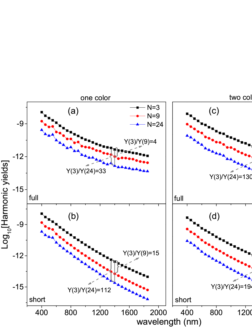
Figure 1: (Color online) Wavelength dependence of the HHG yield $Y(N,\lambda)$ for $N$-cycle one-color (a, b) and two-color (c, d) laser pulses. Results are obtained through full TDSE simulations (a, c) and the short-trajectory simulations (b, d). The ratio of $Y(N_{1})/Y(N_{2})$ at $\lambda=1400$ nm is also shown.

II Theoretical methods

To explore a wide range of laser wavelength, we first use a 2D H${}_{2}^{+}$ model, which has been widely used in theoretical studies Lein , to simulate the HHG.

The Hamiltonian of the model molecule studied here is H$(t)=\mathbf{p}^{2}/2+V(\mathbf{r})+\mathbf{r}\cdot\mathbf{E}(t)$ (in atomic units of $\hbar=e=m_{e}=1$). The potential used here has the form of $V(\mathbf{r})=-{Z}/{\sqrt{\xi+r_{1}^{2}}}-{Z}/{\sqrt{\xi+r_{2}^{2}}}$ with $r_{1,2}^{2}=({x\pm R/2\cos\theta})^{2}+(y\pm R/2\sin\theta)^{2}$. $R=2$ a.u. is the internuclear distance, $\xi=0.5$ is the smoothing parameter which is used to avoid the Coulomb singularity. $Z$ is the effective charge which is modulated in such a manner that the ground state of the model molecule has the ionization potential of $I_{p}=1.1$ a.u.. The latter is somewhat higher than that of the He atom. $\theta$ denotes the angle between the molecular axis and the laser polarization. Here, we have assumed that the laser polarization is along the $x$ axis and the molecular axis is located at the $xoy$ plane. We consider the perpendicular orientation with $\theta=90^{0}$ for which the molecule behaves similarly to an atom Chen . We work with a space grid size of $L_{x}\times L_{y}=1638.4\times 102.4$ a.u. for the $x$ and the $y$ axes. The electric field used here has the form of ${E}(t)=f(t){E_{0}}(\sin{\omega_{0}}t+\varepsilon\sin{2\omega_{0}}t)$ with $\varepsilon=0$ for one-color cases and $\varepsilon=0.5$ for two-color cases. $f(t)$ is the envelope function. To check the influence of the pulse duration on the HHG and simplify our discussions, we use a $3n$-cycle laser pulse which is switched on and off linearly over $n$ optical cycles with $n=1,3,8$. The whole pulse duration is $NT$ with $N=3n$ and $T=2\pi/\omega_{0}$.

We solve the time-dependent Schrödinger equation (TDSE) using the spectral method. In each time step, a mask function $\cos^{1/8}$ is used in the boundary to absorb the continuum wave packet. The coordinate position $x_{0}$ ($y_{0}$) from where the mask function becomes to work is $\pm L_{x}/8$ ($\pm L_{y}/8$). Alternatively, we can set $x_{0}=\pm E_{0}/w_{0}^{2}$ with $y_{0}=\pm L_{y}/8$ unchanged Yu . For our present cases, this treatment removes the contributions of the long trajectory and multiple returns to the HHG as the contribution of the short trajectory, which dominates experimental HHG Agostini , is not influenced basically. $E_{0}/w_{0}^{2}$ is the quiver amplitude of the classical electron in the laser field. Below, for differentiation from the full TDSE simulation with $x_{0}=\pm L_{x}/8$, we denote the simulation with setting $x_{0}=\pm E_{0}/w_{0}^{2}$ as the short-trajectory simulation.

Once the HHG power spectrum $S(\omega)$ for the harmonic $\omega$ is obtained from the TDSE dipole acceleration, we calculate the average HHG yield for a $N$-cycle laser pulse using $Y(N,\lambda)\propto\frac{1}{N(\Omega_{2}-\Omega_{1})}\int^{\Omega_{2}}_{\Omega_{1}}S(\omega)d\omega$. Here, $\Omega_{1}=I_{p}$ and $\Omega_{2}$ is the cutoff energy of the spectrum. $\lambda$ is the laser wavelength. For the pulse shape used here, $Y(N,\lambda)$ can be used to compare the HHG conversion efficiency at different pulse durations directly Gkortsas .

In the following, our discussions will be performed for a moderate laser intensity of $I=5\times 10^{14}$W/cm² at which the ionization yield of the model molecule is low.

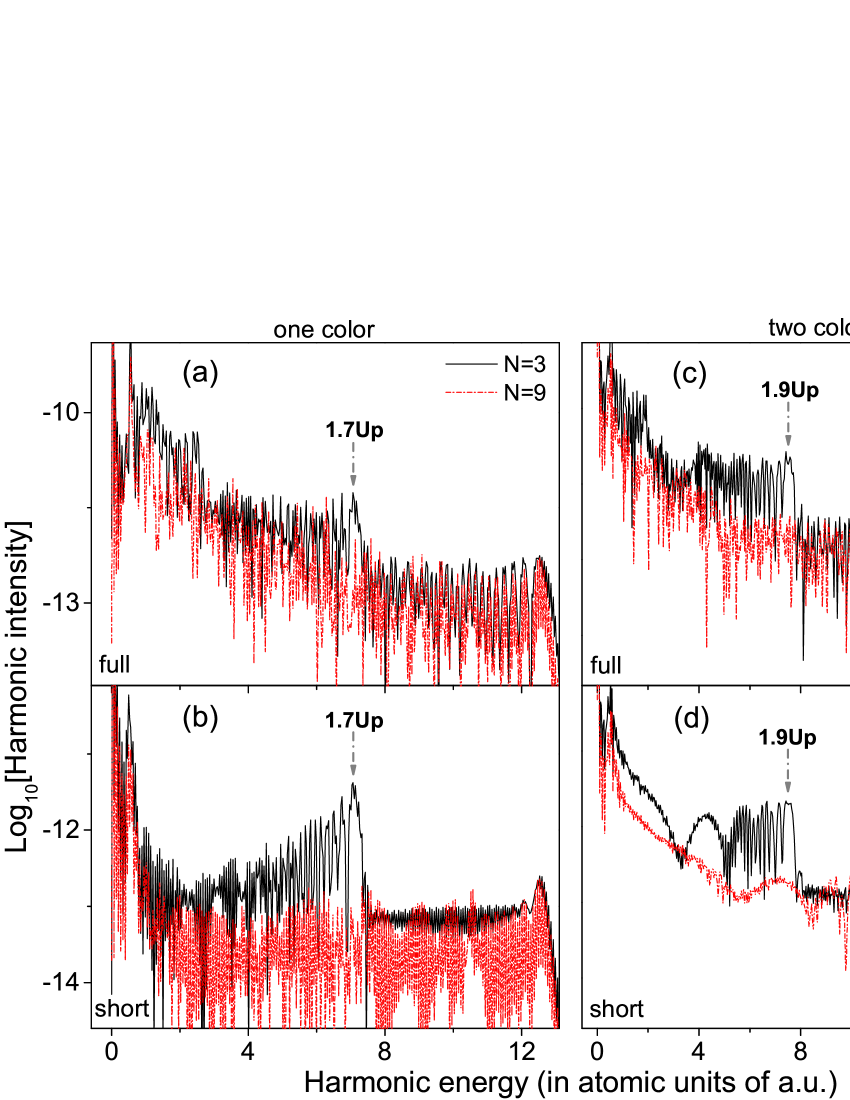
Figure 2: (Color online) HHG spectra for $N$-cycle one-color (a, b) and two-color (c, d) laser pulses at $\lambda=1400$ nm. Results are obtained through full TDSE simulations (a, c) and the short-trajectory simulations (b, d), and divided by the cycle number $N$.

III Enhanced HHG yield

In Fig. 1(a), we plot the wavelength dependence of the average HHG yield in a one-color field for different pulse durations. The contrast of the curves is remarkable. One can observe that the average HHG yield is the highest for the 3-cycle pulse at different wavelengthes. This yield decreases as the cycle number $N$ increases. At long wavelengthes such as $\lambda=1400$ nm, the yield of the 3-cycle pulse is several times higher than the 9-cycle result, and one order of magnitude higher than that of the 24-cycle pulse. Note, in this case, the whole HHG yield of $NY(N,\lambda)$ for $N=3$ is also several times higher than that for $N=24$. The contrast of the HHG yields at different pulse durations becomes more remarkable as the short-trajectory simulations are performed. As shown in Fig. 1(b), as the contributions of the long trajectory and multiple returns are excluded, the short-trajectory HHG yield for $N=3$ is one order of magnitude higher than $N=9$, and two orders of magnitude higher than $N=24$. For a two-color laser field, however, this remarkable difference occurs even for the full TDSE simulations, as shown in Fig. 1(c). Here, the ratio of $Y(3,\lambda)$ vs $Y(24,\lambda)$ with $\lambda=1400$ nm arrives at $130$, implying a significant increase of the HHG efficiency in a short two-color laser pulse. This significant increase of the efficiency is further amplified as the short-trajectory contributions are considered, as shown in Fig. 1(d). Since the short-trajectory simulations are closely associated with the classical motion of the electron, these results in Figs. 1(b) and 1(d) imply that the potential mechanism which increases the HHG yields at short pulses, is related to the classical aspect of the electron. Next, we explore the mechanism in detail.

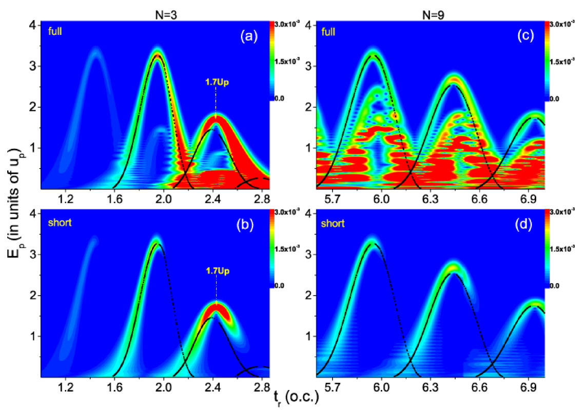
Figure 3: (Color online) Rescattering time and energy distributions (the color coding) for 3-cycle (a, b) and 9-cycle (c, d) one-color laser pulses at $\lambda=1400$ nm. Results are obtained through full TDSE simulations (a, c) and the short-trajectory simulations (b, d). In each panel, the black-square curve shows the electron trajectory for the first return, obtained from the quantum orbit model.

Figure 2 plots the HHG spectra of 3-cycle vs 9-cycle pulses for the typical wavelength of $\lambda=1400$ nm. For comparison, these spectra are divided by the cycle number $N$. For the one-color case in the left column of Fig. 2, one can observe from Fig. 2(a) of full simulations: i) the spectrum with $N=3$ (the solid-black curve) is higher than that of $N=9$ (the dashed-red curve), especially for the low-energy part. ii) In both cases, the HHG yield decreases as the harmonic energy increases. iii) The spectrum of $N=3$ shows three plateaus with the cutoff positions of $\omega=2.5$ a.u., $7.1$ a.u. and $12.5$ a.u. respectively. Around the second cutoff $\omega=7.1$ a.u. (corresponding to the electron kinetic energy of $E_{p}=\omega-I_{p}=1.7U_{p}$), a robust peak can be observed. As the short-trajectory simulation is executed, the robust peak of $N=3$ survives our treatments and the spectrum of $N=9$ becomes flat, resulting in a remarkable contrast of these two spectra with different $N$, as shown in Fig. 2(b).

For the two-color case, the contrast of the two spectra at different pulse durations is more remarkable, even for the full TDSE results, as shown in the right column of Fig. 2. In this case, the spectrum of $N=3$ in Fig. 2(c) of full simulations shows four plateaus with the cutoff positions of $\omega=1.9$ a.u., $7.6$ a.u., $11.3$ a.u. and $17.1$ a.u., respectively. Around the second plateau which also has a robust peak at $\omega=7.6$ a.u. (corresponding to $E_{p}=1.9U_{p}$), the spectrum of $N=3$ is one order of magnitude higher than that of $N=9$. The latter, by comparison, shows two striking plateaus corresponding to the third and the fourth plateaus of $N=3$. As we perform the short-trajectory simulations, the intensity of the second plateau does not decrease basically, as shown in Fig. 2(d). The origin of the plateaus can be well understood through the wavelet analysis of the TDSE dipole acceleration combined with the quantum orbit (QO) theory Lewenstein ; Salieres , as to be discussed below. These comparisons in Fig. 2 explain the remarkable difference for the HHG yields at different pulse durations discussed in Fig. 1. From the comparisons, one can also conclude that the high HHG efficiency of short pulses is closely related to the robust HHG peaks of $1.7U_{p}$ and $1.9U_{p}$ indicated in Fig. 2, which are less influenced by our different absorbing procedures in TDSE simulations. This conclusion can be further checked through the time-frequency analysis.

IV Classical effects

As a case, in Fig. 3, we show wavelet-analysis Tong results (the color coding) for the corresponding spectra in Figs. 2(a) and 2(b). For comparison, here, we also show the electron trajectory of the first return with the excursion time of the electron shorter than a laser cycle (the black-square curve), predicted from the QO model. For $N=3$, from Fig. 3(a) of the full TDSE results, one can observe that i) the distributions match the theory predictions basically; ii) the distributions imply three HHG cutoffs. The first one with $E_{p}=0.5U_{p}$ around the return time $t_{r}=2.4T$ has the largest amplitude. The second one with $E_{p}=1.7U_{p}$ also appears around $t_{r}=2.4T$ and has a comparable amplitude with the first one, as indicated by the dashed arrow. The third one with $E_{p}=3.2U_{p}$ near to $t_{r}=2T$ has the smallest amplitude. The first one can be identified as arising from multiple returns, and the second and the third ones come from the first return. For short-trajectory simulations in Fig. 3(b), the first one disappears, as the second and the third ones keep their amplitudes with the prevailing role of the second one. Note, the contributions of the long trajectory around the minus-chirp part of the black-square curve also disappear basically due to the absorbing procedure used here. For $N=9$, the situation is different. The full TDSE results in Fig. 3(c) show large amplitudes around the electron trajectories of multiple returns (these trajectories are not shown here), in agreement with the results in Ref. Tate . In Fig. 3(d) of short-orbital simulations, the contributions of multiple returns disappear. The survived distributions, however, show smaller amplitudes than that around $E_{p}=1.7U_{p}$ in Fig. 3(b). To understand the large amplitude located at $E_{p}=1.7U_{p}$ in Fig. 3(b), in Fig. 4, we further compare the maximal displacement $x_{m}$ Yu , which the electron can travel as it ionizes at the time $t_{i}$ and returns at $t_{r}$ for $N=3$ vs $N=9$.

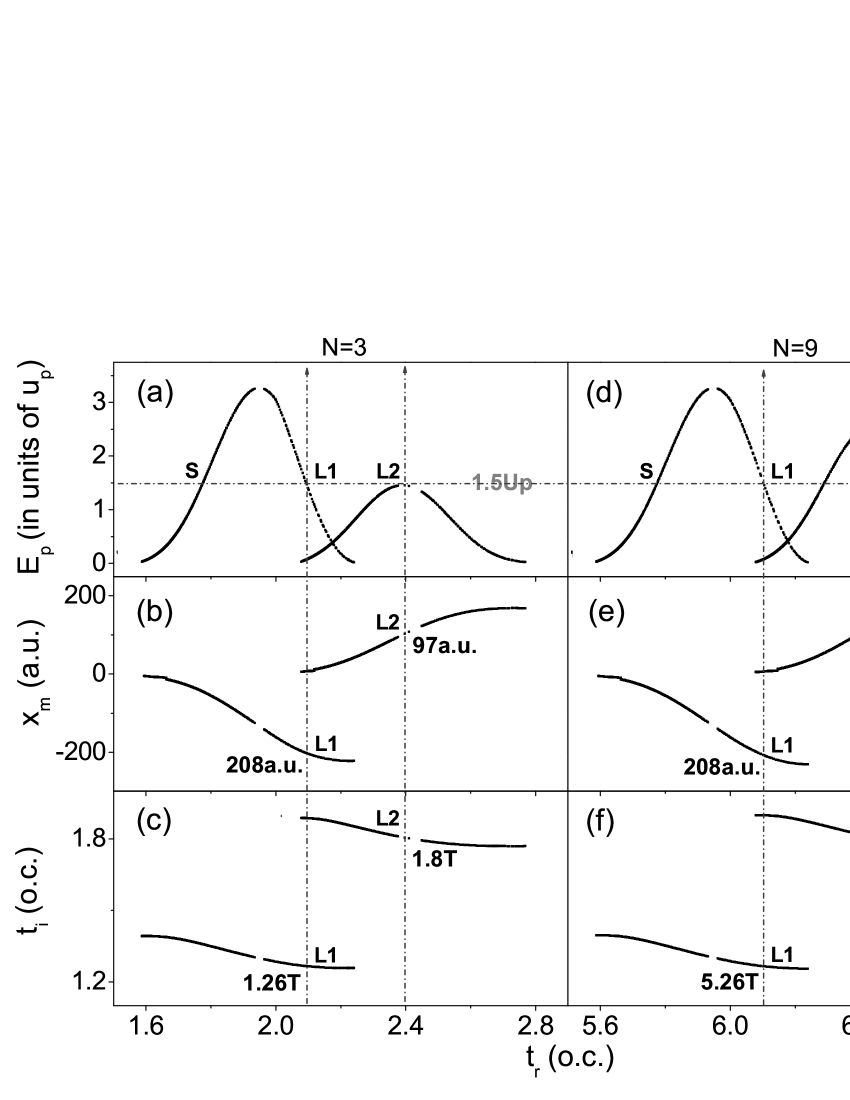
Figure 4: The kinetic energy $E_{p}$, the maximal displacement $x_{m}$ and the ionization time $t_{i}$ of the rescattering electron as functions of the return time $t_{r}$ for 3-cycle (the left column) and 9-cycle (the right column) one-color laser pulses at $\lambda=1400$ nm, obtained using the quantum orbit model. Only the first return with the excursion time $\tau=t_{r}-t_{i}<T$ is shown. The horizontal arrow indicates the orbits with $E_{p}=1.5U_{p}$ for short (S) and long (L1 and L2) trajectories. The vertical arrows indicate the corresponding $x_{m}$ and $t_{i}$ of theses two long trajectories. The relevant values of $x_{m}$ and $t_{i}$ are as shown.

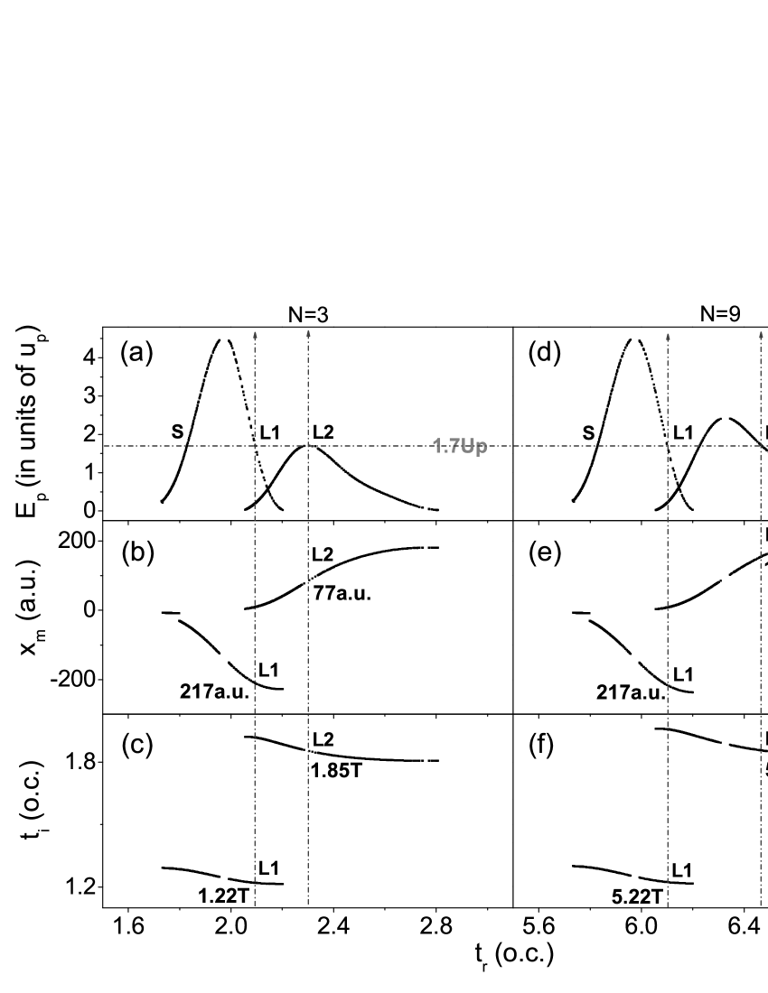
Figure 5: Same as Fig. 4, but for two-color laser pulses.

To obtain the maximal displacement $x_{m}$, we first calculate the complex ionization time $t^{q}_{i}$ and the return time $t^{q}_{r}$ (the real parts of the complex times are considered the physical ionization time $t_{i}$ and the return time $t_{r}$) by the QO model. Then we evaluate the maximal displacement using Becker2 $x_{m}\equiv x_{m}(t)=(E_{0}/\omega_{0}^{2})Re[\sin\omega_{0}t-\sin\omega_{0}t_{i}^{q}+p_{st}(\omega_{0}^{2}/E_{0})(t-t_{i}^{q})]$ with $v(t)=Re[p_{st}+E_{0}/\omega_{0}\cos(\omega_{0}t)]=0$ and $Re(t_{i}^{q})<t<Re(t_{r}^{q})$. $v(t)$ is the electron velocity, and $p_{st}=(E_{0}/\omega_{0})[\sin\omega_{0}t_{i}^{q}-\sin\omega_{0}t_{r}^{q}]/[\omega_{0}(t_{r}^{q}-t_{i}^{q})]$ is the saddle-point momentum. We mention the maximal displacement obtained here agrees well with that obtained using the classical procedure introduced in Ref. Yu .

Our comparisons are performed for two typical long trajectories (denoted using $L1$ and $L2$ in Fig. 4) with the same return energy $E_{p}=1.5U_{p}$, near to $E_{p}=1.7U_{p}$ of the large amplitude in Fig. 3(b). Both these two trajectories have the ionization times $t_{i}$ located in the flat-top part of the pulse and near to the peak of the field, as shown in Figs. 4(c) and 4(f), and are expected to contribute importantly to the HHG. The return times of the two trajectories are different. As the $L1$ trajectory returns near to the flat-top part of the pulse, the $L2$ trajectory returns in the falling part of the pulse (the laser pulse becomes to fall at 2T for $N=3$ and 6T for $N=9$). For the 3-cycle case in Fig. 4(b), the displacement $x_{m}$ for the $L2$ trajectory is 97 a.u.. It is 208 a.u. for $L1$, two times larger than the $L2$ one. Considering the spread of the wave packet is proportional to the electron displacement, these above results imply the $L2$ trajectory has a amplitude several times larger than the $L1$ one, in agreement with the wavelet-analysis result in Fig. 3(b). For the 9-cycle case in Fig. 4(e), the situation is different. The $L2$ trajectory has the maximal displacement of $x_{m}=185$ a.u. which is near to 208 a.u. of the $L1$ one. As a result, the wave packet spreading is comparable for the two trajectories in the 9-cycle case, resulting in similar amplitudes for them, as seen in Fig. 3(d). We mention that short trajectories have the smaller displacements $x_{m}$ than the corresponding long ones. However, they usually ionize at a time farther away from the peak of the field and therefore have smaller amplitudes than the long ones (this can also be seen from the wavelet-analysis results in Fig. 3). For the reason, we don’t discuss them here.

In combination with the distributions in Fig. 3(b) vs Fig. 3(d), the contrast of the maximal displacements $x_{m}$ for the $L2$ trajectory in Fig. 4(b) vs Fig. 4(e) suggests that the higher HHG efficiency for the short pulse of $N=3$, observed in Fig. 1(b), is closely related to the shorter excursion distance of the electron in the fast falling part of the short pulse. This classical effect which increases the HHG efficiency becomes more remarkable in the two-color case, as shown in Fig. 5. Here, our analyses are also performed for two typical long trajectories of $L1$ and $L2$. The ionization times of the two long trajectories both are located at the flat-top part of the pulse and are near to the peaks of the two-color field, as shown in Figs. 5(c) and 5(f). In addition, the electric-field amplitudes at the two ionization times of $L1$ and $L2$ in the two-color case are nearer to each other than in the one-color one. For the short-pulse case of $N=3$, one can observe from Fig. 5(b) that the maximal displacement of the $L2$ trajectory is $x_{m}=77$ a.u., as the $L1$ trajectory shows a maximal displacement of $x_{m}=217$ a.u., almost three times larger than the $L2$ one. For the long-pulse case of $N=9$, they are 154 a.u. and 217 a.u., respectively, as shown in Fig. 5(e). The shorter excursion distance of the $L2$ trajectory in Fig. 5(b) of $N=3$, suggests that this trajectory contributes significantly to the HHG in the short-pulse case. It is corresponding to the cutoff of the second plateau with high intensity in Figs. 2(c) and 2(d). We mention that the TDSE cutoff position of the second plateau in Fig. 2(c) is $1.9U_{p}$ for the 3-cycle case, somewhat higher than the model prediction of $1.7U_{p}$ in Fig. 5(a). This is also the one-color case of $1.7U_{p}$ in Fig. 2(a) versus $1.5U_{p}$ in Fig. 4(a). This difference can partly arise from the nonadiabatic effect in ultrashort pulses. In comparison with $x_{m}=97$ a.u. with $E_{p}=1.5U_{p}$ in Fig. 4(b), this shorter excursion distance $x_{m}=77$ a.u. of the $L2$ trajectory with the higher return energy $E_{p}=1.7U_{p}$ in Fig. 5(b) also suggests the HHG efficiency is higher in the two-color case than in the one-color case, in agreement with our analyses in Fig. 1.

V Extended considerations

V.1 Three-dimensional simulations

To check our results, we have also performed 3D simulations for H${}_{2}^{+}$ with the soft-core potential of $V(\mathbf{r})=-{Z}/{\sqrt{\xi+r_{1}^{2}}}-{Z}/{\sqrt{\xi+r_{2}^{2}}}$ and $r_{1,2}^{2}=({x\pm R/2\cos\theta})^{2}+(y\pm R/2\sin\theta)^{2}+z^{2}$. The Definitions of the parameters $Z$, $\xi$, $R$ and $\theta$ are the same as in our 2D cases. The 3D calculations are very time-memory consuming. Here, we work with a grid size of $L_{x}\times L_{y}\times L_{z}=819.2\times 51.2\times 51.2$ a.u. for the $x$, $y$ and $z$ axes, respectively. Our calculations are performed for $I=5\times 10^{14}$W/cm² and $\lambda=1400$ nm corresponding to the laser parameters used in Fig. 2. Similar absorbing procedures as in 2D cases are also used in performing full TDSE simulations and short-trajectory simulations. The results are presented in Fig. 6.

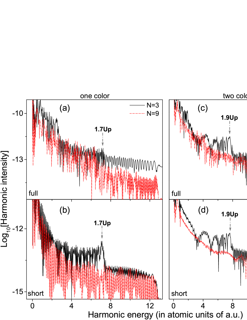
Figure 6: (Color online) Same as Fig. 2, but obtained with 3D simulations.

One can observe from Fig. 6 that the 3D results are similar to the 2D ones in Fig. 2. First, the spectra of $N=3$ show a robust peak which appears around $E_{p}=\omega-I_{p}=1.7U_{p}$ for one-color cases in the left column of Fig. 6 and around $E_{p}=1.9U_{p}$ for two-color cases in the right column of Fig. 6. Secondly, this robust peak is more remarkable in short-trajectory simulations than in full simulations and in two-color cases than in one-color cases. As discussed in Fig. 2, this robust peak arises from the classical effect, which increases the HHG efficiency importantly in short pulses. The 3D results in Fig. 6 also show that this HHG efficiency is strikingly higher in the short pulse than in the lone one. All of the characteristics are in agreement with our 2D results in Fig. 2.

One of the main differences between 2D and 3D cases is that the diffusion effect relating the wave packet spreading is stronger in 3D cases than in 2D cases. This stronger diffusion effect can induce a larger phase difference between the harmonics emitted in different laser cycles, especially for harmonics arising from the long trajectory and multiple returns with longer excursion times in the laser field. The interference of the harmonics emitted in different laser cycles will decrease the intensity of the HHG spectra and this decrease is more remarkable for long pluses with more cycles. This can be the reason that the spectrum of $N=9$ in Fig. 6(a) of full TDSE simulations shows a smaller amplitude in comparison with that of $N=3$ in the high-energy region with $\omega>7$ a.u.. Note that in Fig. 6(b) of short-trajectory simulations, these two spectra of $N=3$ and $N=9$ are comparable for the high-energy region of $\omega>7$ a.u., as the contributions of the long trajectory and multiple returns are excluded.

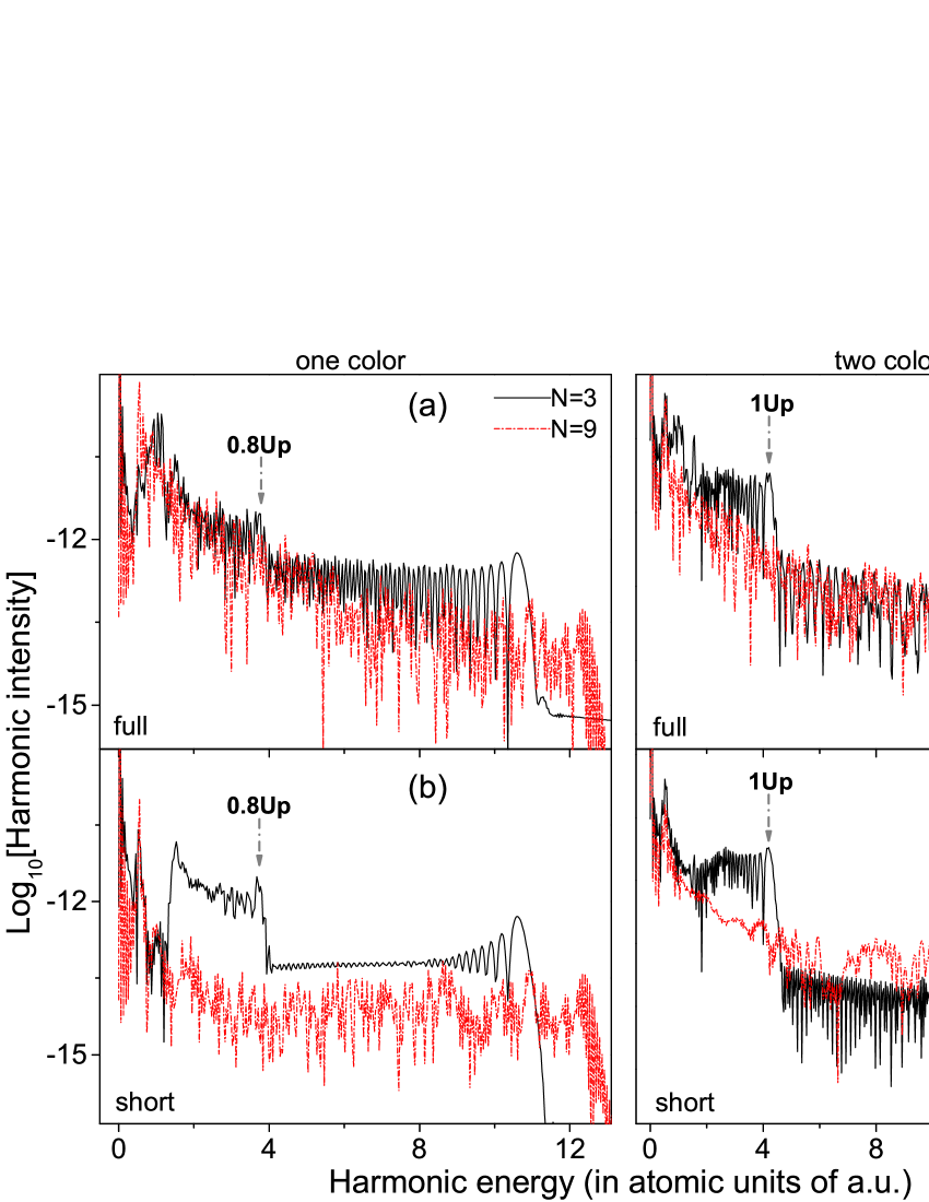
Figure 7: (Color online) Same as Fig. 2, but obtained for a sin-square-envelope laser pulse.

V.2 Sin-square-envelope pulses

To check our results, a sin-square-envelope pulse is also used in our calculations and relevant results are presented in Fig. 7. The results in Fig. 7 are also similar to those in Fig. 2, with showing a robust peak in the spectra of $N=3$. Here, the position of the peak is around $E_{p}=0.8U_{p}$ for one-color cases and $E_{p}=U_{p}$ for two-color cases, somewhat lower than those in Fig. 2. In addition, the maximal cutoff position of the spectrum of $N=3$ is also somewhat lower than that of $N=9$. However, in comparison with the results in Fig. 2, the results for $N=3$ presented here show higher inversion efficiency. For example, in Fig. 7(b), the spectrum of $N=3$ is higher than that of $N=9$ in the whole energy region, different from the results in Fig. 2(b). In addition, the curve of $N=3$ in Fig. 7(d) also shows a cutoff located at $\omega=13.5$ a.u.. Around the cutoff, the spectrum of $N=3$ is two orders of magnitude higher than that of $N=9$. All of the characteristics can be understood by virtue of the analyses of the quantum orbit and the maximal displacement of the rescattering electron.

V.3 High laser intensities

As the laser intensity increases and is near to the saturation intensity, the situation is somewhat different. As shown in Fig. 8(a), for the case of $I=1.2\times 10^{15}$W/cm² and $\lambda=1400$ nm, the HHG spectrum of $N=3$ is higher than that of $N=9$ in the whole energy region, even the average over the cycle number $N$ is not performed here. This can be understood from the ground-state deletion. For the long pulse of $N=9$, the ionization is stronger than that of $N=3$, resulting in a significant deletion of the ground state and accordingly a remarkable decrease of the HHG yield. However, in this case, the classical effect can still be read from the spectrum, which manifests itself as a harmonic peak around $E_{p}=1.75U_{p}$, as indicated by the dashed-dotted arrow. This peak is more remarkable in short-trajectory simulations, as shown in Fig. 8(b). In addition, the cutoff position in the spectrum of $N=3$ in Fig. 8(a) seems somewhat larger than that of $N=9$. This phenomenon is clearer for the case of $I=1\times 10^{15}$W/cm² and $\lambda=1600$ nm, as shown in Fig. 8(c). We mention that for the case in Fig. 8(c), the ionization is somewhat weaker than that in Fig. 8(a). Accordingly, the spectra of $N=3$ and $N=9$ are comparable here. In addition, a harmonic peak around $\omega=1.78U_{p}$ can also be observed in the spectrum of $N=3$ in Fig. 8(c). This peak is more striking in Fig. 8(d) of short-trajectory simulations. These results show that the classical effect, mainly discussed in the paper, is general in a wide laser-parameter region.

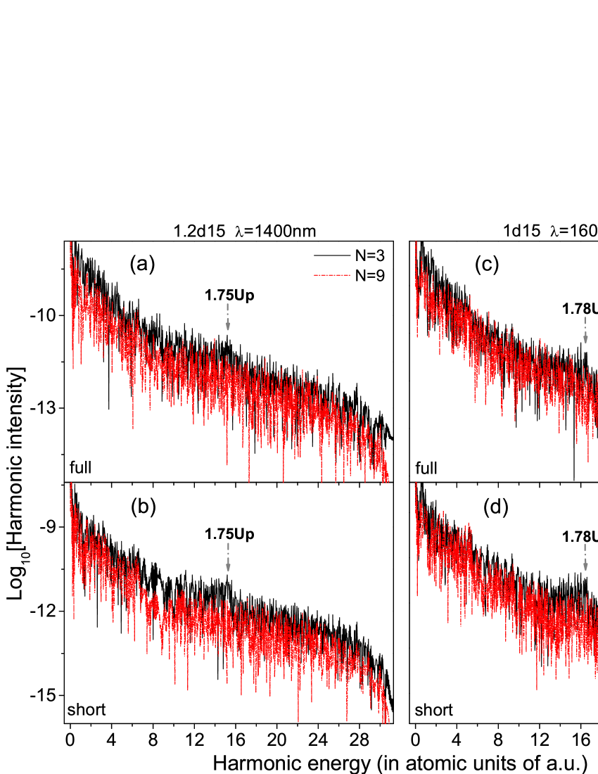
Figure 8: (Color online) HHG spectra for $N$-cycle one-color laser pulses at $I=1.2\times 10^{15}$W/cm² and $\lambda=1400$ nm (a, b) and $I=1\times 10^{15}$W/cm² and $\lambda=1600$ nm (c, d). Results are obtained through full TDSE simulations (a, c) and the short-trajectory simulations (b, d) in 2D cases.

VI Conclusions

In summary, we have shown that the HHG efficiency in an ultrashort laser pulse is influenced significantly by a classical effect. The latter is closely associated with the shorter excursion distance of the rescattering electron as it ionizes near the peak of the short laser pulse and returns in the fast falling part of the pulse. This shorter excursion distance suppresses the spread of the wave packet and increases the efficiency of the HHG. With the shorter excursion distance and accordingly the shorter excursion time, the emitted harmonics relating to the classical effect can be easier to survive the macroscopic propagation in the medium and easier to modulate in experiments. We expect that this effect also has an important influence on the rescattering induced other strong-field phenomena such as high-order above threshold ionization and nonsequential double ionization.

References

- (1) Philippe Antoine, Anne L’ Huillier, and Maciej Lewenstein, Phys. Rev. Lett. 77, 1234 (1996).
- (2) M. Drescher, M. Hentschel, R. Kienberger, G. Tempea, C. Spielmann, G. A. Reider, P. B. Corkum, F. Krausz, Science 291, 1923 (2001).
- (3) P. B. Corkum and F. Krausz, Nat. Phys. 3, 381 (2007).
- (4) Zenghu Chang, Andy Rundquist, Haiwen Wang, Margaret M. Murnane, and Henry C. Kapteyn, Phys. Rev. Lett. 79, 2967 (1997).
- (5) Y. Mairesse, A. de Bohan, L. J. Frasinski, H. Merdji, L. C. Dinu, P. Monchicourt, P. Breger, M. Kovačev, R. Taïeb, B. Carré, H. G. Muller, P. Agostini, P. Salières, Science 302, 1540 (2003).
- (6) J. Itatani, J. Levesque, D. Zeidler, Hiromichi Niikura, H. Pepin, J. C. Kieffer, P. B. Corkum, and D. M. Villeneuve, Nature (Londun) 432, 867 (2004).
- (7) P. B. Corkum, Phys. Rev. Lett. 71, 1994 (1993).
- (8) I. P.Christov, J. Zhou, J. Peatross, A. Rundquist, M. M. Murnane, and H. C. Kapteyn, Phys. Rev. Lett. 77, 1743 (1996).
- (9) T. Ditmire, K. Kulander, J. Crane, H. Nguyen, and M. Perry, J. Opt. Soc. Am. B 13, 406 (1996).
- (10) J. Tate, T. Auguste, H. G. Muller, P. Salières, P. Agostini, and L. F. DiMauro, Phys. Rev. Lett. 98, 013901 (2007).
- (11) A. D. Shiner, C. Trallero-Herrero, N. Kajumba, H.-C. Bandulet, D. Comtois, F. Légaré, M. Giguère, J-C. Kieffer, P. B. Corkum, and D. M. Villeneuve, Phys. Rev. Lett. 103, 073902 (2009).
- (12) Anh-Thu Le, Hui Wei, Cheng Jin, Vu Ngoc Tuoc, Toru Morishita, and C. D. Lin, Phys. Rev. Lett. 113, 033001 (2014).
- (13) Vasileios-Marios Gkortsas, Siddharth Bhardwaj, Edilson L Falcão-Filho, Kyung-Han Hong, Ariel Gordon and Franz X Kärtner, J. Phys. B 44, 045601 (2011).
- (14) I Jong Kim, Chul Min Kim, Hyung Taek Kim, Gae Hwang Lee, Yong Soo Lee, Ju Yun Park, David Jaeyun Cho, and Chang Hee Nam, Phys. Rev. Lett. 94, 243901 (2005).
- (15) V. Yakovlev, M. Ivanov, and F. Krausz, Opt. Express 15, 15351 (2007).
- (16) Pengfei Lan, Eiji J. Takahashi, and Katsumi Midorikawa, Phys. Rev. A 81, 061802(R) (2010).
- (17) Ivan P. Christov, Margaret M. Murnane, and Henry C. Kapteyn, Phys. Rev. Lett. 78, 1251 (1997).
- (18) M. Schnürer, Ch. Spielmann, P. Wobrauschek, C. Streli, N. H. Burnett, C. Kan, K. Ferencz, R. Koppitsch, Z. Cheng, T. Brabec, and F. Krausz, Phys. Rev. Lett. 80, 3236 (1998).
- (19) Armelle de Bohan, Philippe Antoine, Dejan B. Milošević, and Bernard Piraux, Phys. Rev. Lett. 81, 1837 (1998).
- (20) P. Villoresi, P. Ceccherini, L. Poletto, G. Tondello, C. Altucci, R. Bruzzese, C. de Lisio, M. Nisoli, S. Stagira, G. Cerullo, S. De Silvestri, and O. Svelto, Phys. Rev. Lett. 85, 2494 (2000).
- (21) T. Brabec and F. Krausz, Rev. Mod. Phys. 72, 545 (2000).
- (22) J. Mauritsson, P. Johnsson, E. Gustafsson, A. L Huillier, K. J. Schafer, and M. B. Gaarde, Phys. Rev. Lett. 97, 013001 (2006).
- (23) N. Dudovich, O. Smirnova, J. Levesque, Y. Mairesse, M. Yu. Ivanov, D. M. Villeneuve, and P. B. Corkum, Nat. Phys. 2, 781 (2006).
- (24) Zhinan Zeng, Ya Cheng, Xiaohong Song, Ruxin Li, and Zhizhan Xu, Phys. Rev. Lett. 98, 203901 (2007).
- (25) Hiroki Mashiko, Steve Gilbertson, Chengquan Li, Sabih D. Khan, Mahendra M. Shakya, Eric Moon, and Zenghu Chang, Phys. Rev. Lett. 100, 103906 (2008).
- (26) F. Krausz and M. Ivanov, Rev. Mod. Phys. 81, 163 (2009).
- (27) M. Lein, N. Hay, R. Velotta, J. P. Marangos, and P. L. Knight, Phys. Rev. Lett. 88, 183903 (2002).
- (28) Y. Chen, Y. Li, S. Yang, and J. Liu, Phys. Rev. A 77, 031402(R) (2008).
- (29) S. J. Yu, B. Zhang, Y. P. Li, S. P. Yang, and Y. J. Chen, Phys. Rev. A 90, 053844 (2014).
- (30) P. Agostini and L. F. DiMauro, Rep. Prog. Phys. 67, 813 (2004).
- (31) M. Lewenstein, Ph. Balcou, M. Yu. Ivanov, A. L’Huillier, and P. B. Corkum, Phys. Rev. A 49, 2117 (1994).
- (32) P. Salieres, B. Carre, L. Le Deroff, F. Grasbon, G. G. Paulus, H. Walther, R. Kopold, W. Becker, D. B. Milosevic, A. Sanpera, and M. Lewenstein, Science 292, 902 (2001).
- (33) X. M. Tong and S.-I. Chu, Phys. Rev. A 61, 021802(R) (2000).
- (34) D. B. Milosěvić and W. Becker, Phys. Rev. A 66, 063417 (2002).
- (35) chenyjhb@gmail.com