Bayesian ensemble refinement by replica simulations and reweighting

Abstract

We describe different Bayesian ensemble refinement methods, examine their interrelation, and discuss their practical application. With ensemble refinement, the properties of dynamic and partially disordered (bio)molecular structures can be characterized by integrating a wide range of experimental data, including measurements of ensemble-averaged observables. We start from a Bayesian formulation in which the posterior is a functional that ranks different configuration space distributions. By maximizing this posterior, we derive an optimal Bayesian ensemble distribution. For discrete configurations, this optimal distribution is identical to that obtained by the maximum entropy “ensemble refinement of SAXS” (EROS) formulation. Bayesian replica ensemble refinement enhances the sampling of relevant configurations by imposing restraints on averages of observables in coupled replica molecular dynamics simulations. We show that the strength of the restraint should scale linearly with the number of replicas to ensure convergence to the optimal Bayesian result in the limit of infinitely many replicas. In the “Bayesian inference of ensembles” (BioEn) method, we combine the replica and EROS approaches to accelerate the convergence. An adaptive algorithm can be used to sample directly from the optimal ensemble, without replicas. We discuss the incorporation of single-molecule measurements and dynamic observables such as relaxation parameters. The theoretical analysis of different Bayesian ensemble refinement approaches provides a basis for practical applications and a starting point for further investigations.

I Introduction

The problem of ensemble refinement Boomsma, Ferkinghoff-Borg, and Lindorff-Larsen (2014) becomes increasingly important as structural biology enters a new era in which dynamic and partially disordered biomolecular structures come into focus.Sali et al. (2015); Boura et al. (2011); Ward, Sali, and Wilson (2013) Such systems play central roles in biology, both in functional cellular processes ranging from signal transduction to the formation of large cellular structures, and in disease, including neurodegenerative diseases such as Parkinson’s and Alzheimer’s. A broad range of methods have been developed to refine models of (bio)molecular structures against experimental data from X-ray crystallography, nuclear magnetic resonance (NMR) spectroscopy, electron microscopy (EM), solution X-ray or neutron scattering (SAXS, SANS), and other methods. By and large, these refinement methods operate under the assumption that a single or a few well ordered structures should account for all the measurements. However, refinement of a single (or possibly a few) copies is not appropriate in systems with significant disorder. For unfolded Camilloni and Vendruscolo (2014) or intrinsically disordered proteins (IDP),Fisher, Huang, and Stultz (2010); Fisher and Stultz (2011); Sanchez-Martinez and Crehuet (2014) such as the $\alpha$-synuclein peptide involved in Parkinson’s disease,Dedmon et al. (2005); Mantsyzov et al. (2014, 2015) we expect that a very broad range of structures is present in solution. None of these structures may individually satisfy all measurements, and even if one did, it may be highly atypical. Instead, most observables accessible to experiment report on averages over the entire ensemble of structures, and as such only the appropriate average over a model ensemble should match the experiment.

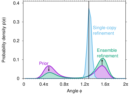
Figure 1: Illustrative comparison of refined probability densities $p(\phi)$ of a dihedral angle $\phi$ from single-copy refinement [blue; Eqs. (2-4); every member of the ensemble is expected to satisfy the measurement individually] and ensemble refinement [green; Eq. (II.2); the ensemble average is expected to satisfy the measurement]. The prior or reference distribution (magenta) used in the refinements is bimodal, i.e., with two dominant rotamer states. As indicated by the vertical black line, the observable is $y(\phi)\equiv\phi=1.28\pi$ for single-copy refinement and $Y\equiv\overline{\phi}=1.28\pi$ for ensemble refinement, with “experimental” error $\sigma=0.04\pi$ in both cases, and $\theta=1$. Arrows indicate the changes in the relative weights of the two rotamers in the optimal Bayesian ensemble refined distribution.

Ensemble refinement is a challenging inverse problem in which one aims to characterize the high-dimensional configuration space of a molecular system on the basis of limited experimental information. It is therefore essential that ensemble refinement methods can properly integrate data from a broad range of experiments Ward, Sali, and Wilson (2013); Schröder (2015); Sali et al. (2015) that may report on molecular size and shape (e.g., from SAXS, SANS, or hydrodynamic measurements Rozycki, Kim, and Hummer (2011); Boura et al. (2011); Francis et al. (2011)), the proximity (e.g., from cross-links) or distance between atoms and residues [e.g., from fluorescence resonant energy transfer (FRET), NMR,Scheek et al. (1991); Lange et al. (2008); Olsson et al. (2014) including nuclear Overhauser effects (NOE), or double electron-electron resonance (DEER) measurements Boura et al. (2011, 2012)], the local chemical environment and structure (e.g., from NMR chemical shifts Francis et al. (2011) and J-couplings Mantsyzov et al. (2014, 2015) or X-ray absorption spectroscopy), all the way to measures of the global structure (e.g., from X-ray crystal diffraction or electron microscopy Cossio and Hummer (2013); Ward, Sali, and Wilson (2013); Schröder (2015)). Taking into account the uncertainties of the different experiments Schneidman-Duhovny, Pellarin, and Sali (2014) is critical for the construction of a properly weighted configurational ensemble.

Inverse problems are typically ill-conditioned, i.e., sensitive to input parameter variations, and underdetermined. Such problems with high sensitivity and low data-to-parameter ratios are usually tackled through regularization, for instance by assuming near-uniform and smooth solutions. Bayesian statistics offers a particularly elegant route for the inference of probabilistic models from data (see, e.g., Ref. MacKay, 2003 for a general overview and Ref. Rieping, Habeck, and Nilges, 2005 for a pioneering application to biomolecular studies). In effect, the assumed prior distributions of the model parameters serve as regularizing factors,

$$p(\textrm{model}|\textrm{data})\propto p(\textrm{data}|\textrm{model})p_{0}(\textrm{model}),$$ (1)

written as a proportionality without the normalizing factor. $p(\textrm{model}|\textrm{data})$ is the posterior distribution of the model, and $p_{0}(\textrm{model})$ is the prior that expresses our expectations on the model and its parameters in the absence of new data. $p(\textrm{data}|\textrm{model})$ is the conditional probability of observing the data given the model, which for given data is the likelihood of the model. Consequently, we will in the following refer to $p(\textrm{data}|\textrm{model})$ as the likelihood function. Importantly, in the absence of new data (or for non-informative data), one simply recovers the prior.

The importance of ensemble refinement is best illustrated by a simple example that anticipates some of the theoretical developments in this work. Figure 1 contrasts the stark differences in the results for single-copy and ensemble refinements of a simple model system with a prior or reference distribution with two dominant rotamers. In single-copy refinement, we determine how well each dihedral angle $\phi$ individually agrees with the observation $y^{(\mathrm{obs})}=\phi^{(\mathrm{obs})}=1.28\pi$. This posterior probability $p(\phi|\mathrm{data})\equiv p(\phi|y^{(\mathrm{obs})})$ is concentrated in a sharp peak around the target value. By contrast, in ensemble refinement we seek a probability density $p(\phi)$ that is consistent with the observed average $Y^{(\mathrm{obs})}\equiv\overline{\phi}$. This $p(\phi)\equiv p^{\mathrm{(opt})\!}(\phi)$ retains the character of the reference distribution that reflects the underlying physics, while redistributing some population from one rotamer to the other.

Here, we will describe both formal and practical approaches toward inferring ensemble distributions from diverse data. We will formulate the ensemble refinement problem first formally in a Bayesian framework in which the posterior is a functional that quantifies the relative probability of different ensemble probability densities $p(\mathbf{x})$ for configurations $\mathbf{x}$. Experimental uncertainties Schneidman-Duhovny, Pellarin, and Sali (2014) are taken into account from the outset, which allows us to combine data from a variety of measurements. We then study algorithms to realize Bayesian ensemble refinement in practice. First, we will describe a method with which existing ensembles can be reweighted to match experiment. By variational maximization of the Bayesian posterior functional over the ensemble probability densities $p(\mathbf{x})$, we will derive an optimal Bayesian ensemble density $p^{\mathrm{(opt})\!}(\mathbf{x})$, Eq. (II.2), for the continuous case and Eq. (II.2) for the discrete case. Applied to sub-ensembles drawn according to the prior, this reweighting method turns out to be equivalent to the maximum entropy refinement procedure in the ensemble refinement of SAXS (EROS) method Rozycki, Kim, and Hummer (2011) (which is different from the “ensemble refinement with orientational restraints” method with the same acronym Lange et al. (2008)). In the limit of infinite sample size, the reweighting method converges to the optimal Bayesian ensemble refinement. Then, we will describe a Bayesian replica ensemble refinement method to perform ensemble refinement on the fly by running molecular simulations of identical copies of the system with a bias on the averages calculated over these replicas. If the biasing potential is proportional to chi-squared (as twice the negative log-likelihood for Gaussian errors) scaled by the number of replicas $N$ [see Eq. (II.3)], one recovers the optimal Bayesian ensemble refinement [Eq. (II.2)] in the limit of an infinite number of replicas. At the other extreme, in the limit of a single replica, the common-property refinement [Eq. (12)] is recovered, in which every member of the ensemble is expected to satisfy the measurements individually, not just in the ensemble average. To speed up the convergence to the optimal Bayesian distribution with increasing number of replicas $N$, we show how EROS and replica refinement (as well as other ensemble-biased simulation methods) can be combined with the help of free-energy reweighting methods, resulting in the “Bayesian inference of ensembles” (BioEn) method. An adaptive algorithm designed to sample directly from the optimal ensemble distribution, without multiple replicas, is presented in an Appendix.

To illustrate the formal theory and the practical replica simulation approaches, we will introduce analytically or numerically tractable models of ensemble refinement. The solutions obtained for these models allow us to assess the mutual consistency of the methods, and to demonstrate the need for a size-consistent treatment in the Bayesian replica ensemble refinement with respect to the number of replicas. We also sketch how dynamic properties can be integrated in ensemble refinement, albeit approximately, and how the parameter expressing the confidence in the reference ensemble distribution can be chosen. We conclude by a summary of the main results and a discussion of possible applications, including the optimization of potential energy functions used for molecular simulations.

II Theory

II.1 Bayesian single-copy refinement in configuration space

Before venturing into ensemble refinement, we introduce notation and the general framework in the context of the more familiar single-copy refinement. Here one assumes that a single configuration can explain all measured data. Different configurations can then be ranked, in a probabilistic manner, by their respective abilities to do so.

In the following, we will use $\mathbf{x}$ to denote individual configurations. In a typical application to a molecular system, $\mathbf{x}$ could be the $3n$-dimensional vector $\mathbf{x}=\left\{\mathbf{r}_{1},\mathbf{r}_{2},\ldots,\mathbf{r}_{n}\right\}$ of the Cartesian coordinates $\mathbf{r}_{i}$ of the $n$ atoms. In single-copy refinement, we assume that one would ideally (i.e., without error) measure values $y_{i}(\mathbf{x})$ of observable $i$, with $i=1,2,\ldots,M$, for a given configuration $\mathbf{x}$. The actual values observed (measured) are $y_{i}^{(\mathrm{obs})}$. By contrast, in ensemble refinements described below, the measured values of the observables will instead depend on the distribution over the entire configuration space, not just on a single configuration $\mathbf{x}$.

Using a reference distribution $p_{0}(\mathbf{x})$ as a prior, in single-copy refinement we want to construct a posterior $p(\mathbf{x}|\mathrm{data})$ in configuration space that ranks configurations $\mathbf{x}$ by their consistency with both experimental measurements and prior. The prior $p_{0}(\mathbf{x})$ could for instance be the Boltzmann distribution for a simulation model described by a particular potential energy function $U(\mathbf{x})$, i.e., $p_{0}(\mathbf{x})=\exp[-\beta U(\mathbf{x})]/\int d\mathbf{x}^{\prime}\exp[-\beta U(\mathbf{x}^{\prime})]$ at reciprocal temperature $\beta=1/k_{B}T$ with $k_{B}$ the Boltzmann constant and $T$ the absolute temperature, or a statistical distribution of conformers of the Protein Data Bank.Mantsyzov et al. (2014, 2015) The normalized posterior distribution according to Eq. (1) is then

$$p(\mathbf{x}|\{y_{i}^{(\mathrm{obs})}\})=\frac{p_{0}(\mathbf{x})p(\{y_{i}^{(\mathrm{obs})}\}|\mathbf{x})}{\int d\mathbf{x}^{\prime}p_{0}(\mathbf{x}^{\prime})p(\{y_{i}^{(\mathrm{obs})}\}|\mathbf{x}^{\prime})},$$ (2)

where $p(\{y_{i}^{(\mathrm{obs})}\}|\mathbf{x})$ is the likelihood of $\mathbf{x}$ for data given as a set of $M$ measured values, $\{y_{i}^{(\mathrm{obs})}\}\equiv\{y_{1}^{(\mathrm{obs})},y_{2}^{(\mathrm{obs})},\ldots,y_{M}^{(\mathrm{obs})}\}$. The posterior $p(\mathbf{x}|\{y_{i}^{(\mathrm{obs})}\})$ gives the probability density that configuration $\mathbf{x}$ is the single configuration underlying the data.

In cases where the statistical errors are Gaussian, we define the likelihood function is

$$p(\{y_{i}^{(\mathrm{obs})}\}|\mathbf{x})\equiv e^{-\chi^{2}(\mathbf{x})/2},$$ (3)

where

$$\chi^{2}(\mathbf{x})=\sum_{i=1}^{M}\frac{\left[y_{i}(\mathbf{x})-y_{i}^{(\mathrm{obs})}\right]^{2}}{\sigma_{i}^{2}}.$$ (4)

and $\sigma_{i}$ is the standard deviation of measurement $i$. For simplicity, we assume in Eq. (4) that the errors in the different measurements $i$ are uncorrelated. In the more general case of correlated errors, one can use

$$\chi^{2}(\mathbf{x})=\mathbf{\delta y}^{T}(\mathbf{x})\bm{\Sigma}^{-1}\mathbf{\delta y}(\mathbf{x})$$ (5)

where $\mathbf{\delta y}$ is a vector of deviations, with elements $\delta y_{i}(\mathbf{x})=y_{i}(\mathbf{x})-y_{i}^{(\mathrm{obs})}$, and $\bm{\Sigma}$ is the symmetric covariance matrix of the statistical errors (where for uncorrelated errors $\Sigma_{ii}=\sigma_{i}^{2}$ and $\Sigma_{ij}=0$ for $i\neq j$). Note that the measurements $i$ can be from different measurements (say, NMR and single-molecule FRET) or from the same measurement (say, intensities at different wave vectors in a SAXS measurement).

In practice, single-copy Bayesian refinement can then be performed by sampling directly from the posterior $p(\mathbf{x}|\mathrm{data})$, e.g., by running equilibrium simulations with an effective energy function $U_{\mathrm{eff}}(\mathbf{x})=U(\mathbf{x})-\beta^{-1}\ln p(\mathrm{data}|\mathbf{x})$. Alternatively, representative configurations can first be sampled from the reference distribution $p_{0}(\mathbf{x})$ and then reweighted by the likelihood according to Eq. (2).

II.2 Bayesian ensemble refinement in probability density space

In an alternative Bayesian formulation, we think of $p(\mathbf{x})$ not as a posterior $p(\mathbf{x}|\mathrm{data})$ ranking individual configurations $\mathbf{x}$ with respect to their mutual consistency with prior and data, but as an actual probability density of $\mathbf{x}$ in configuration space defining an ensemble. As a consequence, prior, likelihood, and posterior become functionals of the probability density $p(\mathbf{x})$ in configuration space. We note that such “hyperensembles” have been studied by Crooks as models of nonequilibrium states.Crooks (2007) Functional approaches are also used in variational Bayesian methods.MacKay (2003)

To construct a prior in the space of probability densities $p(\mathbf{x})$, with $p(\mathbf{x})>0$ and $\int d\mathbf{x}\,p(\mathbf{x})=1$, we use the Kullback-Leibler divergence or relative entropy with $p_{0}(\mathbf{x})$ as reference distribution (i.e., $p_{0}(\mathbf{x})$ no longer is the prior, but defines the prior). We note that other measures of the difference between distributions could be used to regularize the Bayesian refinement. The relative entropy provides us with a positive-definite measure of deviation between $p(\mathbf{x})$ and the reference distribution $p_{0}(\mathbf{x})$. By weighting these deviations exponentially, we arrive at a prior functional

$${\cal P}_{0}[p(\mathbf{x})]\propto\exp\left(-\theta\int d\mathbf{x}\,p(\mathbf{x})\ln\frac{p(\mathbf{x})}{p_{0}(\mathbf{x})}\right),$$ (6)

with a parameter $\theta>0$ expressing the level of confidence in the reference ensemble, and therefore in the underlying potential energy surface (force field) and the exhaustiveness of our sampling of $p_{0}(\mathbf{x})$. High confidence is expressed through large values of $\theta$. The choice of the confidence factor $\theta$ will be discussed in the section on Practical Considerations below. Here and in the following, we use a calligraphic font for functionals, and square brackets for their arguments. The posterior functional then becomes

$${\cal P}[p(\mathbf{x})|\mathrm{data}]$$ (7)

$$\propto \exp\left(-\theta\int d\mathbf{x}\,p(\mathbf{x})\ln\frac{p(\mathbf{x})}{p_{0}(\mathbf{x})}\right){\cal P}[\mathrm{data}|p(\mathbf{x})].$$

In the following, we will first consider the case where the measured observables are properties common to all configurations before considering the case where the observables are ensemble averages.

Ensemble refinement for properties common to all configurations.

In some cases, ensemble refinement should be used even if the observables are properties of individual configurations. As an example, consider a disulfide bond or other chemical cross-link that is present in essentially all proteins within a system. With respect to other degrees of freedom, the configurations may be disordered. Such cases require ensemble refinement, but with an experimental restraint that acts on each ensemble member individually.

To quantify deviations from the observations, we use an approximate likelihood functional. For given $p(\mathbf{x})$ and Gaussian errors $\sigma_{i}$, the probability of the data is proportional to $\prod_{i}\int d\mathbf{x}\,p(\mathbf{x})\exp(-[y_{i}(\mathbf{x})-y_{i}^{(\mathrm{obs})}]^{2}/2\sigma_{i}^{2})\approx\exp(-\int d\mathbf{x}\,p(\mathbf{x})\sum_{i}[y_{i}(\mathbf{x})-y_{i}^{(\mathrm{obs})}]^{2}/2\sigma_{i}^{2})$, ignoring higher-order fluctuations in the squared errors. With this approximation, we arrive at

$${\cal P}[\mathrm{data}|p(\mathbf{x})]=e^{-\chi^{2}[p(\mathbf{x})]/2},$$ (8)

where

$$\chi^{2}[p(\mathbf{x})]=\sum_{i}\int d\mathbf{x}\,p(\mathbf{x})\frac{\left[y_{i}(\mathbf{x})-y_{i}^{(\mathrm{obs})}\right]^{2}}{\sigma_{i}^{2}}$$ (9)

is the mean-squared error of the common observables $y_{i}(\mathbf{x})$, scaled by $1/\sigma_{i}^{2}$.

To make progress, we now determine the normalized probability density $p^{\mathrm{(opt})\!}(\mathbf{x})$ that maximizes the posterior functional ${\cal P}[p(\mathbf{x})|\{y_{i}^{(\mathrm{obs})}\}]$. We define

$${\cal L}[p(\mathbf{x})]\equiv-\ln{\cal P}[p(\mathbf{x})|\{y_{i}^{(\mathrm{obs})}\}]+\lambda\int d\mathbf{x}\,p(\mathbf{x})$$

$$= {\theta\int d\mathbf{x}\,p(\mathbf{x})\ln\frac{p(\mathbf{x})}{p_{0}(\mathbf{x})}}$$

$$+\sum_{i}\int d\mathbf{x}\,p(\mathbf{x})\frac{\left[y_{i}(\mathbf{x})-y_{i}^{(\mathrm{obs})}\right]^{2}}{2\sigma_{i}^{2}}+\lambda\int d\mathbf{x}\,p(\mathbf{x}),$$

where the Lagrange multiplier $\lambda$ is used to ensure normalization, $\int d\mathbf{x}\,p(\mathbf{x})=1$. ${\cal L}$ trades off deviations of $p(\mathbf{x})$ from the reference distribution against deviations between the predicted and measured observables. Setting the functional derivative with respect to $p(\mathbf{x})$ to zero results in

$$\frac{\delta{\cal L}}{\delta p(\mathbf{x})}=\theta\left[\ln\frac{p(\mathbf{x})}{p_{0}(\mathbf{x})}+1\right]$$ (11)

$$+\sum_{i}\frac{\left[y_{i}(\mathbf{x})-y_{i}^{(\mathrm{obs})}\right]^{2}}{2\sigma_{i}^{2}}+\lambda=0.$$

By solving this equation for $p(\mathbf{x})\equiv p^{\mathrm{(opt})\!}(\mathbf{x})$, we obtain an explicit expression for the optimal probability density in common-property ensemble refinement,

$$p^{\mathrm{(opt})\!}(\mathbf{x})\propto p_{0}(\mathbf{x})\exp\left(-\sum_{i}\frac{\left[y_{i}(\mathbf{x})-y_{i}^{(\mathrm{obs})}\right]^{2}}{2\theta\sigma_{i}^{2}}\right),$$ (12)

which can then be normalized to one by integration over $\mathbf{x}$. We note that for $\theta=1$, this distribution is identical to the Bayesian posterior of single-copy refinement in Eqs. (2-4).

This procedure is closely related to the maximum-entropy method. In typical maximum-entropy approaches, measurements are imposed as strict constraints. By contrast, in the maximum-entropy formalism of Gull and Daniell,Gull and Daniell (1978) noise is taken into account through a $\chi^{2}$ term. However, $\chi^{2}$ enters in the form of a constraint to match exactly an “expected value”, and $\theta$ is the corresponding Lagrange multiplier enforcing this constraint. Here, by contrast, we have no a priori expectations concerning the exact $\chi^{2}$ to be achieved in refinement. Instead, we express our confidence in the reference distribution through the choice of $\theta$ (even though in practice, $\theta$ may be adjusted; see below). We note that later maximum entropy approaches accounting for noise in the data do not always draw this distinction Jaynes (1982); Press et al. (1992); Rozycki, Kim, and Hummer (2011) and minimize functionals similar or identical to ${\cal L}$.

Refinement using ensemble averages.

Next we assume that the measured quantities $Y_{i}^{(\mathrm{obs})}$ are averages of observables $y_{i}(\mathbf{x})$ over an ensemble of structures, as represented by the functional

$${\cal Y}_{i}[p(\mathbf{x})]=\int d\mathbf{x}\,p(\mathbf{x})y_{i}(\mathbf{x}).$$ (13)

For simplicity and concreteness, we assume Gaussian errors and a likelihood functional correspondingly defined as

$${\cal P}[\mathrm{data}|p(\mathbf{x})]=e^{-\chi^{2}[p(\mathbf{x})]/2},$$ (14)

where

$$\chi^{2}[p(\mathbf{x})]=\sum_{i}\frac{\left[\int d\mathbf{x}\,p(\mathbf{x})y_{i}(\mathbf{x})-Y_{i}^{(\mathrm{obs})}\right]^{2}}{\sigma_{i}^{2}}$$ (15)

for a set of measurements $i$ of ensemble-averaged observables $y_{i}(\mathbf{x})$. For correlated errors, Eq. (5) becomes

$$\chi^{2}[p(\mathbf{x})]=\mathbf{\delta Y}^{T}\bm{\Sigma}^{-1}\mathbf{\delta Y}$$ (16)

with $\delta Y_{i}=\int d\mathbf{x}\,p(\mathbf{x})y_{i}(\mathbf{x})-Y_{i}^{(\mathrm{obs})}$. We note that the general formalism is of course not limited to Gaussian errors. Substituting $-2\ln{\cal P}[\mathrm{data}|p(\mathbf{x})]$ for $\chi^{2}$ will lead to the corresponding expressions for more general likelihood functions. We note further that more general functionals can arise, e.g., if the measurements ${\cal Y}_{i}[p(\mathbf{x})]$ report on functions of averages, with measurements of the variance as the simplest case.

In practice, one also has to deal with uncertainties $\sigma_{i,\mathrm{calc}}^{2}$ in the forward calculation of the observables $y_{i}(\mathbf{x})$ from individual configurations $\mathbf{x}$. Such uncertainties often exceed the statistical errors $\sigma_{i,\mathrm{obs}}^{2}$ in the measurements. Assuming that the two are uncorrelated, they can be lumped together, $\sigma_{i}^{2}=\sigma_{i,\mathrm{calc}}^{2}+\sigma_{i,\mathrm{obs}}^{2}$. Finally, both errors can only be estimated with some uncertainty. In a Bayesian formulation, errors can be treated as nuisance parameters and integrated out.Rieping, Habeck, and Nilges (2005)

Sampling from the Bayesian posterior functional in ensemble refinement.

The above formulation appears to be of limited practical value, as one would have to sample in function space. One possible way to perform such sampling in practice is to discretize the problem. For instance, clustering can be used to break up the configuration space into discrete subsets. If a set of configurations is drawn from the reference distribution $p_{0}(\mathbf{x})$, the relative weight $w_{\alpha}^{0}$ of each cluster $\alpha$ would then be proportional to the number of its members. For cluster $\alpha$, the value for the observable $i$ is $y_{i}^{\alpha}$, such that Eq. (15) becomes

$$\chi^{2}[w_{1},w_{2},\ldots,w_{N}]=\sum_{i}\frac{\left(\sum_{\alpha=1}^{N}w_{\alpha}y_{i}^{\alpha}-Y_{i}^{(\mathrm{obs})}\right)^{2}}{\sigma_{i}^{2}}$$ (17)

with normalized weights $w_{\alpha}$. These weights could then be sampled according to

$${\cal P}[w_{1},w_{2},\ldots,w_{N}|\{Y_{i}^{(\mathrm{obs})}\}]\propto$$

$$\exp\left(-\theta\sum_{\alpha}w_{\alpha}\ln\frac{w_{\alpha}}{w_{\alpha}^{0}}-\sum_{i}\frac{\left(\sum_{\alpha}w_{\alpha}y_{i}^{\alpha}-Y_{i}^{(\mathrm{obs})}\right)^{2}}{2\sigma_{i}^{2}}\right),$$

again under the normalization constraint, $\sum_{\alpha}w_{\alpha}=1$. Equation (II.2) is the discrete analog of Eq. (7). This form of Bayesian ensemble refinement can also be applied to a collection of $N$ individual configurations, without clustering. If one starts from an equilibrium ensemble of $\mathbf{x}_{\alpha}$ drawn from the reference distribution $p_{0}(\mathbf{x})$, then $w_{\alpha}^{0}=1/N$.

Optimal configuration space distribution from Bayesian ensemble reweighting.

Instead of sampling the probability densities $p(\mathbf{x})$ or $\{w_{1},w_{2},\ldots,w_{N}\}$ from the posterior functional, we can again try to find the most probable $p(\mathbf{x})$ or $w_{\alpha}$, as in Eqs. (II.2-12) above. Configurations $\mathbf{x}$ sampled according to this optimal $p^{\mathrm{(opt})\!}(\mathbf{x})$ define representative ensembles. To find the extremum of the posterior functional, we follow the same variational approach as above and maximize the posterior functional in Eq. (7) with respect to the probability density $p(\mathbf{x})$. As optimization function, we use the negative logarithm of the posterior ${\cal P}$, with a Lagrange multiplier $\lambda$ to enforce normalization. For Gaussian errors, we obtain

$${\cal L}[p(\mathbf{x})]=\theta\int d\mathbf{x}\,p(\mathbf{x})\ln\frac{p(\mathbf{x})}{p_{0}(\mathbf{x})}$$

$$+\sum_{i}\frac{\left[\int d\mathbf{x}\,p(\mathbf{x})y_{i}(\mathbf{x})-Y_{i}^{(\mathrm{obs})}\right]^{2}}{2\sigma_{i}^{2}}+\lambda\int d\mathbf{x}\,p(\mathbf{x}),$$

taking on a form that has been postulated as a starting point for a maximum entropy approach.Gull and Daniell (1978); Rozycki, Kim, and Hummer (2011) Here, Eq. (II.2) is a direct consequence of posterior maximization, which would allow us to obtain corresponding log-posteriors also for more non-Kullback-Leibler priors and more complicated likelihood functions [e.g., for rigorous common-property refinement without the approximation preceding Eq. (8)]. In such cases, postulating a proper maximum entropy formulation can be difficult. Variational optimization of ${\cal L}$ results in

$$\frac{\delta{\cal L}}{\delta p(\mathbf{x})}=\theta\left[\ln\frac{p(\mathbf{x})}{p_{0}(\mathbf{x})}+1\right]$$

$$+\sum_{i}\frac{y_{i}(\mathbf{x})[\int d\mathbf{x}^{\prime}p(\mathbf{x}^{\prime})y_{i}(\mathbf{x}^{\prime})-Y_{i}^{(\mathrm{obs})}]}{\sigma_{i}^{2}}+\lambda=0,$$

which can be solved formally to give

$$p^{\mathrm{(opt})\!}(\mathbf{x})\propto$$

$$p_{0}(\mathbf{x})\exp{\left[-\sum_{i}\frac{y_{i}(\mathbf{x})\left[\int d\mathbf{x}^{\prime}p^{\mathrm{(opt})\!}(\mathbf{x}^{\prime})y_{i}(\mathbf{x}^{\prime})-Y_{i}^{(\mathrm{obs})}\right]}{\theta\sigma_{i}^{2}}\right]}.$$

We recognize Eq. (8) of Ref. Boomsma, Ferkinghoff-Borg, and Lindorff-Larsen, 2014, albeit with a somewhat different interpretation. There, $1/\theta$ appears as a Lagrange multiplier “$\lambda$” that has to be determined self-consistently such that the $\chi^{2}$ for $p^{\mathrm{(opt})\!}(\mathbf{x})$ matches a desired value, following the maximum-entropy prescription of Gull and Daniell;Gull and Daniell (1978) here, $\theta$ is a parameter that expresses a priori the confidence in the reference distribution. The normalization factor in Eq. (II.2) can be determined by integration [which is equivalent to determining our Lagrange multiplier $\lambda$ in Eq. (II.2)]. For correlated errors of the ensemble averages, Eq. (16), the exponent in Eq. (II.2) should be replaced by

$$-\frac{1}{\theta}\sum_{i,j}y_{i}(\mathbf{x})(\bm{\Sigma}^{-1})_{ij}\left[\int d\mathbf{x}^{\prime}p^{\mathrm{(opt})\!}(\mathbf{x}^{\prime})y_{j}(\mathbf{x}^{\prime})-Y_{j}^{(\mathrm{obs})}\right].$$ (22)

Because the weight function $p^{\mathrm{(opt})\!}(\mathbf{x})$ appears inside the square in the $\chi^{2}$ term of Eq. (II.2), we have ended up with a nonlinear integral equation, Eq. (II.2), for $p^{\mathrm{(opt})\!}(\mathbf{x})$ that will usually be difficult to solve, in particular for high-dimensional problems. We note, however, that for refinement without explicit consideration of errors, adaptive methods have been developed.Pitera and Chodera (2012); White and Voth (2014); White, Dama, and Voth (2015) Uncertainties are considered by Beauchamp et al.,Beauchamp, Pande, and Das (2014) albeit with a number of additional priors introduced for constants acting as weight factors in their bias. In Appendix A, we introduce an adaptive algorithm to sample configurations according to the optimal Bayesian ensemble distribution, Eqs. (II.2) and (22), without the need of multiple replicas.

The above procedure can also be applied to problems with a set of $N$ discrete configurations. We determine their optimal weights $w_{\alpha}^{\mathrm{(opt})\!}$, $\alpha=1,\ldots,N$, by maximizing the negative log-posterior

$${\cal L}(w_{1},\ldots,w_{N})=\theta\sum_{\alpha}w_{\alpha}\ln\frac{w_{\alpha}}{w_{\alpha}^{0}}$$

$$+\sum_{i}\frac{\left(\sum_{\alpha}w_{\alpha}y_{i}(\mathbf{x}_{\alpha})-Y_{i}^{(\mathrm{obs})}\right)^{2}}{2\sigma_{i}^{2}}+\lambda\sum_{\alpha}w_{\alpha}.$$

The extremum of this negative log-posterior satisfies the following set of coupled nonlinear equations

$$w_{\alpha}^{\mathrm{(opt})\!}\propto$$

$$w_{\alpha}^{0}\exp\left[-\sum_{i}\frac{y_{i}(\mathbf{x}_{\alpha})\left(\sum_{\gamma}w_{\gamma}^{\mathrm{(opt})\!}y_{i}(\mathbf{x}_{\gamma})-Y_{i}^{(\mathrm{obs})}\right)}{\theta\sigma_{i}^{2}}\right],$$

which can be solved, for instance, by iteration, starting from $w_{\alpha}^{0}$ (see below). Alternatively, one can use simulated annealing or other optimization methods to locate the global minimum of ${\cal L}$.

We note that the resulting optimal weights $w_{\alpha}^{\mathrm{(opt})\!}$ coincide exactly with the EROS weights Rozycki, Kim, and Hummer (2011) if all $N$ configurations are reweighted. In an illustrative example below, we will also consider the case where sets of $n$ configurations are drawn from $p_{0}(\mathbf{x})$ and reweighted according to EROS. In the limit of $n\rightarrow\infty$, each structure enters this starting ensemble with the correct relative weight. After EROS reweighting, using Eq. (II.2) with $w_{\alpha}^{0}=1/n$, one thus converges to the optimal Bayesian ensemble refinement weights $w_{\alpha}^{\mathrm{(opt})\!}$ for $n\rightarrow\infty$. This convergence will be illustrated in a numerical example.

II.3 Bayesian ensemble refinement in configuration space: The replica method

The optimal weights $w_{\alpha}^{\mathrm{(opt})\!}$ determined self-consistently from Eq. (II.2) can be used for reweighting of an ensemble of structures drawn from the reference distribution. However, we cannot use these weights directly to sample the ensemble of configurations on the fly, lacking explicit solutions of Eqs. (II.2) and (II.2) (but see the Appendix for an adaptive method).

To circumvent the problem, we adopt a replica-based approach in which averaged observables are calculated over multiple copies of the system.Kim and Prestegard (1989); Scheek et al. (1991); Kuriyan et al. (1991); Best and Vendruscolo (2004); Lindorff-Larsen et al. (2005) In the replica simulations, $N$ copies (replicas) $\mathbf{x}_{\alpha}$ of a molecular system are simulated in parallel using the same energy function $U(\mathbf{x}_{\alpha})$, subject in addition to a biasing potential that attempts to match the observables obtained by averaging over the $N$ copies to the experimental measurements. We require that for a single replica, $N=1$, one recovers the result of common-property ensemble refinement, Eq. (12). At the other extreme, $N\rightarrow\infty$, we want to recover the optimal Bayesian configuration space distribution, Eq. (II.2).

We use $N$ equally weighted replicas $\mathbf{x}_{1},\ldots,\mathbf{x}_{N}$ to define a function space of realizable probability densities, $p(\mathbf{x})=N^{-1}\sum_{\alpha=1}^{N}\delta(\mathbf{x}-\mathbf{x}_{\alpha})$, where $\delta(x)$ is Dirac’s delta function. To determine the relative weight of these $p(\mathbf{x})$, and in turn of the underlying replica states $\{\mathbf{x}_{\alpha}\}$, we use the posterior functional Eq. (7) with the likelihood in Eq. (14),

$${\cal P}[p(\mathbf{x})|\mathrm{data}]\propto e^{-\theta\int d\mathbf{x}\,p(\mathbf{x})\ln\frac{p(\mathbf{x})}{p_{0}(\mathbf{x})}-\chi^{2}/2}$$

$$\propto e^{\frac{\theta}{N}\sum_{\alpha}\ln p_{0}(\mathbf{x}_{\alpha})-\chi^{2}/2}$$

$$=\prod_{\alpha}\left[p_{0}(\mathbf{x}_{\alpha})\right]^{\frac{\theta}{N}}e^{-\sum_{i=1}^{M}\left[\frac{1}{N}\sum_{\gamma=1}^{N}y_{i}(\mathbf{x}_{\gamma})-Y_{i}^{(\mathrm{obs})}\right]^{2}/2\sigma_{i}^{2}}.$$

For the evaluation of the entropy integral in the exponent, we coarse-grained $\delta(x)$ as $1/\Delta$ for $|x|<\Delta/2$ and 0 otherwise; divided out a term proportional to $\ln\Delta$ because we only require relative posterior probabilities; and then took the limit $\Delta\to 0$. Having chosen $N$-replica distributions as function space, the $p(\mathbf{x})$ are now parametrized by $\{\mathbf{x}_{\alpha}\}$, and in Eq. (II.3) the posterior functional has become a function that can be interpreted as the sampling distribution of the replica states $\{\mathbf{x}_{\alpha}\}$. Here, we are interested in sampling from the extremum of the posterior functional, i.e., the optimal Bayesian ensemble distribution. To suppress fluctuations around the extremum as $N\to\infty$, we take the posterior function in Eq. (II.3) to a power growing with $N$. Taking it to the power $N/\theta$, we arrive at the replica sampling distribution

$$p_{N}(\mathbf{x}_{1},\mathbf{x}_{2},\ldots,\mathbf{x}_{N})\propto\prod_{\alpha=1}^{N}p_{0}(\mathbf{x}_{\alpha})\exp(-N\chi^{2}/2\theta)=$$

$$\exp\!\left[-\beta\sum_{\alpha=1}^{N}U(\mathbf{x}_{\alpha})-\frac{N}{2}\sum_{i}\frac{\left[\frac{\sum_{\alpha=1}^{N}y_{i}(\mathbf{x}_{\alpha})}{N}-Y_{i}^{(\mathrm{obs})}\right]^{2}}{\theta\sigma_{i}^{2}}\right]\!,$$

with the Boltzmann factor for potential energy $U(\mathbf{x})$ defining the reference distribution. The second term in the exponent defines the biasing potential applied to the ensemble of replicas.

We now show that under Eq. (II.3) in the limit $N\rightarrow\infty$, individual replicas indeed sample configurations according to the optimal Bayesian ensemble refinement distribution in Eq. (II.2). Without loss of generality, we determine the distribution of replica 1, since all replicas are equivalent. To this end, we rewrite the last term in the exponent of Eq. (II.3) as

$$\frac{N}{2}\sum_{i}\frac{\left[\frac{1}{N}\sum_{\alpha=1}^{N}y_{i}(\mathbf{x}_{\alpha})-Y_{i}^{(\mathrm{obs})}\right]^{2}}{\theta\sigma_{i}^{2}}$$ (27)

$$= \sum_{i}\left[\frac{y_{i}^{2}(\mathbf{x}_{1})}{2\theta\sigma_{i}^{2}N}+\frac{y_{i}(\mathbf{x}_{1})}{\theta\sigma_{i}^{2}}\left(\frac{1}{N}\sum_{\alpha=2}^{N}y_{i}(\mathbf{x}_{\alpha})-Y_{i}^{(\mathrm{obs})}\right)\right]$$

$$+\sum_{i}\frac{N\left(\frac{1}{N}\sum_{\alpha=2}^{N}y_{i}(\mathbf{x}_{\alpha})-Y_{i}^{(\mathrm{obs})}\right)^{2}}{2\theta\sigma_{i}^{2}}.$$

Since the first term on the right is of order ${\cal O}(1/N)$ and the second term is of order ${\cal O}(1)$, the first term vanishes in the limit of $N\rightarrow\infty$. In this limit, we can use a mean field approximation for the second term, $\sum_{\alpha=2}^{N}y_{i}(\mathbf{x}_{\alpha})/N\approx\int d\mathbf{x}\,p(\mathbf{x})y_{i}(\mathbf{x})$. The last term on the right of Eq. (27) is independent of $x_{1}$ and thus cancels in the normalization of the resulting distribution over $\mathbf{x}_{1}$. In the limit of $N\rightarrow\infty$, we thus arrive at a probability density for replica 1 (and, by symmetry, for all others) of

$$p(\mathbf{x}_{1})\propto$$

$$p_{0}(\mathbf{x}_{1})\exp{\left[-\sum_{i}\frac{y_{i}(\mathbf{x}_{1})\left[\int d\mathbf{x}^{\prime}p(\mathbf{x}^{\prime})y_{i}(\mathbf{x}^{\prime})-Y_{i}^{(\mathrm{obs})}\right]}{\theta\sigma_{i}^{2}}\right]},$$

which is indeed identical to the probability density of optimal Bayesian ensemble refinement in configuration space, Eq. (II.2). Below, this identity will be demonstrated explicitly for two analytically tractable models, and for a numerical model.

Equation (II.3) for the probability density in Bayesian replica ensemble refinement is nearly identical to that obtained by Cavalli et al.Cavalli, Camilloni, and Vendruscolo (2013a, b) as a weighted integral over the maximum entropy solution with strict constraints on the observables. However, there is one crucial difference: their $\chi^{2}$ in the exponent of the reweighting factor is missing the factor $N$ scaling the biasing potential with the number of replicas. Not scaling $\chi^{2}$ by $N$ would result in decoupling of the replicas, as shown explicitly below. Indeed, early replica ensemble-refinement simulations introduced the scale factor $N$ empirically,Best and Vendruscolo (2004) and it appears in a recent preprintBonomi et al. (2015) released shortly after submission of this paper and release of a preprint.

Roux and Weare Roux and Weare (2013) also considered a maximum entropy approach with strict constraints on the ensemble averages. In addition, these authors examined the convergence behavior of $N$-replica simulations. For the specific example of a Gaussian reference distribution and a harmonic restraint on the mean, Roux and Weare Roux and Weare (2013) found that to recover the mean exactly for large $N$, the effective spring constant in the biasing potential had to grow faster than linearly in $N$. For the general case, the choice of the spring constant was left open. In our Bayesian formulation, we account for the uncertainties of the measured averages. It is therefore not to be expected that the measurements are satisfied strictly in the refined ensemble. This will be illustrated below by the analytical solution for the analogous problem of a Gaussian reference distribution within our Bayesian framework. More generally, the explicit accounting for errors $\sigma_{i}$ provides a basis for combining different measurements in a properly balanced manner.

On the basis of the preceding analysis, we note that if the $\chi^{2}$ term in Eq. (II.3) were scaled by $N^{a}$ instead of $N$, with $a>0$, then replica ensemble refinement would exhibit a “phase transition” as a function of the exponent $a$ in the “thermodynamic limit” of infinitely many replicas, $N\rightarrow\infty$. For sub-linear scaling, $0<a<1$, the effect of the $\chi^{2}$ bias vanishes with increasing $N$ and the replica ensemble gradually falls back to the reference distribution; for super-linear scaling, $a>1$, the $\chi^{2}$ bias diverges to infinity everywhere except at states that satisfy the constraints exactly, making it equivalent to a sum of delta functions that impose strict constraints on the averages; only for linear scaling, $a=1$, replica sampling converges to the distribution of optimal Bayesian ensemble refinement. This $N$-scaling becomes explicit in the Gaussian models studied by Roux and Weare Roux and Weare (2013) and below.

II.4 BioEn method combining replica simulations with EROS

In the following, we describe the BioEn algorithm that simultaneously addresses the possible shortcomings of EROS and Bayesian replica ensemble refinement and helps us in the choice of the $\theta$ parameter. By combining EROS and replica simulations, one can accelerate the convergence toward the optimal Bayesian ensemble. This combination also makes it possible to obtain optimal Bayesian ensembles for a wide range of $\theta$ values without the need to run actual Bayesian replica simulations for all of them. Covering a broad $\theta$ range is important in practice to choose a suitable confidence parameter $\theta$ that achieves a good balance between reference distribution and data.

In EROS, one can work with large numbers $n$ of structures without significant computational costs; however, if $p_{0}(\mathbf{x})$ and $p^{\mathrm{(opt})\!}(\mathbf{x})$ have little overlap in configuration space, then these structures may not be representative of the refined ensemble, resulting in slow convergence with increasing $n$, as shown below. By contrast, the computational cost of sampling Bayesian replica ensembles with large $N$ is high. To accelerate the convergence toward $N$-independent optimal Bayesian ensemble refinement, one can combine the replica and EROS methods (and the adaptive method described in the Appendix). Even with relatively small $N$, the replica simulations can be used to enrich the sample of configurations fed into EROS refinement. To give these configurations $\mathbf{x}$ the proper weight proportional to $p_{0}(\mathbf{x})$, with $\mathbf{x}$ coming from different simulations with and without bias, one can for instance use a histogram-free version of the multidimensional weighted histogram analysis method (WHAM).Rosta et al. (2011); Shirts and Chodera (2008); Souaille and Roux (2001)

We first need to reweight the $N$-replica states in different simulations according to the reference distribution. By running $N$ unbiased, uncoupled simulations according to $p_{0}(\mathbf{x}_{1})p_{0}(\mathbf{x}_{2})\cdots p_{0}(\mathbf{x}_{N})$ (or, simply, one unbiased simulation as a source for configurations $\mathbf{x}_{\alpha}$ that are then combined at random to form pseudo $N$-replica states) and one or several biased, coupled simulations (e.g., with different $\theta_{i}$) according to $p_{N}(\mathbf{x}_{1},\ldots,\mathbf{x}_{N})$, one obtains representative sets of $N$-replicas states. To combine them, one needs to assign the proper relative weight $w_{i,k}^{0}$ to the $k$-th sampled $N$-replica state $\{\mathbf{x}_{\alpha}\}_{i,k}$ in run $i$, as given by the reference distribution $\prod_{\alpha=1}^{N}p_{0}(\mathbf{x}_{\alpha})$. Following Ref. Rosta et al., 2011, we first determine the free energies $F_{i}$ of each $N$-replica simulation $i$ ($i=1,\ldots,M_{\mathrm{run}}$) by iteratively solving the coupled set of equations

$$e^{-\beta F_{i}}=\sum_{m=1}^{M_{\mathrm{run}}}\sum_{k=1}^{n_{m}}\frac{e^{-\beta U_{i}(\{\mathbf{x}_{\alpha}\}_{m,k})}}{\sum_{j=1}^{M_{\mathrm{run}}}n_{j}e^{\beta[F_{j}-U_{j}(\{\mathbf{x}_{\alpha}\}_{m,k})]}},$$ (29)

where $F_{1}\equiv 0$ by definition. The outer sums on the right extend over the ${M_{\mathrm{run}}}$ runs (indexed by $m$ and $j$) and the $n_{m}$ $N$-replica states (indexed by $k$) in run $m$. The biasing potential is defined as $U_{i}(\{\mathbf{x}_{\alpha}\})\equiv N\chi^{2}/2\theta_{i}$ in biased runs $i$, and $U_{i}\equiv 0$ in unbiased ones, with $\chi^{2}$ as in Eq. (II.3). To obtain the relative weight $w_{i,k}^{0}$ of replica state $k$ in run $i$, $\{\mathbf{x}_{\alpha}\}_{i,k}$, corresponding to the reference distribution, we set the $\delta$-term in Eq. (2) of Ref. Rosta et al., 2011 equal to one for only this replica state and to zero for all others. We then obtain

$$w_{i,k}^{0}\propto\left[\sum_{j=1}^{M_{\mathrm{run}}}n_{j}e^{\beta[F_{j}-U_{j}(\{\mathbf{x}_{\alpha}\}_{i,k})]}\right]^{-1},$$ (30)

where the sum extends over the different simulations $j$. Each of the $N$ configurations $\mathbf{x}_{\alpha}$ in a given replica state $\{\mathbf{x}_{\alpha}\}_{i,k}$ then has the same relative weight $w_{i,k}^{0}$ as the replica state. The resulting set of configurations together with their estimated relative weights can then be used as input for an EROS refinement according to Eq. (II.2). With the resulting EROS-refined weights, one obtains the BioEn ensemble of configurations enriched by the biased $N$-replica simulations, yet properly reweighted to correct for effects of finite numbers $N$ of replicas. Importantly, this reweighting approach also allows one to obtain optimally reweighted ensembles for different $\theta$, simply by re-running EROS.

III Results and Discussion

III.1 Illustrative examples of ensemble reweighting

Ensemble reweighting of the mean.

To illustrate and test the ensemble reweighting formalisms described above, we consider a simple, analytically tractable problem. Consider a one-dimensional configuration coordinate $x$ with a Gaussian reference distribution

$$p_{0}(x)={\left(2\pi s^{2}\right)^{-1/2}}{e^{-{x^{2}}/{2s^{2}}}}$$ (31)

and the mean $Y=\overline{x}$ as observable, with uncertainty $\sigma$, such that

$$\chi^{2}=\frac{\left[\int dx\,p(x)x-Y\right]^{2}}{\sigma^{2}}.$$ (32)

This problem is closely related to a Gaussian model for replica simulations studied by Roux and Weare,Roux and Weare (2013) with the difference that here we explicitly account for the uncertainty $\sigma$ in the measured mean $Y$. The negative log-posterior Eq. (II.2) becomes

$${\cal L}[p(x)] = \theta\int dx\,p(x)\ln\frac{p(x)}{p_{0}(x)}+\frac{\left[\int dx\,p(x)x-Y\right]^{2}}{2\sigma^{2}}$$ (33)

$$+\lambda\int dx\,p(x).$$

The extremum of ${\cal L}$ satisfies

$$\frac{\delta{\cal L}}{\delta p(x)}=\theta\left[\ln\frac{p(x)}{p_{0}(x)}+1\right]+\frac{x\left[\int dx^{\prime}\,p(x^{\prime})x^{\prime}-Y\right]}{\sigma^{2}}+\lambda$$ (34)

This integral equation can be solved with a Gaussian ansatz, $p(x)=(2\pi s^{2})^{-1/2}\exp[-(x-\mu)^{2}/(2s^{2})]$, with $\theta$ set to one without loss of generality, since a change in $\theta$ here corresponds to a rescaled $\sigma^{2}$ (see the Appendix for an alternative solution method using generating functions). By substituting the ansatz into the integral equation and solving for the coefficients of powers of $x$, it follows that the mean of the optimal probability density is

$$\mu=Ys^{2}/(s^{2}+\sigma^{2}).$$ (35)

The optimal probability density of Bayesian ensemble refinement is thus a Gaussian,

$$p^{\mathrm{(opt})\!}(x)={\left(2\pi s^{2}\right)^{-1/2}}{\exp\left[-\frac{\left(x-\frac{Ys^{2}}{s^{2}+\sigma^{2}}\right)^{2}}{2s^{2}}\right]}.$$ (36)

The variance $s^{2}$ remains unchanged from the reference distribution, but the mean is shifted from zero toward the ensemble average $Y$ according to the relative weights of the variances in the reference distribution, $s^{2}$, and in the $\chi^{2}$ error, $\sigma^{2}$. In the limit $\sigma\ll s$, the mean approaches the measurement $Y$; in the opposite limit $\sigma\gg s$, the mean remains near that of the reference distribution, i.e., at zero.

Bayesian replica ensemble refinement for this problem is also analytically tractable. For $N$ replicas, with $\theta=1$, we have

$$p_{N}(x_{1},\ldots,x_{N})\propto\frac{\exp\left[-\frac{\sum_{\alpha=1}^{N}x_{\alpha}^{2}}{2s^{2}}-\frac{N\left(N^{-1}\sum_{\alpha}x_{\alpha}-Y\right)^{2}}{2\sigma^{2}}\right]}{(2\pi s^{2})^{N/2}}.$$ (37)

Since this replica probability density is symmetric in exchanges of the $x_{i}$, all replicas sample the same space, and we can integrate out all $x_{i}$ but $x_{1}$ to obtain a marginalized replica probability density

$$q_{N}(x_{1})=\int dx_{2}\,dx_{3}\cdots dx_{N}p_{N}(x_{1},\ldots,x_{N}).$$ (38)

The Gaussian integrals can be carried out, resulting in $q_{N}(x_{1})$ being Gaussian with mean $Ys^{2}/(s^{2}+\sigma^{2})$ and variance $s^{2}\left[1-s^{2}/N(s^{2}+\sigma^{2})\right]$. For $N=1$, we recover the probability of common-property refinement, Eq. (12), with variance $1/(s^{-2}+\sigma^{-2})$. In the limit of $N\rightarrow\infty$, the variance approaches $s^{2}$. We thus have $\lim_{N\rightarrow\infty}q_{N}(x)=p^{\mathrm{(opt})\!}(x)$, with $p^{\mathrm{(opt})\!}(x)$ the optimal Bayesian ensemble refinement result in Eq. (36). Series expansion shows that this limit is approached asymptotically as $\ln[q_{N}(x)/p^{\mathrm{(opt})\!}(x)]=f(x)/N+{\cal O}(1/N^{2})$ with $f(x)=(s^{2}-x^{2})/2(s^{2}+\sigma^{2})$ for fixed $x$, i.e., as ${\cal O}(1/N)$ in the error of the logarithm of the probability density.

Importantly, if we had left out the factor $N$ scaling the $\chi^{2}$ in the exponent of Eq. (37), the mean would instead have been $Ys^{2}/(s^{2}+N\sigma^{2})$. The mean would thus approach zero, i.e., the value of the reference distribution, as the number of replicas is increased, $N\rightarrow\infty$, irrespective of the uncertainty $\sigma>0$. This result makes it clear that the $\chi^{2}$ in the replica model has to be scaled by $N$ to obtain a result that is size-consistent in the number of replicas $N$.

Ensemble reweighting of the second moment.

Another analytically tractable ensemble reweighting problem is obtained for a non-linear observable, the second moment $Y=\overline{x^{2}}$, again for the Gaussian reference distribution in Eq. (31). For the second moment, we have $\chi^{2}=\left[\int dx\,p(x)x^{2}-Y\right]^{2}/\sigma^{2}$. The optimal solution then has to satisfy the integral equation

$$\frac{\delta{\cal L}}{\delta p(x)}=\theta\left[\ln\frac{p(x)}{p_{0}(x)}+1\right]+\frac{x^{2}\left[\int dx^{\prime}\,p(x^{\prime})x^{\prime 2}-Y\right]}{\sigma^{2}}+\lambda~{}.$$ (39)

To solve this integral equation, we make a Gaussian ansatz with zero mean and variance $t^{2}$, $p(x)=\exp[-x^{2}/(2t^{2})]/(2\pi t^{2})^{1/2}$, with $\theta$ set to one without loss of generality, and find

$$t^{2}=\frac{2Ys^{2}-\sigma^{2}+\left[8\sigma^{2}s^{4}+\left(\sigma^{2}-2Ys^{2}\right)^{2}\right]^{1/2}}{4s^{2}}.$$ (40)

In the limit of no uncertainty in the measurement, $\sigma\rightarrow 0$, we find that $t^{2}\rightarrow Y$, i.e., we have a Gaussian with exactly the measured second moment. In the other limit of complete uncertainty, $\sigma\rightarrow\infty$, we have $t^{2}=s^{2}$, i.e., no change relative to the reference distribution. In between, $t^{2}$ is a nonlinear interpolation between these two extremes.

This problem is also analytically tractable for Bayesian replica ensemble refinement. For $N$ replicas with $\theta=\beta=1$, the joint probability density is

$$p_{N}(x_{1},\ldots,x_{N})\propto$$

$$\exp\left[-\frac{\sum_{\alpha=1}^{N}x_{\alpha}^{2}}{2s^{2}}-\frac{N}{2}\frac{\left(\frac{1}{N}\sum_{\alpha}x_{\alpha}^{2}-Y\right)^{2}}{\sigma^{2}}\right].$$

To integrate out $x_{2}$ to $x_{N}$, we introduce $(N-1)$-dimensional spherical coordinates, with $r^{2}=\sum_{\alpha=2}^{N}x_{\alpha}^{2}$. The marginalized distribution then becomes

$$q_{N}(x_{1})=\int dx_{2}\,dx_{3}\cdots dx_{N}p_{N}(x_{1},\ldots,x_{N})$$

$$\propto \int dr\,r^{N-2}\exp\left[-\frac{r^{2}+x_{1}^{2}}{2s^{2}}-\frac{N}{2}\frac{\left(\frac{r^{2}+x_{1}^{2}}{N}-Y\right)^{2}}{\sigma^{2}}\right]$$

$$\equiv \int dr\,f(r|x_{1})$$

As it turns out, the remaining one-dimensional integral can be carried out analytically, giving an expression in terms of confluent hypergeometric functions. However, to take the $N\rightarrow\infty$ limit, it is advantageous to use a saddle-point approximation of the integrand in terms of a Gaussian, $f(r|x)\approx f_{0}\exp[-(r-\mu)^{2}/2v]$, that becomes increasingly accurate as $N$ increases. We find that the variance $v$ in $r$ becomes independent of $N$ and $x$ in the limit of large $N$, such that only the value $f_{0}=f(\mu|x)$ at the extremum needs to be considered in the construction of the marginalized distribution of $x$. In the limit of $N\rightarrow\infty$, $f_{0}$ depends on $x$ as

$$\ln f_{0}(x)\approx\ln f_{0}(x=0)-\frac{x^{2}}{2t^{2}},$$ (43)

where the $x=0$ value cancels in the normalization of the marginalized distribution $q_{N}(x)$. The marginalized distribution of $x$ is thus a Gaussian centered at zero with variance $t^{2}$, as given in Eq. (40). The result of Bayesian replica ensemble refinement thus converges to the probability density of optimal Bayesian ensemble refinement in the limit of large $N$. This correspondence once again stresses the importance of scaling the $\chi^{2}$ by $N$ to maintain proper coupling and convergence in the limit of large numbers $N$ of replicas.

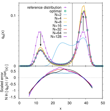
Figure 2: Optimal Bayesian ensemble refinement and Bayesian replica ensemble refinement for one-dimensional double well system with restraint on the mean, as indicated by the vertical black line. (Top) Marginalized distributions $q_{N}(x)$ from Bayesian replica ensemble refinement with $N$ replicas (lines) compared to the optimal Bayesian ensemble refinement solution $p^{\mathrm{(opt})\!}(x)$ (open squares) and to the reference distribution $p_{0}(x)$ (thin line with open circles). Arrows indicate changes relative to $p_{0}(x)$. (Bottom) Error $N[\ln q_{N}(x)-\ln p^{\mathrm{(opt})\!}(x)]$ in $\ln q_{N}(x)$ scaled by the number of replicas $N$. Part of the scatter is a reflection of the stochastic Monte Carlo sampling of the Bayesian distributions $q_{N}(x)$.

Convergence of Bayesian replica ensemble refinement.

To examine the convergence of the Bayesian replica ensemble refinement with the number $N$ of replicas towards the optimal Bayesian ensemble refinement solution, we have performed Metropolis Monte Carlo simulations for a one-dimensional system defined by a double-well potential energy function $\beta U(x)=3[(x-a)^{2}-b^{2}]^{2}/b^{4}$ with $a=(M+1)/2$ and $b=(M+2)/4$. We have discretized the potential at $x=1,2,\ldots,M$ with $M=50$. The mean of the corresponding reference distribution $p_{0}(x)\propto\exp[-\beta U(x)]$ is at $\overline{x}=a=25.5$. In the ensemble refinement, we set the target half-way between the maximum and the upper minimum, at $Y=(6+5M)/8=32$. The resulting $\chi^{2}$ then becomes $\chi^{2}=(N^{-1}\sum_{\alpha=1}^{M}x_{\alpha}-Y)^{2}/\sigma^{2}$, with $\sigma$ set to one. Systems with $N=2,4,8,\ldots,128$ replicas were sampled with Monte Carlo simulations, and the distributions $q_{N}(x)$ averaged over all replicas calculated.

Figure 2 compares the resulting distributions $q_{N}(x)$ of $x$ from Bayesian replica ensemble refinement to $p^{\mathrm{(opt})\!}(x)$ from optimal Bayesian ensemble refinement. We find that the ensemble reweighted distributions shift contributions from the left well to the right well to match the target mean, but by and large retain the shape within each well of the potential $U(x)$ defining the reference distribution. The only exception is $N=2$, where the restraint on the mean effectively pulls one of the replicas out of the first minimum into the barrier region. We also find numerically that the distributions $q_{N}(x)$, averaged over all replicas $N$, converge asymptotically (for large $N$) to the optimal Bayesian ensemble refinement solution $p^{\mathrm{(opt})\!}(x)$ as $\ln q_{N}(x)\approx\ln p^{\mathrm{(opt})\!}(x)+f(x)/N$ for $N\geq 16$. Numerical results for the master curve $f(x)=N\ln[q_{N}(x)/p^{\mathrm{(opt})\!}(x)]$ are shown in the bottom panel of Figure 2 bottom; the actual error in an $N$-replica simulation is approximately $1/N$-th of $f(x)$. The probability density from Bayesian replica ensemble refinement thus appears to converge asymptotically as $1/N$ to the optimal Bayesian result, as in the first analytically tractable example above.

Convergence of EROS.

We have used the same model to examine the convergence of EROS in the case where $n$ representative configurations are drawn according to $p_{0}(x)$ and then reweighted according to Eq. (II.2). Specifically, we have drawn $n$ values of $x$ with replacement according to the Boltzmann distribution for the double-well potential with $M=50$. The resulting $n$ points, indexed as $\alpha(1),\ldots,\alpha(n)$, were then reweighted according to Eq. (II.2), with $w_{\alpha(i)}^{0}=1/n$ for all $i$. The resulting EROS weights were then averaged for each of the $M$ possible values of $x$,

$$p_{n}(x=x_{\alpha})=\left\langle\sum_{i=1}^{n}\delta_{\alpha,\alpha(i)}w_{\alpha(i)}^{(\mathrm{opt})}\right\rangle,$$ (44)

where $\langle\cdots\rangle$ indicates an average over repeated selections of samples of size $n$, and $\delta_{\alpha,\gamma}=1$ if $\alpha=\gamma$ and zero otherwise. In this way, we estimated the expected weight of configuration $\alpha$ in repeated EROS runs using $n$ representative ensembles.

In Figure 3, we show that the distribution $p_{n}(x=x_{\alpha})$ obtained by repeated reweighting indeed converges to the optimal Bayesian ensemble refinement result in the limit of large $n$. For the specific example, the error in $\ln p_{n}(x)$ scales as $1/n$. Interestingly, the relative error obtained for EROS samples of size $n$ is comparable to that of Bayesian replica ensemble refinement with $n$ replicas.

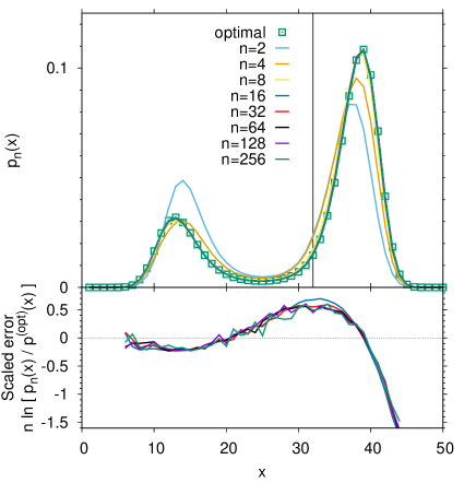
Figure 3: EROS and optimal Bayesian ensemble refinement for a one-dimensional double well system with restraint on the mean, as indicated by the vertical black line. (Top) Marginalized distributions $p_{n}(x)$ from EROS with $n$ configurations drawn according to $p_{0}$ (lines) compared to the optimal Bayesian ensemble refinement solution $p^{\mathrm{(opt})\!}(x)$ (open squares). (Bottom) Error $n[\ln p_{n}(x)-\ln p^{\mathrm{(opt})\!}(x)]$ in $\ln p_{n}(x)$ scaled by the sample size $n$. Part of the scatter is a reflection of the stochastic Monte Carlo sampling of configurations in EROS.

BioEn improves convergence by combining EROS and replica simulations.

We have also tested the BioEn combination of EROS and replica simulations to speed up convergence to the optimal Bayesian ensemble distribution. Figure 4 demonstrates the dramatic improvement achieved in the combined method for the model of Figures 2 and 3. After EROS reweighting of the configurations sampled in unbiased and biased runs with $N=2$, 4, and 8 replicas, we find that the significant systematic errors in the Bayesian replica ensemble distributions $q_{N}(x)$ disappear, and only small, primarily statistical errors remain.

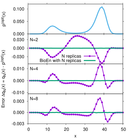
Figure 4: BioEn method applied to double-well system. The bottom three panels show the error $\Delta q_{N}(x)=q_{N}(x)-p^{\mathrm{(opt})\!}(x)$ in the ensemble distributions obtained from regular replica ensemble refinement with $N=2$, 4, and 8 replicas (purple line with symbols) relative to the optimal Bayesian ensemble distribution $p^{\mathrm{(opt})\!}(x)$ (shown in the top panel). Also shown is the error of the BioEn method combining EROS and replica refinement (green lines). Please note the change in scale of the vertical axes for different $N$. See Figure 2 for the error in $\ln q_{N}(x)$ without BioEn for larger numbers of replicas $N$.

III.2 Practical considerations

Combining common-property and ensemble-average refinement.

For simplicity, we have so far dealt separately with observables reporting on properties common to all configurations and on ensemble averages. However, these data can be combined readily within the above formalisms. In the respective posteriors, the likelihood terms according to Eqs. (8) and (14) simply have to be multiplied. The optimal Bayesian ensemble distribution then becomes

$$p^{\mathrm{(opt})\!}(\mathbf{x})\propto p_{0}(\mathbf{x})\exp{\left[-\sum_{i=1}^{m}\frac{\left[y_{i}(\mathbf{x})-y_{i}^{(\mathrm{obs})}\right]^{2}}{2\theta\sigma_{i}^{2}}\right]}$$

$$\times\exp{\left[-\sum_{i=m+1}^{M}\frac{y_{i}(\mathbf{x})\left[\int d\mathbf{x}^{\prime}p^{\mathrm{(opt})\!}(\mathbf{x}^{\prime})y_{i}(\mathbf{x}^{\prime})-Y_{i}^{(\mathrm{obs})}\right]}{\theta\sigma_{i}^{2}}\right]},$$

for $m$ restraints on common properties, and $M-m$ restraints on ensemble averages. Equation (III.2) is a combination of Eqs. (12) and (II.2). An analogous expression generalizes Eq. (II.2) for the discrete case.

Data from single-molecule experiments.

Data from single-molecule experiments can be incorporated in the different refinement procedures. In principle, one could even fit the data individually, one molecule at a time, using single-copy refinement. In a more practical approach, one can use the techniques of ensemble refinement to fit the single-molecule data lumped together in a way that produces not just averages but also distributions of observables. An example are FRET efficiencies $E$ measured by single-molecule spectroscopy. As a basis for ensemble refinement,Boura et al. (2011, 2012) one can for instance determine FRET-efficiency histograms $H_{i}^{(\mathrm{obs})}\equiv H^{(\mathrm{obs})}(E_{i})$ from photon arrival trajectories and use the deviations between histogram counts calculated for an ensemble model, $H_{i}\equiv{\cal Y}_{i}[p(x)]$, and measured in experiment, $H_{i}^{(\mathrm{obs})}\equiv Y_{i}^{(\mathrm{obs})}$, to construct a $\chi^{2}$, with appropriate error models. With such a $\chi^{2}$, one can then use both EROS Boura et al. (2011, 2012) and Bayesian replica ensemble refinement.

Dynamic, time-dependent data such as NMR NOEs.

Many relevant observables are not just functions of a configuration, $y_{i}\equiv y_{i}(\mathbf{x})$, but depend also on the dynamics. Examples are the NOE intensity and other NMR relaxation parameters that depend on the rotational and translational dynamics of the spin system.Peter, Daura, and van Gunsteren (2001) Whereas it is outside of the scope of this article to refine an entire dynamical model to such data, we can make some progress in this direction by considering a reduced problem. Ignoring self-consistency issues, we can attempt to refine an ensemble of configurations $\mathbf{x}$ that evolve in time under the Hamiltonian of the molecular simulation energy function $U(\mathbf{x})$ defining the reference distribution $p_{0}(\mathbf{x})$, but are distributed according to $p^{\mathrm{(opt})\!}(\mathbf{x})$ instead of $p_{0}(\mathbf{x})$.

To calculate the observables associated with a particular configuration $\mathbf{x}$, one can use trajectory segments passing through $\mathbf{x}$. Each of the sample configurations $\mathbf{x}$ would then serve as an initial value, with Maxwell-Boltzmann velocities, for one or multiple trajectory segments of length $\tau/2$. To center the trajectories at $\mathbf{x}$ with respect to time, one can run trajectory pairs of length $\tau/2$, initiated from $\mathbf{x}$ with sign-inverted Maxwell-Boltzmann velocities, one running forward and the other running backward in time. Stitching the two segments together at $\mathbf{x}$, after sign-inverting the velocities of the backward segment, one obtains a continuous trajectory of length $\tau$ centered time-wise at $\mathbf{x}$. For each of these trajectories, the time-dependent observable $y_{i}=y_{i}[\mathbf{x}(t)|\mathbf{x}(0)=\mathbf{x};-\tau/2\leq t\leq\tau/2]$ can be calculated, possibly averaged by repeated runs over different choices of initial Maxwell-Boltzmann velocities. The $y_{i}$ calculated in this manner can be treated as simple functions of $\mathbf{x}=\mathbf{x}(0)$ to enter the $\chi^{2}$ in the same way as static data. The trajectory length $\tau$ should be set such that the $y_{i}$ can be calculated with reasonable accuracy (i.e., as multiples of the relevant correlation times). After refinement, one obtains an ensemble of configurations that jointly account for the time-dependent observables yet stay close to the reference distribution. We note that (possibly overlapping) trajectory segments could also be obtained from long equilibrium trajectories, or even from $N$-replica simulations.

As the simplest approach of refining also the actual dynamics, one can perform in addition time scaling, $t\mapsto\alpha t$, which could for instance account for incorrect viscosities of the water model used in the molecular dynamics simulations. The time-scale parameter $\alpha$ can then be optimized as well in the ensemble refinement.

Solving the EROS equations.

One can obtain the EROS weights in Eq. (II.2) by numerical minimization of ${\cal L}$ in Eq. (II.2), which can be accomplished by a variety of techniques with and without gradient calculations. Alternatively, one can solve Eq. (II.2) directly, for instance by iteration until self-consistency is achieved. A possible route is to start from the weights $w_{\alpha}^{\mathrm{(opt})\!}\approx w_{\alpha}^{0}$ in the reference distribution, and then iterate Eq. (II.2) to get an updated estimate of $w_{\alpha}^{\mathrm{(opt})\!}$. This procedure can be repeated until the change in old and new approximations drops below a chosen threshold. We found that mixing the old and new approximations geometrically, as ${(w^{(\mathrm{old})}_{\alpha})}^{x}{(w_{\alpha}^{(\mathrm{new})})}^{(1-x)}$ with $0<x<1$, led to stable fixed-point iterations. The mixing parameter $x$ controls stability ($x\approx 1$) and speed ($x\approx 0$). We further improved the stability and convergence behavior by starting at a large value of $\theta$, where the deviations from the reference distribution $w_{\alpha}^{0}$ are small, and then reducing $\theta$ in repeated fixed-point iterations to sweep out a broad $\theta$ range. The resulting EROS refinements for different $\theta$ can help us in the choice of $\theta$, as discussed next.

Choosing the confidence factor $\theta$.

The Bayesian ensemble refinement methods described here contain one free parameter, the factor $\theta$ that enters the prior and quantifies the level of confidence one has in the reference probability density $p_{0}(\mathbf{x})$. Large values of $\theta$ express high confidence (for instance, if one uses a well-tested atomistic force field instead of a more approximate coarse-grained representation, both being well sampled). Whereas formally, one would choose $\theta$ before refinement, in practice one may want to readjust this choice after the fact to achieve a better balance between reference distribution and data. By reporting the chosen $\theta$ and the corresponding Kullback-Leibler divergence between reference and optimal distribution, the inference process becomes transparent.

Akin to L-curve selection in other regularization approaches to inverse problems,Hansen and O’Leary (1993) one can find an appropriate value of $\theta$ by plotting the Kullback-Leibler divergence (relative entropy) $S_{\mathrm{KL}}=-\sum_{\alpha}w_{\alpha}^{\mathrm{(opt})\!}\ln({w_{\alpha}^{\mathrm{(opt})\!}}/{w_{\alpha}^{0}})$ against the $\chi^{2}$ obtained in EROS reweighting for different values of $\theta$. As discussed above, EROS reweighting can (and should) be performed even when Bayesian replica ensemble refinement is used to obtain the configurations to avoid finite-$N$ effects. The value of $\beta^{-1}S_{\mathrm{KL}}$ can then be interpreted as the average error in the energy function $U(\mathbf{x})$ used to define the reference distribution, since by definition $S_{\mathrm{KL}}=\beta\int d\mathbf{x}\,p^{\mathrm{(opt})\!}(\mathbf{x})\,[U^{(\mathrm{opt})}(\mathbf{x})-U(\mathbf{x})]$ for $p^{\mathrm{(opt})\!}(\mathbf{x})\propto\exp[-\beta U^{(\mathrm{opt})}(\mathbf{x})]$, given that the additive constant in $U^{(\mathrm{opt})}(\mathbf{x})$ is chosen such that the partition functions (and thus free energies) of the optimal and reference distribution are identical, $\int d\mathbf{x}\exp[-\beta U^{(\mathrm{opt})}(\mathbf{x})]=\int d\mathbf{x}\exp[-\beta U(\mathbf{x})]$. This allows one to choose a $\theta$ value on the basis of expectations concerning the magnitude of this error.Rozycki, Kim, and Hummer (2011) Conversely, one can also take a more pragmatic approach and choose a value of $\theta$ at the kink of the $S_{\mathrm{KL}}$-versus-$\chi^{2}$ curve, where a further decrease in $\theta$ does not produce a significant improvement in the fit quality but causes a large deviation from the reference distribution, as measured by $S_{\mathrm{KL}}$. This approach is taken in the MERA web server for the refinement of peptide Ramachandran maps against NMR data.Mantsyzov et al. (2014, 2015) There one accepts a $\chi^{2}$ a certain percentage point (say, 25 %) above the minimal $\chi^{2}$ obtained for $\theta\approx 0$.

Finally, the confidence parameter $\theta$ can also be treated as a nuisance parameter with an uninformative prior, $p(\theta)\propto 1/\theta$ for $\theta>0$. One could include $\theta$ in the maximization of the posterior or attempt to integrate it out in a weighted average over ensembles obtained for fixed $\theta$.

IV Conclusions

We have described different Bayesian approaches to ensemble refinement, established their interrelations, and shown how they can be applied to experimental data. The Bayesian approaches allow one to integrate a wide variety of experiments, including experiments reporting on properties common to all configurations and on averages over the entire ensemble. We started from a Bayesian formulation in which the posterior is a functional that ranks the quality of the configurational distributions. We then derived expressions for the optimal probability distribution in configuration space. For discrete configurations, we found that this optimal distribution is identical to that obtained by the EROS model.Rozycki, Kim, and Hummer (2011) To perform ensemble refinement “on the fly”, or to enhance the sampling of relevant configurations in cases where the reference distribution and the optimal ensemble density have limited overlap, we considered replica-simulation methods in which a restraint is imposed through a biasing potential that acts on averages over all replicas. We showed using a mean-field treatment that to obtain a size-consistent result, the biasing potential has to be scaled by the number $N$ of replicas, i.e., the restraint has to become stiffer as more replicas are included. Then, the Bayesian replica ensemble refinement converges to the optimal Bayesian ensemble refinement in the limit of infinitely many replicas, $N\rightarrow\infty$. This result clarifies the need to scale the biasing potential, which arises also in maximum entropy treatments with strict constraints,Cavalli, Camilloni, and Vendruscolo (2013a, b); Roux and Weare (2013) with the number of replicas $N$ to obtain a size-consistent result. An adaptive method, as described in the Appendix, provides a possible alternative to replica-based approaches.

The BioEn approach combines the replica and EROS refinement methods. The replica simulations are used to create an enriched sample of configurations. A free-energy calculation is used to determine the appropriate weights according to the reference ensemble. The optimal weights according to Bayesian ensemble refinement are then determined by EROS. This combined approach addresses the shortcomings of either method, i.e., the need to work with relatively small $N$ in replica simulations, and potentially limited overlap of reference and optimized distribution in EROS. Using free-energy reweighting methods, it may also be possible to include configurations from other types of ensemble-biased simulations, including those designed to satisfy measurements exactly.Camilloni, Cavalli, and Vendruscolo (2013); Hansen et al. (2014); Marinelli and Faraldo-Gomez (2015) Because of the flexibility and expected rapid convergence, the BioEn method combining Bayesian replica and EROS refinement should perform well in practical applications.

In two examples that are analytically tractable and one requiring numerical calculations, we demonstrated the equivalence of the different methods in the appropriate limits. We also studied the convergence properties of Bayesian replica simulations with the number of replicas $N$, and of EROS reweighting with the sample size $n$. Our examples showed similar convergence of the log-probability of the two refinement approaches to the optimal limit as $1/N$ and $1/n$, respectively.

The BioEn approach also addresses a major issue in Bayesian ensemble refinement, namely the choice of $\theta$. This parameter enters the prior to express our confidence in the reference distribution. We find that in the optimal Bayesian ensemble distributions, a change in $\theta$ is simply equivalent to a uniform scaling of all squared Gaussian errors $\sigma_{i}^{2}$. Since EROS reweighting is usually orders of magnitudes less costly than sampling multiple replicas in coupled molecular simulations, one can efficiently obtain estimates of the relative entropy $S_{\mathrm{KL}}$ for different $\theta$. From plots of $S_{\mathrm{KL}}$ against $\chi^{2}$ one can make an educated choice of $\theta$, as in other regularization approaches to inverse problems.Hansen and O’Leary (1993)

Finally, the reweighting of individual structures, either directly using EROS or in the combined approach, should prove useful in the optimization of potential energy functions by fitting them to experimental data (see, e.g., Refs. Norgaard, Ferkinghoff-Borg, and Lindorff-Larsen, 2008; Li and Brueschweiler, 2011; Wang, Chen, and Voorhis, 2013). If one has a good understanding of the sources of the errors in the energy surface $U(\mathbf{x})$, parameters in $U$ can be fitted directly, as was done, e.g., for the star force fields of proteins Best and Hummer (2009) and for RNA.Chen and García (2013) At the other extreme, Bayesian approaches have been used before to infer entire energy functions.Habeck (2014) Here, we suggest to concentrate on the change in weight of structures $\mathbf{x}_{\alpha}$, i.e., $\ln w_{\alpha}^{\mathrm{(opt})\!}/w_{\alpha}^{0}=-\beta\Delta U_{\alpha}+\mathit{const.}$, which defines the required change $\Delta U_{\alpha}$ in the potential energy to match experiment. By examining the correlation of this force field error $\Delta U_{\alpha}$ with elements of the force field (e.g., peptide dihedral angles Best and Hummer (2009) or base stacking interactions Chen and García (2013)), it might be possible to identify sources of the error and then correct for them.

It is important to emphasize that a number of assumptions enter the ensemble refinement procedure. The central (and declared!) assumption is that of a reference distribution. Here it may be possible to use combinations of multiple potential energy functions $u_{k}(\mathbf{x})$, representing different force fields or conditions $k$, that jointly cover the relevant phase space better than any potential alone. One way to mix such potentials is by using a multistate model,Best, Chen, and Hummer (2005) $U(\mathbf{x})=-\gamma^{-1}\ln\sum_{k}\exp[-\gamma u_{k}(\mathbf{x})+\epsilon_{k}]$, where $\gamma$ is the mixing “temperature” and $\epsilon_{k}$ are energy offsets that weight the different force fields. Another important challenge is that one has to estimate errors both in the measurements and in the calculation of the observables. Procedures to account for uncertainties in the error estimates have been developed.Rieping, Habeck, and Nilges (2005) Within the present framework, one could include error distributions in the maximization of the log-posterior, or average over optimal solutions obtained for different errors. In addition, in many cases the Gaussian error model may not be appropriate. As discussed, to handle more general error models, one can substitute the log-likelihood $\ln{\cal P}[\mathrm{data}|p(\mathbf{x})]$ for $-\chi^{2}/2$ in ${\cal P}[p(\mathbf{x})|\mathrm{data}]$.

Overall, we expect our exploration of different Bayesian ensemble refinement approaches to serve both as a basis for practical applications and as a starting point for further investigations. In particular, we have here not considered an orthogonal refinement approach in which one seeks to represent the ensemble by a minimal set of structures.Boura et al. (2011); Berlin et al. (2013); Cossio and Hummer (2013); Pelikan, Hura, and Hammel (2009) As we had shown before, EROS and minimal ensemble refinement, properly interpreted, can give consistent results.Francis et al. (2011) However, the relation of the different methods is not well understood, e.g., concerning the limiting behavior for large sample sizes.

Appendix A Adaptive sampling of optimal Bayesian distribution without replicas

We define probability densities of the observables alone by integrating out all other degrees of freedom,

$$P_{0}(\mathbf{y}) = \int d\mathbf{x}\,p_{0}(\mathbf{x})\prod_{i=1}^{M}\delta[y_{i}-y_{i}(\mathbf{x})],$$ (46)

$$P(\mathbf{y}) = \int d\mathbf{x}\,p(\mathbf{x})\prod_{i=1}^{M}\delta[y_{i}-y_{i}(\mathbf{x})].$$ (47)

According to Eqs. (II.2) and (22), these two distributions are related to each other,

$$P(\mathbf{y})\propto P_{0}(\mathbf{y})\exp{\left(-\frac{1}{\theta}\sum_{i,j=1}^{M}y_{i}(\bm{\Sigma}^{-1})_{ij}f_{j}\right)}$$ (48)

for possibly correlated Gaussian errors, where the generalized forces $f_{j}$ have to be determined self-consistently such that

$$f_{j}=\int d\mathbf{y}\,P(\mathbf{y})y_{j}-Y_{j}^{(\mathrm{obs})}=\langle y_{j}\rangle-Y_{j}^{(\mathrm{obs})}.$$ (49)

As a consequence, $p(\mathbf{x})\propto p_{0}(\mathbf{x})\exp[-\theta^{-1}\mathbf{y}^{T}(\mathbf{x})\bm{\Sigma}^{-1}\mathbf{f}]$ where superscript $T$ indicates the transpose in vector-matrix notation. The biasing potential thus assumes a functional form linear in the $y_{i}(\mathbf{x})$, as seen in standard maximum entropy approaches (see, e.g., Refs. Pitera and Chodera, 2012; Beauchamp, Pande, and Das, 2014; White and Voth, 2014), but the generalized forces $f_{i}$ take on different values here. We also note that the forces $f_{j}$ defining the optimal distribution can be interpreted mechanically. With Eq. (48) one finds that the mean force trying to “restore” the reference distribution, $\mathbf{F}^{(\mathrm{ref})}\equiv\int d\mathbf{y}\,P(\mathbf{y})\partial[-\ln P_{0}(\mathbf{y})]/\partial\mathbf{y}=-\theta^{-1}\bm{\Sigma}^{-1}\mathbf{f}$, is exactly balanced by the mean force to fit the data, $\mathbf{F}^{(\mathrm{fit})}\equiv\int d\mathbf{y}\,P(\mathbf{y})\partial(\chi^{2}/2)/\partial\mathbf{y}=\bm{\Sigma}^{-1}\mathbf{f}$, up to a factor $\theta$, with $\chi^{2}$ from Eq. (5) with $Y_{j}^{(\mathrm{obs})}$ instead of $y_{j}^{(\mathrm{obs})}$.

Formally, the $f_{j}$ can be obtained by solving $M$ coupled nonlinear equations. We define generating functions $\phi_{0}(\mathbf{z})\equiv\int d\mathbf{y}\,P_{0}(\mathbf{y})\exp(\mathbf{y}\cdot\mathbf{z})=\int d\mathbf{x}\,p_{0}(\mathbf{x})\exp[\sum_{i}y_{i}(\mathbf{x})z_{i}]$ and $\phi(\mathbf{z})\equiv\int d\mathbf{y}\,P(\mathbf{y})\exp(\mathbf{y}\cdot\mathbf{z})=\int d\mathbf{x}\,p(\mathbf{x})\exp[\sum_{i}y_{i}(\mathbf{x})z_{i}]$, assuming that the integrals exist. Multiplying Eq. (48) by $\exp(\mathbf{y}\cdot\mathbf{z})$ and integrating over $\mathbf{y}$, we obtain

$$\phi(\mathbf{z})=\frac{\phi_{0}\left[\mathbf{z}-\theta^{-1}(\bm{\Sigma}^{-1})\mathbf{f}\right]}{\phi_{0}\left[-\theta^{-1}(\bm{\Sigma}^{-1})\mathbf{f}\right]},$$ (50)

where the denominator ensures normalization, $\phi(0)=1$. With $\langle y_{j}\rangle=\left.\partial\phi(\mathbf{z})/{\partial z_{j}}\right|_{\mathbf{z}=0}$, Eq. (49) for the vector of forces $\mathbf{f}$ becomes satisfy

$$\mathbf{f}=\left.\frac{\partial\ln\phi_{0}\left[\mathbf{z}-\theta^{-1}(\bm{\Sigma}^{-1})\mathbf{f}\right]}{\partial\mathbf{z}}\right|_{\mathbf{z}=0}-\mathbf{Y}^{(\mathrm{obs})},$$ (51)

where $\ln\phi_{0}(\mathbf{z})$ is the cumulant generating function of the reference distribution of observables.

In cases where the equations cannot be solved directly, one can determine the force-vector $\mathbf{f}$ adaptively. In the following, we present a simple algorithm that can be combined with existing simulation procedures. This approach is related to that of White and Voth,White and Voth (2014) in which an adaptive gradient-based method is used to construct a distribution in which the $y_{j}$-averages exactly match $Y_{j}^{(\mathrm{obs})}$. Here, by contrast, we include measurement errors and thus do not demand exact agreement with the observed values. Instead, the $f_{j}$ have to be determined self-consistently to satisfy Eq. (49). In our adaptive optimization, we adjust the generalized forces $f_{j}$ “on the fly” according to the running averages of the $y_{j}$,

$$\mathbf{f}(t)=\frac{1}{t}\int_{0}^{t}d\tau\,\mathbf{y}[\mathbf{x}(\tau)]-\mathbf{Y}^{(\mathrm{obs})},$$ (52)

with initial value $\mathbf{f}(0)=\mathbf{y}[\mathbf{x}(0)]$. Here, the trajectory $\mathbf{x}(t)$ evolves according to the time-dependent potential energy $U(\mathbf{x})+\mathbf{y}(\mathbf{x})\bm{\Sigma}^{-1}\mathbf{f}(t)/\theta$. We note that by extending the phase space to include both $\mathbf{x}$ and $\mathbf{f}$, this algorithm can be cast in a Markovian form. If $L_{f}$ is the Liouville evolution operator for the phase space density of $\mathbf{x}$ according to the molecular dynamics or Monte Carlo simulation protocol and potential $U(\mathbf{x})+\mathbf{y}(\mathbf{x})\bm{\Sigma}^{-1}\mathbf{f}/\theta$ with fixed $\mathbf{f}$, then the extended phase space density $\rho=\rho(\mathbf{x},\mathbf{f},t)$ satisfies a Markovian Liouville-type evolution equation

$$\frac{\partial\rho}{\partial t}=\left[L_{f}+\frac{1}{t}\frac{\partial}{\partial\mathbf{f}}\left(\mathbf{f}+\mathbf{Y}^{(\mathrm{obs})}-\mathbf{y}(\mathbf{x})\right)\right]\rho.$$ (53)

Using this relation, one can show that for the Gaussian example in the main text, with the mean as observable and overdamped diffusion for the dynamics of $\mathbf{x}$, the adaptive sampling is globally converging to the optimal Bayesian ensemble distribution. For the example in Fig. 2, with Monte Carlo sampling of $x$, we observed convergence numerically.

We note that in the adaptive determination of the generalized forces $f_{j}$ defining the posterior distribution, variants of Eq. (52) are possible. In particular, one can average between an initial guess $\mathbf{f}_{0}$ and the evolving mean, e.g., as $\mathbf{f}(t)=w(t)\mathbf{f}_{0}+[1-w(t)][t^{-1}\int_{0}^{t}d\tau\,\mathbf{y}[\mathbf{x}(\tau)]-\mathbf{Y}^{(\mathrm{obs})}]$, where $w(t)$ is a weight function that decreases to zero with time, e.g., $w(t)=\exp(-t/t_{0})$ for a suitably chosen relaxation time $t_{0}$.

References

- Boomsma, Ferkinghoff-Borg, and Lindorff-Larsen (2014) W. Boomsma, J. Ferkinghoff-Borg, and K. Lindorff-Larsen, PLoS Comp. Biology 10 (2014).
- Sali et al. (2015) A. Sali, H. M. Berman, T. Schwede, J. Trewhella, G. Kleywegt, S. K. Burley, J. Markley, H. Nakamura, P. Adams, A. M. J. J. Bonvin, W. Chiu, M. Peraro, F. Di Maio, T. E. Ferrin, K. Grünewald, A. Gutmanas, R. Henderson, G. Hummer, K. Iwasaki, G. Johnson, C. Lawson, J. Meiler, M. A. Marti-Renom, G. Montelione, M. Nilges, R. Nussinov, A. Patwardhan, J. Rappsilber, R. J. Read, H. Saibil, G. F. Schröder, C. D. Schwieters, C. A. M. Seidel, D. Svergun, M. Topf, E. L. Ulrich, S. Velankar, and J. D. Westbrook, Structure 23, 1156 (2015).
- Boura et al. (2011) E. Boura, B. Rozycki, D. Z. Herrick, H. S. Chung, J. Vecer, W. A. Eaton, D. S. Cafiso, G. Hummer, and J. H. Hurley, Proc. Natl. Acad. Sci. U.S.A. 108, 9437 (2011).
- Ward, Sali, and Wilson (2013) A. B. Ward, A. Sali, and I. A. Wilson, Science 339, 913 (2013).
- Camilloni and Vendruscolo (2014) C. Camilloni and M. Vendruscolo, J. Am. Chem. Soc. 136, 8982 (2014).
- Fisher, Huang, and Stultz (2010) C. K. Fisher, A. Huang, and C. M. Stultz, J. Am. Chem. Soc. 132, 14919 (2010).
- Fisher and Stultz (2011) C. K. Fisher and C. M. Stultz, Curr. Opin. Struct. Biol. 21, 426 (2011).
- Sanchez-Martinez and Crehuet (2014) M. Sanchez-Martinez and R. Crehuet, Phys. Chem. Chem. Phys. 16, 26030 (2014).
- Dedmon et al. (2005) M. M. Dedmon, K. Lindorff-Larsen, J. Christodoulou, M. Vendruscolo, and C. M. Dobson, J. Am. Chem. Soc. 127, 476 (2005).
- Mantsyzov et al. (2014) A. B. Mantsyzov, A. S. Maltsev, J. Ying, Y. Shen, G. Hummer, and A. Bax, Protein Sci. 23, 1275 (2014 2014 2014).
- Mantsyzov et al. (2015) A. B. Mantsyzov, Y. Shen, J. Lee, G. Hummer, and A. Bax, J. Biomol. NMR , 1 (2015).
- Schröder (2015) G. F. Schröder, Curr. Opin. Struct. Biol. 31, 20 (2015).
- Rozycki, Kim, and Hummer (2011) B. Rozycki, Y. C. Kim, and G. Hummer, Structure 19, 109 (2011).
- Francis et al. (2011) D. M. Francis, B. Rozycki, D. Koveal, G. Hummer, R. Page, and W. Peti, Nature Chem. Biology 7, 916 (2011).
- Scheek et al. (1991) R. M. Scheek, A. E. Torda, J. Kemmink, and W. F. van Gunsteren, NATO Advanced Science Institutes Series Series A Life Sciences 225, 209 (1991).
- Lange et al. (2008) O. F. Lange, N. A. Lakomek, C. Fares, G. F. Schröder, K. F. A. Walter, S. Becker, J. Meiler, H. Grubmüller, C. Griesinger, and B. L. de Groot, Science 320, 1471 (2008).
- Olsson et al. (2014) S. Olsson, B. R. Vögeli, A. Cavalli, W. Boomsma, J. Ferkinghoff-Borg, K. Lindorff-Larsen, and T. Hamelryck, J. Chem. Theory Comput. 10, 3484 (2014).
- Boura et al. (2012) E. Boura, B. Rozycki, H. S. Chung, D. Z. Herrick, B. Canagarajah, D. S. Cafiso, W. A. Eaton, G. Hummer, and J. H. Hurley, Structure 20, 874 (2012).
- Cossio and Hummer (2013) P. Cossio and G. Hummer, J. Struct. Biol. 184, 427 (2013).
- Schneidman-Duhovny, Pellarin, and Sali (2014) D. Schneidman-Duhovny, R. Pellarin, and A. Sali, Curr. Opin. Struct. Biol. 28, 96 (2014).
- MacKay (2003) D. J. C. MacKay, Information Theory, Inference, and Learning Algorithms (Cambridge University Press, Cambridge, UK, 2003).
- Rieping, Habeck, and Nilges (2005) W. Rieping, M. Habeck, and M. Nilges, Science 309, 303 (2005).
- Crooks (2007) G. E. Crooks, Phys. Rev. E 75, 041119 (2007).
- Gull and Daniell (1978) S. F. Gull and G. J. Daniell, Nature 272, 686 (1978).
- Jaynes (1982) E. T. Jaynes, Proc. IEEE 70, 952 (1982).
- Press et al. (1992) W. H. Press, S. A. Teukolsky, W. T. Vetterling, and B. P. Flannery, “Numerical recipes in FORTRAN,” (Cambridge University Press, Cambridge, U.K., 1992) Chap. 18.7, 2nd ed.
- Pitera and Chodera (2012) J. W. Pitera and J. D. Chodera, J. Chem. Theory Comput. 8, 3445 (2012).
- White and Voth (2014) A. D. White and G. A. Voth, J. Chem. Theory Comput. 10, 3023 (2014).
- White, Dama, and Voth (2015) A. D. White, J. F. Dama, and G. A. Voth, J. Chem. Theory Comput. 11, 2451 (2015).
- Beauchamp, Pande, and Das (2014) K. A. Beauchamp, V. S. Pande, and R. Das, Biophys. J. 106, 1381 (2014).
- Kim and Prestegard (1989) Y. Kim and J. H. Prestegard, Biochemistry 28, 8792 (1989).
- Kuriyan et al. (1991) J. Kuriyan, K. Osapay, S. K. Burley, A. T. Brunger, W. A. Hendrickson, and M. Karplus, Proteins Struct. Funct. Genet. 10, 340 (1991).
- Best and Vendruscolo (2004) R. B. Best and M. Vendruscolo, J. Am. Chem. Soc. 126, 8090 (2004).
- Lindorff-Larsen et al. (2005) K. Lindorff-Larsen, R. B. Best, M. A. Depristo, C. M. Dobson, and M. Vendruscolo, Nature 433, 128 (2005).
- Cavalli, Camilloni, and Vendruscolo (2013a) A. Cavalli, C. Camilloni, and M. Vendruscolo, J. Chem. Phys. 138, 094112 (2013a).
- Cavalli, Camilloni, and Vendruscolo (2013b) A. Cavalli, C. Camilloni, and M. Vendruscolo, J. Chem. Phys. 139, 169903 (2013b).
- Bonomi et al. (2015) M. Bonomi, C. Camilloni, A. Cavalli, and M. Vendruscolo, “Metainference: A Bayesian inference method for heterogeneous systems,” http://arxiv.org/abs/1509.05684 (2015).
- Roux and Weare (2013) B. Roux and J. Weare, J. Chem. Phys. 138, 084107 (2013).
- Rosta et al. (2011) E. Rosta, M. Nowotny, W. Yang, and G. Hummer, J. Am. Chem. Soc. 133, 8934 (2011).
- Shirts and Chodera (2008) M. R. Shirts and J. D. Chodera, J. Chem. Phys. 129, 124105 (2008).
- Souaille and Roux (2001) M. Souaille and B. Roux, Comp. Phys. Comm. 135, 40 (2001).
- Peter, Daura, and van Gunsteren (2001) C. Peter, X. Daura, and W. F. van Gunsteren, J. Biomol. NMR 20, 297 (2001).
- Hansen and O’Leary (1993) P. C. Hansen and D. P. O’Leary, SIAM J. Sci. Comput. 14, 1487 (1993).
- Camilloni, Cavalli, and Vendruscolo (2013) C. Camilloni, A. Cavalli, and M. Vendruscolo, J. Chem. Theory Comput. 9, 5610 (2013).
- Hansen et al. (2014) N. Hansen, F. Heller, N. Schmid, and W. F. van Gunsteren, J. Biomol. NMR 60, 169 (2014).
- Marinelli and Faraldo-Gomez (2015) F. Marinelli and J. D. Faraldo-Gomez, Biophys. J. 108, 2779 (2015).
- Norgaard, Ferkinghoff-Borg, and Lindorff-Larsen (2008) A. B. Norgaard, J. Ferkinghoff-Borg, and K. Lindorff-Larsen, Biophys. J. 94, 182 (2008).
- Li and Brueschweiler (2011) D. W. Li and R. Brueschweiler, J. Chem. Theory Comput. 7, 1773 (2011).
- Wang, Chen, and Voorhis (2013) L.-P. Wang, J. Chen, and T. Van Voorhis, J. Chem. Theory Comput. 9, 452 (2013).
- Best and Hummer (2009) R. B. Best and G. Hummer, J. Phys. Chem. B 113, 9004 (2009).
- Chen and García (2013) A. A. Chen and A. E. García, Proc. Natl. Acad. Sci. U.S.A. 110, 16820 (2013).
- Habeck (2014) M. Habeck, Phys. Rev. E 89, 052113 (2014).
- Best, Chen, and Hummer (2005) R. B. Best, Y.-G. Chen, and G. Hummer, Structure 13, 1755 (2005).
- Berlin et al. (2013) K. Berlin, C. A. Castaneda, D. Schneidman-Duhovny, A. Sali, A. Nava-Tudela, and D. Fushman, J. Am. Chem. Soc. 135, 16595 (2013).
- Pelikan, Hura, and Hammel (2009) M. Pelikan, G. L. Hura, and M. Hammel, Gen. Phys. Biophys. 28, 174 (2009).