On the self-sustained nature of large-scale motions in turbulent Couette flow

Abstract

Large-scale motions in wall-bounded turbulent flows are frequently interpreted as resulting from an aggregation process of smaller-scale structures. Here, we explore the alternative possibility that such large-scale motions are themselves self-sustained and do not draw their energy from smaller-scale turbulent motions activated in buffer layers. To this end, it is first shown that large-scale motions in turbulent Couette flow at ${\rm Re}=2150$ self-sustain even when active processes at smaller scales are artificially quenched by increasing the Smagorinsky constant $C_{s}$ in large eddy simulations. These results are in agreement with earlier results on pressure driven turbulent channels. We further investigate the nature of the large-scale coherent motions by computing upper and lower-branch nonlinear steady solutions of the filtered (LES) equations with a Newton-Krylov solver, and find that they are connected by a saddle-node bifurcation at large values of $C_{s}$. Upper branch solutions for the filtered large scale motions are computed for Reynolds numbers up to ${\rm Re}=2187$ using specific paths in the ${\rm Re}-C_{s}$ parameter plane and compared to large-scale coherent motions. Continuation to $C_{s}=0$ reveals that these large-scale steady solutions of the filtered equations are connected to the Nagata-Clever-Busse-Waleffe branch of steady solutions of the Navier-Stokes equations. In contrast, we find it impossible to connect the latter to buffer layer motions through a continuation to higher Reynolds numbers in minimal flow units.

1 Introduction

1.1 Streaky motions in wall-bounded turbulent flows

One of the most robust features observed in wall-bounded turbulent shear flows is the presence of quasi-streamwise streaks, i.e. narrow streamwise regions where the streamwise velocity is larger or smaller than its mean value. The flow visualizations of Kline et al. (1967) revealed that the near-wall region of turbulent boundary layers is very active and is populated by streamwise streaks in a spanwise quasi-periodic pattern. The average spanwise streak-spacing in the viscous sublayer and the buffer layer scales in wall units and corresponds approximately to $\lambda_{z}^{+}=100$ (Kline et al., 1967; Smith & Metzler, 1983). This spacing has been confirmed by the first direct numerical simulation of channel flow at $Re_{\tau}\approx 180$ by Kim et al. (1987), which also revealed the existence of counter-rotating quasi-streamwise vortices.

Streaky motions also exist at much larger scales. It has long been known that in turbulent flows the outer region is dominated by large-scale motions (LSM) with dimensions of the order of the outer length scale $h$ (e.g. the channel half-width or the boundary layer $\delta_{99}$ thickness) often separated by regions of non-turbulent fluid (Corrsin & Kistler, 1954; Kovasznay et al., 1970; Blackwelder & Kovasznay, 1972). More recently it has been realized that in addition to large-scale motions, ‘very large-scale motions’ (VLSM) exist with streamwise extensions at least fourfold those of the LSM. Large and very-large scale motions have been observed in turbulent pipe flow Kim & Adrian (1999), turbulent plane Poiseuille flow del Álamo & Jiménez (2003) and in the turbulent boundary layer Tomkins & Adrian (2003, 2005); Hutchins & Marusic (2007a). At high Reynolds numbers, these structures dominate the streamwise turbulent kinetic energy throughout the logarithmic region Tomkins & Adrian (2003, 2005), and modulate the cycles of near-wall structures Hutchins & Marusic (2007b); Mathis et al. (2009).

As far as turbulent Couette flow is concerned, Lee & Kim (1991) found large-scale motions in the form of quasi-steady large-scale coherent streaks and rolls in direct numerical simulations at ${\rm Re}=3000$ (where ${\rm Re}$ is based on the channel half-width $h$ and half of the velocity difference between the walls). These structures, of spanwise wavelength $\lambda_{z}\approx 4h$, occupied half of the spanwise size ($L_{z}=8.4h$) of the computational domain and its whole streamwise extension ($L_{x}=12.6h$). The existence of large-scale streaks was confirmed by the experiments of Tillmark & Alfredsson (1994). In order to understand whether the characteristics of these large-scale structures were affected by the size of the computational box, Komminaho et al. (1996) repeated the computations in a larger domain ($L_{x}=88h$ and $L_{z}=25.1h$) at ${\rm Re}=750$. They found large and very-large scale coherent streaks with the same spanwise wavelength ($\approx 4\,h$) as reported by Lee & Kim (1991), but more unsteady and extending more than $30h$ in the streamwise direction. They also found that resolving these structures is important to obtain accurate turbulent statistics. Kitoh et al. (2005), Tsukahara et al. (2006), Tsukahara et al. (2007) and Kitoh & Umeki (2008) also found large and very-large scale streaks at higher Reynolds numbers with typical spanwise spacings $\lambda_{z}\approx 4.2h-5h$ and streamwise lengths attaining $\lambda_{x}\approx 40h-60h$ for very-large scale motions.

1.2 Mechanisms sustaining streaky motions

There is now a relatively large consensus that streaky motions in the near-wall region rely on a self-sustained process. That the process is self-sustained was demonstrated by Jiménez & Moin (1991) who found that near-wall turbulence can be sustained in spanwise and streamwise periodic numerical domains as small as $L_{x}^{+}\times L_{z}^{+}\approx(250-300)\times 100$, showing that the motions in the viscous region are sustained independently from motions at larger scales. Hamilton et al. (1995) and Waleffe (1995) decomposed this nonlinear self-sustained process into three basic mechanisms: the lift-up effect which amplifies quasi-streamwise vortices into quasi-streamwise streaks, the amplification of sinuous modes supported by the streaks, and the streaks breakdown supporting the regeneration of the vortices. The lift-up is associated with the redistribution of streamwise momentum by counter-rotating, spanwise periodic quasi-streamwise vortices immersed in a basic shear flow. This redistribution leads to the transient amplification of high-velocity and low-velocity streamwise streaks (Moffatt, 1967; Ellingsen & Palm, 1975; Landahl, 1980, 1990; Schmid & Henningson, 2001). When the streaks reach sufficiently large amplitudes they become unstable to secondary perturbations via an inflectional, typically sinuous, instability (Waleffe, 1995; Reddy et al., 1998). As this secondary instability is subcritical, sinuous modes can also develop on top of streaks of amplitude smaller than the critical one (Schoppa & Hussain, 2002; Cossu et al., 2011). The breakdown of streamwise streaks finally leads to the regeneration of streamwise vorticity via nonlinear mechanisms. For the process to be self-sustained, the Reynolds number and the spanwise length of the box need to be large enough to allow for sufficient energy amplification by the lift-up effect and the streamwise length needs to be large enough to allow the secondary instability to be sufficiently amplified.

There is less consensus on the origin of large-scale motions. Early investigations showed that these motions contain a number of smaller scale structures which have been interpreted as hairpin vortices (Falco, 1977; Head & Bandyopadhay, 1981). Motions at large scales have therefore been interpreted as generated by the mutual vortical induction (Zhou et al., 1999; Adrian et al., 2000) and merger and growth of hairpins ultimately originating from the near-wall region (Tomkins & Adrian, 2003; Adrian, 2007). The idea that large-scale motions originate from motions at smaller scales is often implied in structural models of the logarithmic layer (Perry & Chong, 1982, and following extensions). As for very large-scale motions, it has been proposed that they result from the streamwise concatenation of large-scale motions (see e.g. Kim & Adrian, 1999; Guala et al., 2006; Dennis & Nickels, 2011). From a different perspective, Toh & Itano (2005) conjectured the existence of a co-supporting cycle where near-wall structures sustain large-scale structures in plane Poiseuille flow. The common point of these theories is that large-scale streaky motions would not exist in the absence of the near-wall active cycle.

The idea that near-wall active motions are ultimately necessary to form large-scale motions is however challenged by a growing number of recent results. For instance, it has been shown that large-scale outer motions are not significantly influenced by the change of the near-wall dynamics induced by wall-roughness (Flores & Jiménez, 2006; Flores et al., 2007) which implies that they are not very sensitive to the near-wall cycle. Also, some studies cast doubts on the very idea that hairpin vortices are a prominent feature of high Reynolds number turbulence (see e.g. Jeong et al., 1997; Eitel-Amor et al., 2015). Indeed, an alternative explanation of the origin of large-scale motions is currently emerging, which conjectures that these motions are sustained by a mechanism similar to the self-sustained process (SSP) proposed by Hamilton et al. (1995). This self-sustained process has been identified in transitional flows but Hamilton et al. (1995) argue that the near-wall streaky motions identified by Kline et al. (1967) are based on the same mechanism. An essential ingredient of this emerging scenario is the existence of a ‘coherent lift-up effect’, which would allow coherent large-scale motions to extract energy from the mean flow. That this coherent lift-up effect exists was shown by del Álamo & Jiménez (2006), Pujals et al. (2009) and Cossu et al. (2009), who computed the optimal linear transient growth sustained by turbulent mean flow profiles using the eddy viscosity model of Reynolds & Hussain (1972). Following the same approach Hwang & Cossu (2010a, b) and Willis et al. (2010) showed that turbulent Poiseuille, Hagen-Poiseuille and plane Couette flows all bear very large amplifications of harmonic and stochastic forcing. These different investigations all show that coherent streamwise and quasi-streamwise streaks can be amplified starting from coherent streamwise and quasi-streamwise vortices. The most amplified spanwise scales have been shown to be in good agreement with the spanwise spacing of large-scale streaks in the outer region and the associated maximum amplifications have been shown to increase with the Reynolds number. Pujals et al. (2010) experimentally confirmed the existence of the spatially-coherent transient growth of artificially forced large-scale structures in the turbulent boundary layer.

The existence of a robust coherent lift-up effect and of a secondary instability of large-scale streaks (Park et al., 2011) are strong indications that a self-sustained process might be at work at large scales in turbulent flows. The confirmation of the existence of this process was given by Hwang & Cossu (2010c), who showed that large-scale motions can self-sustain even in the absence of smaller-scale processes active in the near-wall and logarithmic regions. In order to suppress the small-scale motions while preserving the dissipation associated with them, Hwang & Cossu (2010c) used a large eddy simulation (LES) filter without energy backscatter and artificially increased its cutoff characteristic length. In this way, they were able to show that when the near-wall motions are artificially quenched, motions with the usual scales of large-scale motions survive. These conclusions were later extended by Hwang & Cossu (2011) to intermediate flow units characteristic of motions in the logarithmic layer (Flores & Jiménez, 2010).

1.3 Goal of the present study

The scope of the present study is twofold. The first, most immediate, objective is to determine if large-scale motions are self-sustained also in turbulent plane Couette flow. This would provide the first confirmation of the findings of Hwang & Cossu (2010c) in a flow other than the pressure driven channel flow. For the sake of exposing the objectives of our study, we anticipate the result that large-scale motions are indeed also self-sustained in turbulent plane Couette flow.

As a second objective we would like to further investigate the nature of the process by which these large-scale motions do self-sustain by using methods borrowed from dynamical systems theory. In particular, the computation and analysis of invariant solutions of the Navier-Stokes equations has led to important progress in the understanding of subcritical transition in shear flows. A number of non-trivial steady state solutions have for instance been computed in plane Couette flow (Nagata, 1990; Clever & Busse, 1992, 1997; Waleffe, 1998, 2003; Gibson et al., 2008). These steady state solutions do typically represent ‘saddles’ in phase space and appear in a saddle-node bifurcation at low Reynolds numbers with additional solutions appearing when the Reynolds number is increased. Lower branch solutions are related to the laminar-turbulent transition boundary, while upper branch solutions display features consistent with the turbulent flow issued from the transition process. Most of these saddle solutions have only a few unstable eigenvalues. The original hope was that turbulent solutions spend a significant time in the neighbourhood of the relevant saddles when approaching them near their stable manifold and before being ejected along the unstable manifold. This has been later shown not to be the case (Kerswell & Tutty, 2007; Schneider et al., 2007). The current hope is that turbulent statistics could be captured by expansions based on the properties of unstable periodic solutions (Artuso et al., 1990; Kawahara & Kida, 2001). However, to this date, attempts to prove the relevance of this approach have not been completely successful (see e.g. Chandler & Kerswell, 2013), which calls into question the relevance of using such solutions to describe fully developed, higher Reynolds number turbulent regimes in which their number increases very rapidly and their spatial structures become increasingly complex.

A possible way to by-pass this problem is to model small-scale motions, in order to take only their averaged effect into account, and to concentrate on large-scale coherent motions which contain most of the energy at high Reynolds numbers. In the second part of this study, we therefore attempt to compute invariant solutions corresponding to coherent large-scale motions. In particular we will look for steady solutions of the filtered motions, i.e. solutions of the same LES equations used in the first part of the study to show that large-scale motions are self-sustained. Many questions of great interest can be investigated through this approach, several of which will be addressed in the paper. Do steady state solutions of the filtered equations exist? If yes, how are they related to the steady solutions computed for the Navier-Stokes equations, mainly at transitional Reynolds numbers? Are these Navier-Stokes solutions relevant in fully developed turbulent flows? Do they evolve into near-wall or large-scale structures when the Reynolds number is raised sufficiently for inner-outer scale separation to set in?

The paper is organized as follows. After a brief introduction in §2 of the mathematical formulation and main numerical tools used in our study, we show in §3 that large-scale and very-large scale motions survive the quenching of the near-wall cycle in very large and long domains. Nonlinear steady state solutions of the filtered (LES) equations are then computed, analysed, and discussed in §4. The main results of our work are finally summarized and discussed in §5. Note that two auxiliary results are presented in Appendix to simplify the presentation. Appendix A shows that large-scale motions are also self-sustained in the absence of potentially active very-large scale motions of finite wavelength. Appendix B shows that NBCW solutions do not represent near-wall structures if continued to large Reynolds numbers in a minimal flow unit.

2 Background

2.1 Computing coherent (filtered) motions

We consider the plane Couette flow of a viscous fluid of constant density $\rho$ and kinematic viscosity $\nu$ between two parallel plates located at $y=\pm h$. The streamwise, wall-normal and spanwise coordinates are denoted by $x$, $y$ and $z$ respectively. The two plates move in opposite directions with velocity $(\pm U_{w},0,0)$ and the Reynolds number is defined as ${\rm Re}=hU_{w}/\nu$. We are mainly interested in the fully developed turbulent regime where averaged quantities are of interest. The mean velocity profile $U(y)$ and the root-mean-square ($rms$) velocity fluctuations $u_{rms}(y)$, $v_{rms}(y)$, $w_{rms}(y)$ are obtained by averaging the instantaneous fields over horizontal $x-z$ planes and in time (after the extinction of transients). The friction Reynolds number ${\rm Re}_{\tau}=u_{\tau}h/\nu$ is based on the friction velocity $u_{\tau}=\sqrt{\tau_{w}/\rho}$, where $\tau_{w}/\rho=\nu dU/dy|_{w}$. We denote by the ⁺ superscript variables expressed in wall-units, i.e. made dimensionless with respect to $\nu/u_{\tau}$ for lengths and $u_{\tau}$ for velocities. Length expressed in wall units can be obtained by multiplication by ${\rm Re}_{\tau}$ of those expressed in terms of the outer length $h$, so that, for instance, $y^{+}={\rm Re}_{\tau}y/h$.

In this investigation, large eddy simulations are used to study the dynamics of large and very-large scale motions. The equations for the filtered motions are the usual ones (see e.g. Deardorff, 1970; Pope, 2000):

$$\frac{\partial\overline{u}_{i}}{\partial x_{i}}=0;~{}~{}~{}~{}~{}\frac{\partial\overline{u}_{i}}{\partial t}+\overline{u}_{j}\frac{\partial\overline{u}{{}_{i}}}{\partial x_{j}}=-\frac{\partial\overline{q}}{\partial x_{i}}+\nu\frac{\partial^{2}\overline{u}_{i}}{\partial x^{2}_{j}}-\frac{\partial\overline{\tau}^{r}_{ij}}{\partial x_{j}},$$ (1)

where the overhead bar denotes the filtering action, $\overline{\mathbf{\tau}}^{r}=\overline{\mathbf{\tau}}^{R}-tr(\overline{\mathbf{\tau}}^{R})\,\mathbf{I}/3$, with $\overline{\tau}^{R}_{ij}=\overline{u_{i}u_{j}}-\overline{u}_{i}\overline{u}_{j}$ and $\overline{q}=\overline{p}+tr(\overline{\mathbf{\tau}}^{R})/3$. The anisotropic residual stress tensor $\overline{\tau}_{ij}$ is modelled choosing an appropriate subgrid model in terms of eddy viscosity $\nu_{t}$ as $\overline{\tau}_{ij}^{r}=-2\nu_{t}\overline{S}_{ij}$, where $\overline{S}_{ij}$ is the rate of strain tensor associated with the filtered velocity field. For the eddy viscosity, we choose the static Smagorinsky (1963) model:

$$\nu_{t}=D(C_{s}\overline{\Delta})^{2}\overline{\mathcal{S}},$$ (2)

where $\overline{\mathcal{S}}\equiv(2\overline{S}_{ij}\overline{S}_{ij})^{1/2}$, $\overline{\Delta}=(\overline{\Delta}_{x}\overline{\Delta}_{y}\overline{\Delta}_{z})^{1/3}$ is the average length scale of the filter based on the mean grid spacing and $C_{s}$ is the Smagorinsky constant. In the following we will use as a reference value $C_{s}=0.05$, as Hwang & Cossu (2010c, 2011). This value is known to provide the best turbulence statistics compared to those of direct numerical simulations (i.e. the best performance for a posteriori tests as discussed by Härtel & Kleiser, 1998). To avoid non-zero residual velocity and shear stress at the wall we use the wall (damping) function $D=1-e^{-(y^{+}/A^{+})^{2}}$ proposed by Kim & Menon (1999) with $A^{+}=25$.

The use of the static Smagorinsky model ensures that the residual motions cannot transfer energy to the filtered motions, i.e. there is no ‘backscatter’ of energy. This is essential in our approach of determining if large-scale motions can be sustained in the absence of forcing by smaller-scale motions. In particular, in the following we will use the same technique used by Hwang & Cossu (2010c, 2011) to quench small-scale motions, and investigate if the large-scale motions survive despite this quenching. The technique is simply based on increasing the Smagorinsky constant $C_{s}$, which is equivalent to an increase of the ‘Smagorinsky mixing length’ $l_{0}=C_{s}\Delta$, as shown by Mason & Callen (1986). As $C_{s}$ is increased, therefore, an increasing range of small-scale motions become inactive as they are modelled with an increasingly large (positive) eddy viscosity. In ‘over-damped’ simulations the value of $C_{s}$ will be increased to values in a typical range $C_{s}\approx 0.1-0.18$. Two warnings must be issued here in order to avoid possible misunderstanding of the ‘over-damped LES’ technique. First, it must be reminded that the scope of using ‘over-damped LES’ is, of course, not to provide a quantitatively accurate representation of large-scale motions (which can be done using state-of-the-art models for the LES) but to show that large-scale motions can survive in the absence of the near-wall process. For e.g. $C_{s}=0.1$ or $C_{s}=0.14$, the near-wall region is (and must be) inaccurate because the buffer-layer cycle has been shut down. However, as already found by Hwang & Cossu (2010c, 2011) and Hwang (2015) and in the following, the over-damped flow displays key features of the ‘real’ large-scale motions despite the inaccuracy of the near-wall region. Secondly, it must be noted that increasing $C_{s}$ is not equivalent to a reduction of the ‘effective’ Reynolds number in the simulations because in the Smagorinsky model the viscosity depends on the local rate of strain (while it is constant in the Navier-Stokes equations). In practice it is observed that the friction Reynolds number of over-damped solutions is only weakly affected by the increased $C_{s}$.

Name	$L_{x}$	$L_{z}$	$N_{x}$	$N_{y}$	$N_{z}$	$\Delta_{x}$	$\Delta_{y,\min}$	$\Delta_{y,\max}$	$\Delta_{z}$
VLSM-Box	131.9 h	18.85 h	640	49	128	0.2 h	0.01 h	0.08 h	0.15 h
LSM-Box,	10.89 h	5.46 h	54	49	36	0.2 h	0.01 h	0.08 h	0.15 h
LSM-Box-Newton,	10.89 h	5.46 h	32	61	32	0.34 h	0.0055 h	0.06 h	0.165 h

Table 1: Numerical domains and discretization parameters used in the present study. The VLSM-Box  and the LSM-Box  are used to perform the numerical experiments respectively described in §3 and appendix A.

Large eddy simulations are performed with the code diablo (Bewley et al., 2001) which implements the fractional-step method based on a semi-implicit time integration scheme and a mixed finite-difference and Fourier discretization in space. The computational domain, which extends from $0$ to $L_{x}$ and from $0$ to $L_{z}$ in the streamwise and spanwise directions respectively and from $-h$ to $h$ in the wall-normal direction, is discretized with $N_{x}\times N_{y}\times N_{z}$ points in respectively the streamwise ($x$), wall-normal ($y$) and spanwise ($z$) directions. Grid stretching is applied in the wall-normal direction in order to refine the grid near the wall. No-slip boundary conditions are applied at the walls and periodic boundary conditions at other boundaries. The numerical domains and the associated discretization parameters used in the following are listed in table 1.

2.2 Computing three-dimensional nonlinear steady solutions

In the second part of this study (§4), we compute steady three-dimensional nonlinear solutions of the filtered equations by using a modified version of the code peanuts (Herault et al., 2011; Riols et al., 2013), which provides an implementation of a modified Newton-Krylov method through the PETSc toolkit (Balay et al., 2011). An important feature of the algorithm is that it is matrix-free and therefore only relies on (many) calls to the large-eddy simulation solver diablo.

For a Newton-iteration based method to converge, it is crucial to have a good initial guess for the solution. One possibility to obtain such an initial guess is to compute the edge state of the system, i.e. the relative attractor on the surface which (in phase space) is the boundary of the basin of attraction of self-sustained motions. In cases where the dimension of this boundary is $N-1$, $N$ being the dimension of the phase space, it is possible to constrain the solution to remain in a neighbourhood of the boundary by a one parameter bisection technique (see e.g. Itano & Toh, 2001; Toh & Itano, 2003), sometimes labelled as ‘edge tracking’. Edge-tracking has indeed been successfully used by e.g. Viswanath (2007) and Schneider et al. (2008) to compute lower-branch non-trivial steady solutions of the Navier-Stokes equations (unfiltered motions) in plane Couette flow. In the present study, edge-tracking is implemented by selecting as initial condition of the LES the mean flow profile $\mathbf{U}$ to which we add a coherent, three-dimensional large-scale perturbation $\mathbf{u}_{0}$ of amplitude $A_{0}$: $\mathbf{u}_{0}=\mathbf{U}+A_{0}\mathbf{u}_{0}$. A standard bisection is then performed to compute the threshold value of $A_{0}$ which separates solutions evolving to active large-scale motions from the laminar solution, as will be further shown in §4.

3 Self-sustained nature of large scale motions

In the first part of this study we address the question of the self-sustained (or not) nature of motions at large scale in the fully developed turbulent Couette flow at ${\rm Re}=2150$, corresponding to ${\rm Re}_{\tau}=128$. This Reynolds number, though not excessively high, is large enough to distinguish the size of near-wall structures from those of large-scale motions.

3.1 Reference large eddy simulations

As a first step, we assess the ability of our large eddy simulations to reproduce the main features of near-wall, large and very-large scale motions in turbulent Couette flow by performing a reference simulation with the Smagorinsky constant fixed to its reference value $C_{s}=0.05$. The simulations are performed in a very large domain $L_{x}\times L_{z}=132\,h\times 18.85\,h$ (labelled VLSM-Box  in table 1), the size of which is comparable to the largest ones used by Tsukahara et al. (2006) in their direct numerical simulations of turbulent Couette flow. Given the typical streamwise and spanwise size of the very-large scale structures ($\lambda_{x}\simeq 42h-64h$ and $\lambda_{z}\simeq 4h-5h$, according to Tsukahara et al., 2006), the domain allows for two or three very-large scale structures in the streamwise direction and three or four in the spanwise direction. The grid spacings in the streamwise and the spanwise direction are set to $\Delta x^{+}=26.3$ and $\Delta z^{+}=18.2$, respectively (before dealiasing), while the wall-normal grid spacing is chosen such that the minimum and maximum spacings respectively become $\Delta y^{+}_{min}=1.27$ and $\Delta y^{+}_{max}=9.7$. We note that while grid spacing is small enough to reasonably resolve the near-wall structures Härtel & Kleiser (1998), it is much coarser than the one use by Tsukahara et al. (2006) (who use $\Delta x^{+}=8$ and $\Delta z^{+}=6$ and $\Delta y^{+}=0.2-5.7$).

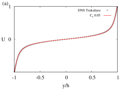
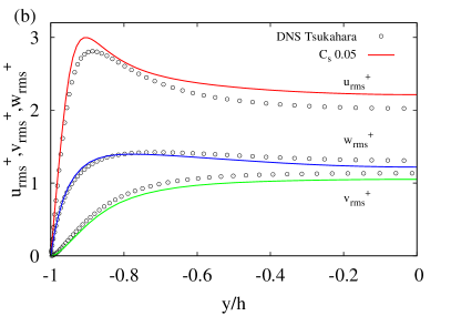
Figure 1: Comparison of the reference LES ($C_{s}=0.05$, lines) results obtained in the VLSM-Box  to the data (symbols) of Tsukahara et al. (2006) obtained by DNS in domains of similar extension at the same Reynolds number Re=2150 ($Re_{\tau}=128$). The mean flow profiles $U^{+}$ are compared in panel $a$ while in panel $b$ are reported the $rms$ velocity profiles $u^{\prime+}_{rms}$, $v^{\prime+}_{rms}$ and $w^{\prime+}_{rms}$.

The mean-velocity and $rms$ velocity profiles of the reference LES are in reasonably good agreement with the DNS data of Tsukahara et al. (2006), as shown in figure 1. In the instantaneous field visualised in figure 2$(a)$, very long streaky structures with the spanwise spacing roughly at $\lambda_{z}\approx 4h-5h$ are clearly visible throughout the entire domain on top of small-scale background turbulence, in agreement with previous simulations (see e.g. Komminaho et al., 1996; Tsukahara et al., 2006). The large-scale streaks also show the characteristic ‘ramp’ structure of the low-speed regions with angles $\approx 10^{o}-12$ to the wall (see figure 3) already observed e.g. in turbulent boundary layers (see e.g. figure 8 of Dennis & Nickels, 2011).

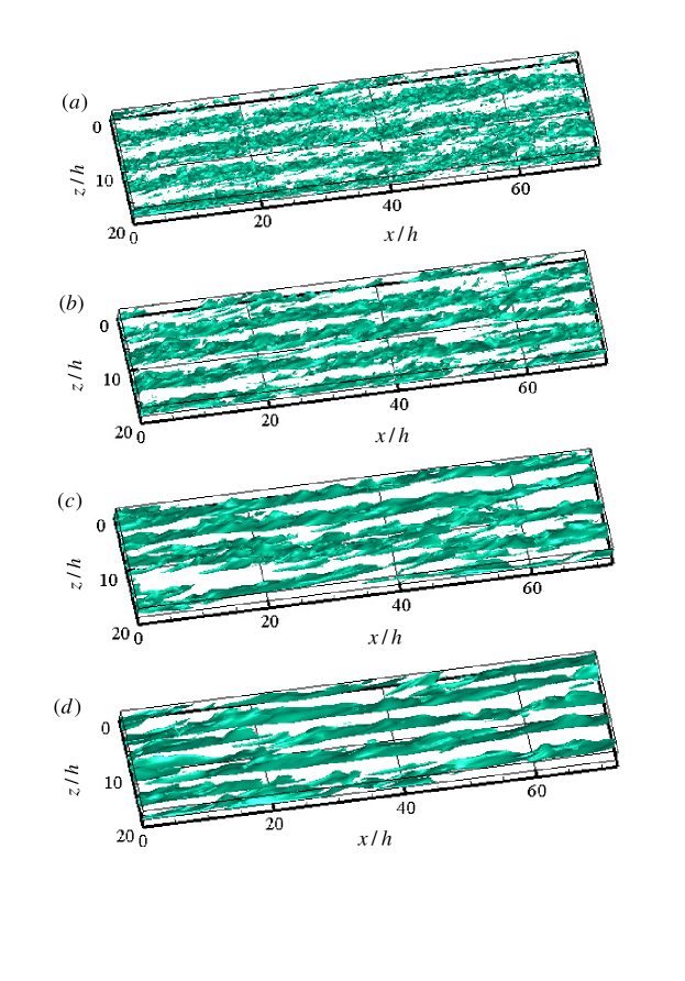
Figure 2: Iso-surface ($u^{+}=-2.5$) of the instantaneous negative streamwise velocity fluctuations (low speed streaks) on the lower wall at ${\rm Re}=2150$: (a) $C_{s}=0.05$ (reference case); (b) $C_{s}=0.10$; (c) $C_{s}=0.14$; (d) $C_{s}=0.18$. The visualization illustrates that the progressive quenching of small-scale motions for increasing values of $C_{s}$ does not affect the self-sustainment of large and very large-scale streaky motions.

One-dimensional spectra of the streamwise velocity shown in figure 4 are also in good agreement with the DNS ones reported by Tsukahara et al. (2006). The spanwise spectra reveal two well-separated peaks depending on the wall-normal location (figure 4$a$). The first peak appears at $\lambda_{z}^{+}\simeq 100$ in the near-wall region ($y^{+}\leq 30$), while the second peak is at $\lambda_{z}\approx 4h-5h$ in the outer region ($y\geq 0.2h$); the former corresponds to near-wall streaks whereas the latter corresponds to large and very-large scale streaky structures. The streamwise spectra have a peak at $\lambda_{x}^{+}\simeq 700$ in the near-wall region, which is representative of near-wall streaks. In the outer region, the spectra exhibit two peaks, one at $\lambda_{x}\approx 10h$ and the other at $\lambda_{x}\approx 42h-64h$. The two peaks at $\lambda_{x}\approx 10h$ and $\lambda_{x}\approx 42h-64h$, which are also in good agreement with the DNS results, correspond respectively to large (LSM) and very large-scale motions (VLSM).

A terminological note is necessary here. We choose to use the LSM and VLSM terminology also in Couette flow, where it does not appear to be currently standard, because we think that the mechanisms underlying their dynamics are common to other wall-bounded turbulent shear flows. Also, we will denote by VLSM only structures that have a very large (e.g. $\approx 40-60h$) but finite streamwise wavelength. These motions can be detected only in very long domains. Structures with infinite wavelength in the streamwise direction will not be referred to as VLSM because streamwise uniform motions can not self-sustain (see e.g. Waleffe, 1995) and therefore are not of interest here.

3.2 Overdamped simulations: self-sustained large-scale motions

Having validated the ability of the reference LES to quantitatively reproduce the main features of the turbulent Couette flow obtained by DNS in previous studies, we now examine if the motions at large scales persist even in the absence of smaller-scale active motions in the near-wall region. As in Hwang & Cossu (2010b), we therefore gradually increase the Smagorinsky constant $C_{s}$, which determines the filter width of the LES, to remove the small-scale active structures from the near-wall region. It should be noted that the increase of $C_{s}$ does not significantly affect the friction Reynolds number ${\rm Re}_{\tau}=128$ of the reference simulation ($C_{s}=0.05$): it is indeed found that ${\rm Re}_{\tau}=119$ for $C_{s}=0.10$, ${\rm Re}_{\tau}=117$ for $C_{s}=0.14$, ${\rm Re}_{\tau}=119$ for $C_{s}=0.18$.

The flow fields visualised in figure 2 show that the small-scale turbulent motions are gradually damped out as $C_{s}$ is increased. For $C_{s}=0.14$ (figure 2$d$), only the motions at large and very large scale are left in the flow field, suggesting the outer motions are likely to be sustained by themselves. The survival of the large-scale motions persist at $C_{s}=0.18$ (see figure 2$d$), although they are eventually quenched for $C_{s}=0.25$ (not shown). The examination of figure 3 further confirms that when small-scale motions are smoothed out the surviving coherent large and very-large scale structures are reasonably similar to the `natural' ones obtained in the reference case. In particular, they show the typical `ramp' structure of the low-speed regions with angles $\approx 10^{o}-12^{o}$ to the wall.

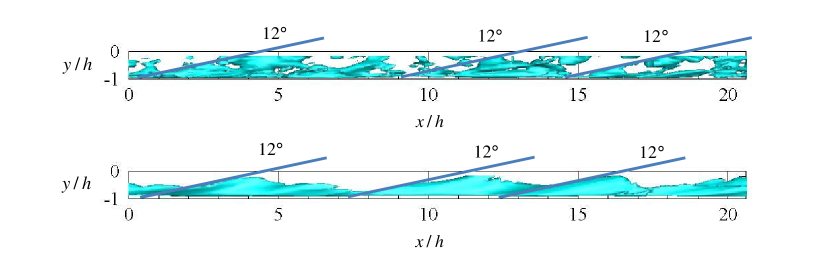
Figure 3: Side view of the low velocity fluctuations in the VLSM-Box  for the reference case $C_{s}=0.05$ (top panel) and the over-damped $C_{s}=0.14$ (bottom panel) at ${\rm Re}=2150$. The data are the same as in panels $a$ and $c$ of figure 2. In order to highlight the ramp structure of large-scale motions, only a limited streamwise part of the computational domain is represented and the levels $u^{+}=-3.9$ for $C_{s}=0.05$ and $u^{+}=-5.3$ for $C_{s}=0.14$ are used. The $12^{o}$ angle is measured from the wall.

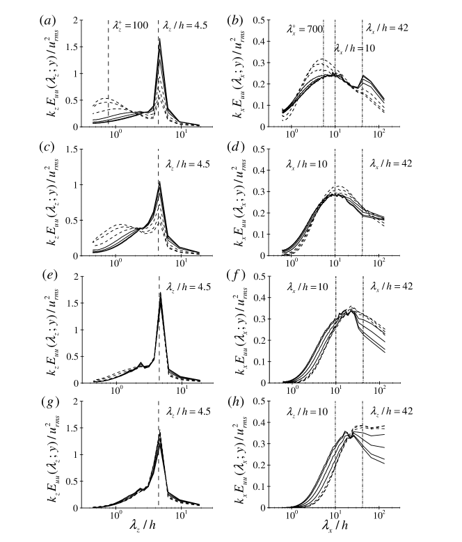
Figure 4: Spanwise premultiplied power spectra $k_{z}E_{uu}(\lambda_{z})$ [(a), (c), (e), (g)] and streamwise premultiplied power spectra $k_{x}E_{uu}(\lambda_{x})$ (panels $b$, $d$, $f$, and $h$) for respectively the reference simulation with $C_{s}=0.05$ (panels $a$ and $b$) and for the cases $C_{s}=0.10$ ($c$ and $d$) and $C_{s}=0.14$ ($e$ and $f$) and $C_{s}=0.18$ ($g$ and $h$). The premultiplied spectra are extracted in the inner- ($y^{+}=11,17,28$ based on $Re_{\tau}$ of the reference simulation, dashed lines) and in the outer layer (at distances from the bottom wall of $y+h=0.40h,0.57h,0.78h,h$ solid lines).

The premultiplied spectra reported in figure 4 provide a quantitative confirmation of this scenario. The original ($C_{s}=0.05$) peak location of the near-wall motions at $\lambda_{z}^{+}\simeq 100$ in the spanwise spectra (figure 4$a$) is initially shifted to a larger spanwise wavelength for $C_{s}=0.10$ (figure 4$c$) and completely suppressed for $C_{s}=0.14$ (figure 4$e$) and higher (figure 4$g$), where only the footprint of large-scale motions appears in the near wall region. Similar features are observed in the streamwise spectra where the original peak location at $\lambda_{x}^{+}\simeq 700$ in the near-wall region (figure 4$b$) is shifted to higher wavelengths up to its complete suppression (figure 4$d$, $f$ and $h$).

In contrast, large-scale motions (LSM) appear to be fairly robust to the increase of $C_{s}$. The peak at $\lambda_{z}\simeq 4.5h$ in the spanwise spectra robustly remains at the same location for all increasing values of $C_{s}$ (figure 4$a$, $c$, $d$ and $e$). In the streamwise spectra, for $C_{s}=0.10$ the LSM peak at $\lambda_{x}\simeq 10h$ remains unchanged, while the VLSM peak at $\lambda_{x}\simeq 42h-64h$ is blurred. For $C_{s}=0.14$, the original location of the first peak ($\lambda_{x}\simeq 10h$) has drifted to a slightly longer streamwise wavelength ($\lambda_{x}\simeq 14h$) (figure 4$f$), and it appears that this feature makes the presence of the VLSM structures even more blurred. Similar drifts of the streamwise wavelength of LSM for relatively large $C_{s}$ have also been observed in the case of the pressure-driven channel flow (Hwang & Cossu, 2010b). When $C_{s}=0.18$, the artificial over-damping begins to have a non-negligible effect on the dynamics of large-scale motions in the near-wall region where energy accumulates at the longest available streamwise wavelengths. This is why in figure 3 and in the following we only discuss the dynamics of structures corresponding to $C_{s}\lesssim 0.14$.

These results suggest that motions with typical spanwise spacings $\lambda_{z}\simeq 4h-5h$ sustain by a process which is not forced by motions at smaller scales. The relation between large-scale (LSM) and very-large scale motions (VLSM) is left partially unsolved by these simulations because they do not exclude that the self-sustained process is associated to the VSLM very long wavelengths. The reference and overdamped simulations have been therefore repeated in a smaller domain (the LSM-Box  listed in table 1) having the typical dimensions of large-scale motions. The results of this additional series of LES, discussed in appendix A, are very similar to the ones discussed above and show that large-scale motions self-sustain also in the absence of potentially active motions of even larger scale when near-wall active processes are quenched. There is therefore an active process at precisely this scale ($\lambda_{z}\approx 4h-5h$, $\lambda_{x}\approx 10h-12h$). The nature of this process is further explored in the next section.

4 Steady 'exact' nonlinear large-scale solutions of the filtered equations

The overdamped simulations of filtered motions have shown that large-scale motions can self-sustain even when near-wall motions are artificially quenched. Similarly to what has been done to understand transitional structures for the Navier-Stokes equations, we investigate the specific mechanism by which turbulent large-scale motions sustain by looking for the existence of nonlinear `exact' solutions. More specifically, we look for steady solutions of the filtered equations at Reynolds numbers where the flow is in a fully developed turbulent state. To make the steady state computations manageable and to avoid potentially active very-large scale motions to come into the picture we consider the domain LSM-Box-Newton listed in table 1, whose size $L_{x}\times L_{z}=10.9h\times 5.5h$ is that of large-scale motions (see figure 4). The dimensions of the LSM-Box  also correspond to those of the 'optimum' domain considered by Waleffe (2003) and are very similar to those of domains in which early `transitional' steady solutions of the (unfiltered) Navier-Stokes equations have been found (Nagata, 1990; Clever & Busse, 1992). We will show that this is not a mere coincidence, and that these solutions, that we will denote by NBCW (Nagata-Busse-Clever-Waleffe), are indeed much more related to self-sustained large-scale motions than to near-wall cycles.

4.1 Coherent steady solutions at Re=750

We begin by looking for exact solutions near the relatively low Reynolds number ${\rm Re}=750$ (corresponding to ${\rm Re}_{\tau}=52$), which roughly corresponds to twice the value of the transitional Reynolds number. The box discretization details are reported in table 1. It has been verified (Rawat, 2014) that reference large eddy simulations at the considered ${\rm Re}=750$ with $C_{s}=0.05$ in the LSM-Box compare well to the DNS results obtained in the same box and are relatively similar to those obtained in larger domains at the same Reynolds number (see also Komminaho et al., 1996; Tsukahara et al., 2006, for a discussion of the box size effects). The premultiplied spectra also show a reasonable agreement with the DNS results for $C_{s}=0.05$ and only large-scale motions survive when the near-wall cycle is artificially quenched by increasing the Smagorinsky constant $C_{s}$ (Rawat, 2014).

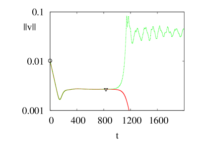
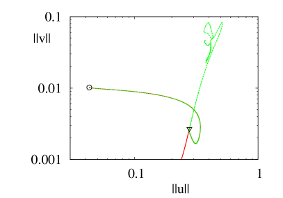
Figure 5: Edge tracking in the over-damped LES at Re=750 (${\rm Re}_{\tau}=52$) and $C_{s}=0.14$. Two initial conditions (circle symbol) lying almost on the edge of chaos surface initially remain near the surface while being attracted to the steady solution edge state (triangle symbol). The solution lying on the upper side of the edge of chaos (green line, dotted) finally evolves toward a state with irregular large-scale active motions while the other one (solid, red line) finally relaxes to a state with no large-scale active motions. The trajectories are shown in both the $t-\|v\|$ (top panel) and in the $\|u\|-\|v\|$ plane (bottom panel) displaying the streaks-vortices dynamics.

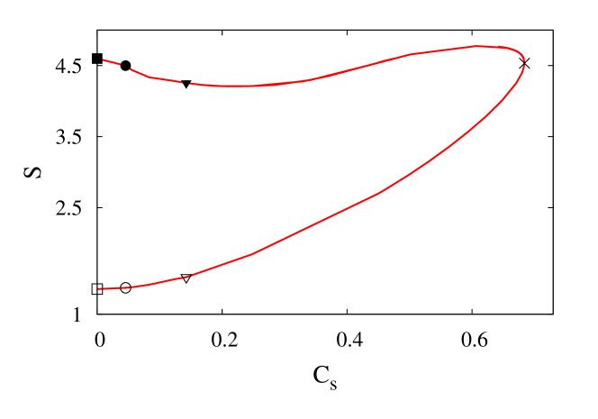
Figure 6: Continuation diagram of the steady solutions in the Smagorinsky constant $C_{s}$ at ${\rm Re}=750$ (${\rm Re}_{\tau}=52$). $S=\tau_{w}/(\mu U_{w}/h)$ is the wall shear rate of the solution normalized by its laminar value. The symbols denote the solutions found at $C_{s}=0$ (Navier-Stokes, squares, with $S=1.37$ on the lower branch and $S=4.59$ on the upper branch), $C_{s}=0.05$ (reference LES, circles) and $C_{s}=0.14$ (overdamped LES where the edge-tracking has been performed, triangles). Empty symbols denote lower branch solutions, filled symbols denote upper branch solutions.

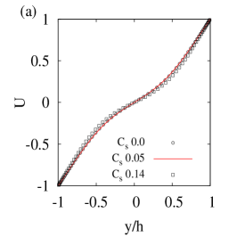
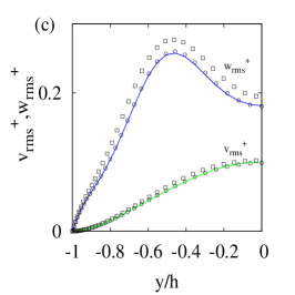
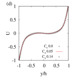
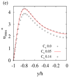
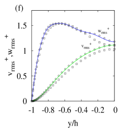
Figure 7: Lower (panels $a$, $b$ and $c$) and upper (panels $d$, $e$ and $f$) branch steady solutions in the LSM-Box at Re=750 (${\rm Re}_{\tau}=52$): mean flow (panels $a$ and $d$), streamwise (panels $b$ and $e$) and cross-stream (panels $c$ and $f$) $rms$ velocity profiles corresponding to $C_{s}=0.14$ (overdamped large eddy simulation), $C_{s}=0.05$ (reference large eddy simulation) and $C_{s}=0$ (Navier-Stokes steady solution).

As discussed in §2.2, an edge-tracking technique can be effective to compute lower-branch steady solutions in plane Couette flow. We therefore apply the edge-tracking technique to the overdamped LES simulations with $C_{s}=0.14$ at Re=750 in the LSM-Box  where the near-wall cycle is quenched and only large-scale motions survive. The initial condition given to the LES simulations consists in the mean turbulent flow to which is added a pair of streamwise-uniform counter-rotating rolls along with a sinuous perturbation of the spanwise velocity, which is similar to that used by Toh & Itano (2003) and Cossu et al. (2011): ${\mathbf{u}}_{0}=\left\{U(y),0,0\right\}+A_{0}\left\{0,\partial\psi_{0}/\partial z,-\partial\psi_{0}/\partial y\right\}+0.1\,A_{0}\left\{0,0,w_{sin}\right\}$ where $\psi_{0}(y,z)=\left(1-y^{2}\right)\,\sin\left(2\pi z/L_{z}\right)$ and $w_{sin}(x,y)=\left(1-y^{2}\right)\,\sin\left(2\pi x/L_{x}\right).$ The bisection is performed by adjusting the amplitude $A_{0}$ of the perturbations. The results of the edge tracking, displayed in figure 5, show that the edge state solution has constant energy. The initial transient clearly shows the coherent transient growth of the initial condition (slow decrease of the wall-normal velocity perturbations and high increase of the streamwise streaks norm $\|u\|$) leading to the edge state.

The edge-tracking solution is then used as an initial guess for Newton-Krylov iterations, performed with the peanuts  code. The solver converges to a steady solution (i.e. with zero phase speed, up to the precision of the Newton solver computation) of the (LES) equations for the filtered motions. The converged solution can be continued in $C_{s}$ using a Newton-based continuation. When continued to higher $C_{s}$, the solution encounters a saddle-node bifurcation from which the lower branch and an associated upper branch originate, as shown in figure 6. As the solutions obtained for $C_{s}\gtrsim 0.18$ lose much of their physical relevance because the LSM become themselves over-damped, the high-$C_{s}$ continuation should be considered only as a method (just as an homotopy) to access upper branch solutions. Also, it must be noted that the high-$C_{s}$ bifurcation is not simply reproducing the low-${\rm Re}$ bifurcation of Navier-Stokes solutions. Here the stress tensor depends non-linearly on the rate of strain, which models turbulent dissipation. As a consequence, e.g. the value of shear parameter $S$ at the the saddle-node bifurcation is more than the double of the value of $S$ at the low-Reynolds number saddle-node bifurcation of Navier-Stokes solutions.

Even more interestingly, both upper and lower branch solutions can be continued to lower values of $C_{s}$ and in particular to $C_{s}=0.05$, the `reference' value used to match DNS solutions, and even to $C_{s}=0$ which corresponds to solutions of the (unfiltered) Navier-Stokes equations. The mean and $rms$ velocity profiles corresponding to $C_{s}=0.14$, $C_{s}=0.05$ and $C_{s}=0$, reported in figure 7, are very similar to one another and do remind the NBCW solutions of the Navier-Stokes equations. For the lower-branch solutions, most of the energy is concentrated in the quasi-streamwise streaky motions (mainly $u_{rms}$ component) which are forced by low-amplitude quasi-streamwise vortices (mainly the $v_{rms}$ component) while for the upper-branch solutions, quasi-streamwise streaks and vortices have comparable energy.

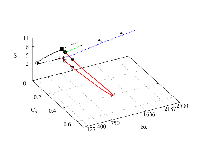
Figure 8: Continuation diagram of steady solutions in the $C_{s}-{\rm Re}$ parameters plane. The solid (red) line continuation in $C_{s}$ is that shown in figure 6 (see its caption for the meaning of the symbols). The continuation in Reynolds number at $C_{s}=0$ (black line, dashed) shows that the solutions continued from the turbulent case (square symbols) belong to the NBCW branch of Navier-Stokes solutions originating in a saddle-node bifurcation at ${\rm Re}=127$ (in this box with $L_{x}=10.89$ and $L_{z}=5.46$). It has been possible to directly continue the $C_{s}=0.05$ solution from ${\rm Re}=750$ to ${\rm Re}=1164$ (green line connecting to the solution denoted by a filled triangle). Nonlinear steady solutions at higher Reynolds numbers are found by first continuing the solutions obtained for $C_{s}=0.1$ to higher Re (blue line, dashed-dotted) and then reducing $C_{s}$ to $C_{s}=0.05$ (filled diamond symbols), except for the ${\rm Re}=2187$ solution which could only be continued to $C_{s}=0.06$.

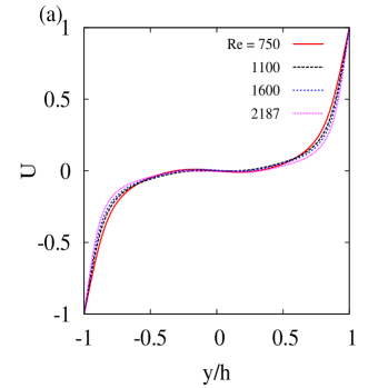
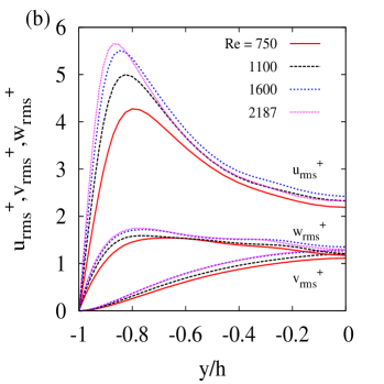
Figure 9: Mean flow (panel $a$) and $rms$ velocity profiles (panel $b$) corresponding to the upper branch coherent steady solutions obtained for increasing Reynolds numbers LSM-Box  ($C_{s}=0.06$ for ${\rm Re}=2150$ and $C_{s}=0.05$ otherwise).

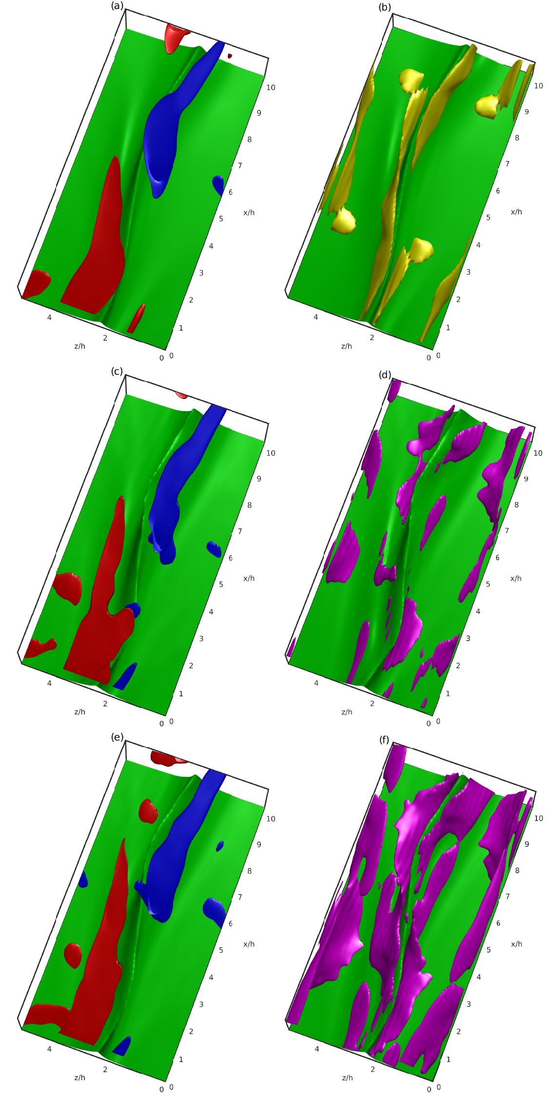
Figure 10: Visualisation of the upper branch large-scale coherent steady solutions of the LES equations obtained with the reference value $C_{s}=0.05$ and for increasing values of the Reynolds number: Re=750 (corresponding to ${\rm Re}_{\tau}=52$, top row), Re=1600 (${\rm Re}_{\tau}=99$, middle row), Re=2187 (${\rm Re}_{\tau}=127$, with $C_{s}=0.06$). The panels on the left represent the streaks and quasi-streamwise vortices: the green surface corresponds to a streamwise velocity value $50\%$ of its maximum value while the blue and green surfaces correspond streamwise vorticity values equal to $\pm 70\%$ of the maximum. The panels on the right represent the streaks and the relative eddy-viscosity associated to the filtered small-scale motions. The green surface is the same as in the left panel, while the violet surfaces correspond to $\nu_{t}/\nu=40\%$ and the yellow one to $\nu_{t}/\nu=10\%$.

4.2 Continuation to higher Reynolds numbers

The steady solutions obtained at ${\rm Re}=750$ are very similar to the NBCW solutions. We have therefore continued the solution corresponding to $C_{s}=0$ (i.e. the unfiltered Navier-Stokes solution) from ${\rm Re}=750$ to ${\rm Re}=400$ where it appears to be identical to the one computed by Waleffe (2003) in the same box at the same ${\rm Re}$. Continuation to lower ${\rm Re}$ indeed shows that the upper and the lower branch are connected by the saddle-node bifurcation at ${\rm Re}=127$ (Waleffe, 2003) as shown in figure 8.

At ${\rm Re}=750$ (${\rm Re}_{\tau}\approx 52$), the near-wall and large-scale motions scales are not yet separated enough to allow definitive conclusions on the nature of the steady solutions of the filtered equations. It is therefore potentially unclear that the computed steady solutions are associated to the self-sustained large-scale motions discussed in §3 and not to near-wall motions. In order to clarify this issue the coherent steady solutions of the over-damped LES have been continued to higher Reynolds numbers, keeping the box dimensions constants in outer units ($L_{z}=5.5h$ and $L_{x}=10.9h$).

We concentrate on upper branch solutions because they are most relevant to the turbulent dynamics (lower branch solutions are related to the transition problem which is probably less relevant in the turbulent regime). A continuation to higher ${\rm Re}$ fails to converge for Reynolds numbers larger than $Re\approx 1164$ (${\rm Re}_{\tau}\approx 74$) for the reference $C_{s}=0.05$ (but also for $C_{s}=0$). To circumvent this difficulty, an alternate path has been followed in the parameter space by first computing solutions at $C_{s}=0.1$, as shown in figure 8. The $C_{s}=0.1$ steady solutions can be continued up to $Re\approx 2500$. At selected Reynolds numbers ranging up to ${\rm Re}=2187$, the $C_{s}=0.1$ solutions can then be tracked down to $C_{s}=0.05$ except for ${\rm Re}=2187$, corresponding to ${\rm Re}_{\tau}\approx 127$, where the solution can not be continued below $C_{s}=0.06$.

The mean and $rms$ velocity profiles of the `reference' ($C_{s}=0.05$ and $C_{s}=0.06$ for the highest ${\rm Re}$) solutions obtained at these larger Reynolds numbers are reported in figure 9. The change of the wall-normal and spanwise $rms$ velocity profiles with the Reynolds number is minor. The peak streamwise $rms$ velocity, associated to the large-scale streaks, increases with the Reynolds number and is attained nearer to the wall. All the $rms$ velocity components remain relatively large in the bulk of the flow. These features are consistent with the observed behaviour of coherent large-scale motions (see e.g. Pirozzoli et al., 2014; Avsarkisov et al., 2014, for the most recent DNS results). This similarity is confirmed by the analysis of the flow fields associated to the large-scale coherent steady solutions reported in figure 10. This figure also illustrates how the eddy viscosity associated to the residual (small-scale) motions increases with the Reynolds number and is located mainly on the flanks of the low speed streak. The absolute levels of eddy viscosity are not huge even at ${\rm Re}=2187$ where the maximum of $\nu_{t}$ does not exceed $90\%$ of the molecular viscosity for those solutions but, contrary to the Navier-Stokes case, the eddy viscosity is not spatially uniform and depends on the local properties of the large-scale flow.

Having observed a clear relation between NBCW and coherent large-scale motions, it remains to verify if these solutions are also related to buffer-layer structures. This question is addressed in appendix B where it is shown that NBCW do not converge to buffer layer structures if continued to higher ${\rm Re}$ in minimal flow units with $L_{x}^{+}\times L_{z}^{+}=250\times 100$.

5 Summary and discussion

The main scope of this investigation has been to understand the origin of the coherent large-scale motions (LSM) which are numerically and experimentally observed in the turbulent plane Couette flow.

In the first part of the study, the self-sustained nature of large-scale motions has been investigated using the over-damped large eddy simulation technique introduced by Hwang & Cossu (2010b, 2011). The main results of the first part of the study can be summarized as follows:
(a) Reference large eddy simulations at ${\rm Re}=2150$ (corresponding to ${\rm Re}_{\tau}=128$) in the VLSM-Box  ($L_{x}\times L_{z}=132h\times 12.5h$) and with a sufficiently refined grid are able to capture the most important features of turbulent Couette flow, namely the near-wall cycle and the large and very large-scale motions (LSM & VLSM) with characteristics sizes in good agreement with those found in the direct numerical simulations of Tsukahara et al. (2006).
(b) Large-scale motions (LSM) do survive the quenching of the near-wall cycle at ${\rm Re}=2150$ with properties very similar to those of the `natural' large-scale motions.
(c) Large-scale motions also survive the quenching of the near-wall cycle in a `LSM-Box' with dimensions $L_{x}\times L_{z}=10.9h\times 5.5h$ typical of large-scale motions but where potentially active very-large scale motions of finite wavelength are excluded.

These results further confirm the findings of Hwang & Cossu (2010c) for the turbulent pressure-driven channel that a self-sustained process is at work at large scale in wall-bounded shear flows. The process is self-sustained because it does not rely on active motions at smaller or larger scales and its existence is in contrast with the current view that large-scale motions (LSM) ``are believed to be created by the vortex packets formed when multiple hairpin structures travel at the same convective velocity'' (as summarized in the review paper by Smits et al., 2011). Indeed, figures 2 and 3 clearly show that large-scale motions are still active even when the multiple smaller scale structures are removed from the scene. It must be noted that the LSM of the over-damped simulations can be only qualitatively similar to the real ones because the near-wall self-sustained process has been artificially shut down in order to prove that LSM are self-sustained. It is therefore almost surprising that the LSM of the over-damped simulations still reproduce so many features of the `real' ones despite the very strong modification of the flow induced by the over-damping.

In the second part of the study the nature of the self-sustained large-scale motions in turbulent Couette flow has been further investigated by looking for steady state solutions of the filtered equations (i.e. of the, possibly overdamped, LES) in a periodic domain with the typical dimensions of the LSM (the LSM-Box  with $L_{x}\times L_{z}=10.9h\times 5.5h$), which also coincide with those of the `optimum' domain considered by Waleffe (2003) for the transitional Couette flow. The main results can be summarized as follows:
(a) An upper and a lower branch of coherent large-scale steady solution of the filtered (LES) equations have been computed at ${\rm Re}=750$ by edge-tracking and using Newton iterations. These solutions have been continued in $C_{s}$ in the LSM-Box. The upper and lower branches are connected via a saddle-node bifurcation at high $C_{s}$.
(b) The continuation in $C_{s}$ also shows that both upper and lower branch solutions can be continued to the reference value $C_{s}=0.05$ and even to steady solutions of the Navier-Stokes equations obtained for $C_{s}=0$ up to ${\rm Re}=1164$.
(c) Coherent steady upper-branch solutions at the reference value $C_{s}=0.05$ have been computed at Reynolds numbers up to ${\rm Re}=2150$ using specific paths in the ${\rm Re}-C_{s}$ plane. The maximum amplitude of the associated large-scale streaks increases with the Reynolds number and its position approaches the wall on increasing ${\rm Re}$. The eddy viscosity associated with these solutions also increases with ${\rm Re}$.
(d) The solutions obtained for $C_{s}=0$ are shown to belong to the well known branch of NBCW solutions of the Navier-Stokes equations originating in a saddle-node bifurcation at ${\rm Re}=127$ (and $C_{s}=0$) in the LSM-Box.
(e) The continuation of the NBCW upper branch solutions to high Reynolds numbers in a minimal flow unit ($L_{x}^{+}\times L_{z}^{+}=250\times 100$) does not converge to solutions consistent with typical buffer-layer structures, as shown in appendix B.

This is, to the best of our knowledge, the first time that invariant `exact' solutions are computed for large-scale turbulent filtered, i.e. truly coherent, motions. These `exact' solutions of the LES equations, contrary to solutions of the Navier-Stokes equations take into account the effect of small scales only through their averaged effect. The spatial and Reynolds number dependence of the eddy viscosity associated with the averaged (residual) small-scale motions is naturally embedded in the computed solutions. It is, in this way, possible to compute coherent large-scale steady solutions despite the fact that motions at smaller scale are unsteady and therefore concentrate on the interesting dynamics of the large-scale coherent solutions without the less relevant complications associated to motions at smaller scales.

The features of the computed coherent steady state upper branch solutions are consistent with previous findings. For instance, the fact that the maximum streak amplitude associated with these large-scale solutions increases with the Reynolds number is consistent with the fact that the large-scale peak in premultiplied spectra of turbulent wall-bounded flows also increases with Reynolds number (e.g. Pirozzoli et al., 2014). It is also consistent with the fact that the maximum energy amplification of the most amplified streaks increases with the Reynolds number as predicted by the theoretical analyses of Pujals et al. (2009), Cossu et al. (2009), Hwang & Cossu (2010a, b) and Willis et al. (2010). That the position of the maximum streak amplitude approaches the wall for increasing ${\rm Re}$ is also in agreement with previous findings (see e.g. Mathis et al., 2011).

Another interesting result is that the coherent large-scale solutions are connected to the NBCW solutions of the Navier-Stokes equations and are relatively similar to them when continued to higher Reynolds numbers in the LSM-Box  whose dimensions remain constant in outer units. In previous studies the dynamics of NBCW solutions has been discussed for low Reynolds numbers where the spanwise size of large-scale and buffer-layer streaks are very similar. This ambiguity is removed here by considering sufficiently large Reynolds numbers where scale separation sets in between inner and outer layer structures and by showing that the NBCW solutions do not converge to typical buffer-layer structures when continued to higher ${\rm Re}$ in a minimal flow unit. NBCW solutions can therefore be considered as the `precursors' of large-scale motions.

This study is a second step, after that of Hwang & Cossu (2010c, 2011), towards a `dynamical systems' understanding of the large-scale dynamics in fully developed turbulent shear flows. The key ingredient is to model small-scale motions and to only resolve large-scale motions in order to compute invariant solutions. Much work remains to be done to assess the relevance of coherent invariant solutions of the filtered equations to the prediction of turbulent flow dynamics. Interesting questions left for future work are, for instance, to understand if other steady or periodic solutions of the LES equations can be computed and to know how much time turbulent solutions of large-eddy simulations spend in the neighbourhood of exact coherent large-scale solutions (in the same spirit of the Navier-Stokes computations of Kerswell & Tutty, 2007; Schneider et al., 2007). One could indeed hope that the increase in effective viscosity in fully developed turbulent large-scale flows, could lead to a `simpler' dynamics of large-scale motions where a few invariant solutions are sufficient to capture essential features of the flow as in the case of transitional flows (see e.g. Kawahara & Kida, 2001).

As the static Smagorinsky model used in this work is very crude, there certainly is room for improvement in the modelling of small-scale dynamics to compute self-sustained large-scale coherent motions more accurately. However, we believe that meaningful results can be found in other canonical wall-bounded shear flows using this over-damped LES technique even in its relatively primitive current form. The methods used in this study could also help to shed light on different problems involving shear flows, as for instance the very large Reynolds and/or magnetic Reynolds number behaviour of self-sustained processes in Keplerian shear flow (Rincon et al., 2007a, b, 2008; Herault et al., 2011; Riols et al., 2013), with possible practical applications to the modelling of the dynamics of astrophysical accretion disks (Riols et al., 2015).

Appendix A Reference and overdamped LES in the LSM-BOX

A series of simulations have been performed in the LSM-Box  with dimensions $L_{x}\times L_{z}=10.9h\times 5.5h$ typical of large-scale motions in order to verify if these motions can self-sustain in the absence of the potentially active very-large scale motions that were captured in the VLSM-Box discussed in §3. The number of grid points used in this box (see table 1) is chosen so as to keep the same grid spacing as in the VLSM-Box. Results are obtained at the same Reynolds number (${\rm Re}=2150$, corresponding to ${\rm Re}_{\tau}=128$) and for the same values of $C_{s}$ considered in §3 for the VLSM-Box. The spanwise and streamwise premultiplied spectra of the streamwise velocity component are shown in figure 11, which is the analogue of figure 4 of §3.

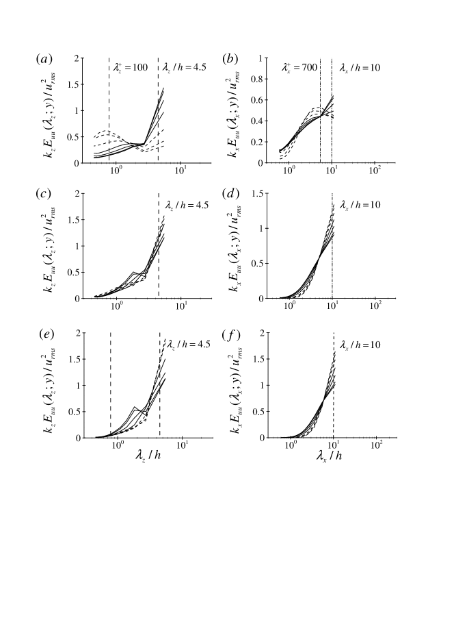
Figure 11: Premultiplied one-dimensional spanwise $(a,c,e)$ and streamwise $(b,d,f)$ spectra of the streamwise velocity in the LSM-Box  obtained for increasing values of the Smagorinsky constant: $(a,b)$ $C_{s}=0.05$ (reference value); $(c,d)$ $C_{s}=0.14$; $(e,f)$ $C_{s}=0.18$.

For the Reynolds number considered, the LSM-Box  (whose dimensions in inner units are $L_{x}^{+}\times L_{z}^{+}=1395\times 678$) is large enough to accommodate many near-wall structures. Indeed, at the reference value $C_{s}=0.05$, the near-wall peaks at $\lambda_{z}^{+}\simeq 100$ and at $\lambda_{x}^{+}\simeq 700$ are clearly visible in the spanwise and the streamwise spectra, respectively reported in figures 11$a$ and 11$b$. The spectral energy associated with the outer structures appears to be highly concentrated at the largest wavelengths allowed in the given computational domain which correspond to large-scale motions (LSM). As already mentioned, very-large scale motions (of finite streamwise wavelength) are out of the picture in the LSM-Box. On increasing $C_{s}$, the near-wall peaks are gradually quenched as in the spectra obtained in the VLSM-Box  (see figure 4). The outer structures in the confined domain appear to be well isolated at $C_{s}=0.14$ (figures 11$c$ and $d$) and persist even for the further increase of $C_{s}$ (figures 11$e$ and $f$). These results definitely confirm that the large-scale motions (LSM) are self-sustained in the absence not only of near-wall active processes but also in the absence of potentially active very-large scale motions (VLSM) of finite wavelength.

Appendix B Continuation of the NBCW solutions in a MFU

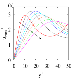
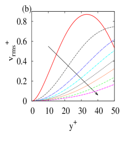
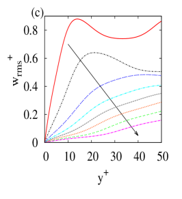
Figure 12: $rms$ velocity profiles of the nonlinear steady solutions obtained by continuation to higher Reynolds numbers of the NBCW solutions in minimal flow units with $L_{x}^{+}=250$ and $L_{z}^{+}=100$. The data corresponds to ${\rm Re}=400,750,1100,1200,\ldots,1500,1600$, with arrows indicating the increase in Reynolds number.

In this appendix we investigate if NBCW solutions can be continued into near-wall structures when the Reynolds number is sufficiently increased in minimal flow units (MFU). This issue is addressed in the case of the Navier-Stokes equations ($C_{s}=0$).

The main characteristic of the near-wall streaky structures is that their typical spanwise and streamwise lengths decrease when the Reynolds number is increased, but remain constant when expressed in wall units. Continuation of these solutions to higher Reynolds numbers should therefore be made keeping the box dimension fixed in wall units. As $L_{z}^{+}={\rm Re}_{\tau}L_{z}/h$, when ${\rm Re}_{\tau}$ is increased, $L_{z}$ must be decreased in order to keep constant $L_{z}^{+}$, and similarly for $L_{x}$. The approximate relation ${\rm Re}_{\tau}\approx 0.054\,{\rm Re}+11.22$ which fits well the data of a series of direct numerical simulations performed in the LSM-Box for ${\rm Re}\in[400,2150]$, is used to determine the box size. Attention must be paid to the grid resolution in the wall-normal direction because the size of the buffer-layer region, where near-wall streaks reside, also decreases when the Reynolds number is increased. In order to achieve a sufficient accuracy in the wall-normal direction, keeping the state vector size manageable for the Newton iterations, the time integrations required to perform the computation of the nonlinear solutions presented here have been performed using the channelflow code Gibson et al. (2008) which uses a Chebyshev spectral discretization in $y$, instead of the second-order finite difference discretization of diablo. This code can be used here because we do not consider large eddy simulations in this appendix. For these computations we use $N_{x}\times N_{y}\times N_{z}=32\times 65\times 32$ points. We have verified that the results do not change in any noticeable way when the number of points in the wall-normal direction is increased to $N_{y}=95$ for the highest considered Reynolds numbers.

The NBCW upper branch solution at ${\rm Re}=400$ is used as a starting point of the continuation. At ${\rm Re}=400$ the size of the LSM-Box, in inner units, is $L_{z}^{+}\approx 180$ and $L_{x}^{+}\approx 360$. As a preliminary step, this solution is continued in the parameters $L_{x}$ and $L_{z}$ to achieve $L_{z}^{+}\approx 100$ and $L_{x}^{+}\approx 200$ (which in external units corresponds to $L_{z}=2.6h$ and $L_{x}=5.51h$ (see also Gibson et al., 2008)). This steady solution is then continued by increasing the Reynolds number in small steps, changing the box size so as to keep it constant in inner units to $L_{z}^{+}=100$ and $L_{x}^{+}=250$ and predicting the initial guess on the velocity fields expressed in inner units. The Newton-based iterations are performed using peanuts.

The velocity profiles of the converged solutions are reported in figure 12 for selected Reynolds numbers and they appear to always belong to the same branch. The results show that the solutions continued in the near-wall minimal flow unit do not converge to near-wall structures. For instance, the $y^{+}$ position of the maximum of the $rms$ velocity profiles increases when ${\rm Re}_{\tau}$ is increased, while it should instead remain constant, as found by Jiménez & Moin (1991), in minimum flow unit simulations (see also Hwang, 2013). The NBCW solutions do not therefore seem to be connected to near-wall structures, at least in plane Couette flow, even if continued in minimal flow units, i.e. periodic domains which remain constant in inner units while increasing the Reynolds number.