Minimizing Dispersive Errors in Smoothed Particle Magnetohydrodynamics for Strongly Magnetized Medium

Abstract

In this study, we investigate the dispersive properties of smoothed particle magnetohydrodynamics (SPM) in a strongly magnetized medium by using linear analysis. In modern SPM, a correction term proportional to the divergence of the magnetic fields is subtracted from the equation of motion to avoid a numerical instability arising in a strongly magnetized medium. From the linear analysis, it is found that SPM with the correction term suffer from significant dispersive errors, especially for slow waves propagating along magnetic fields. The phase velocity for all wave numbers is significantly larger than the exact solution and has a peak at a finite wavenumber. These excessively large dispersive errors occur because magnetic fields contribute an unphysical repulsive force along magnetic fields. The dispersive errors cannot be reduced, even with a larger smoothing length and smoother kernel functions such as the Gaussian or quintic spline kernels. We perform the linear analysis for this problem and find that the dispersive errors can be removed completely while keeping SPM stable if the correction term is reduced by half. These findings are confirmed by several simple numerical experiments.

1 Introduction

Smoothed particle hydrodynamics (SPH) is an entirely Lagrangian particle method for simulating fluid flows [1, 2]. This Lagrangian nature offers major advantages when SPH is applied to problems with a large, dynamic range of spatial scales. Furthermore, SPH can easily incorporate other physics such as self-gravity, radiative transfer, or chemistry. Thus, SPH is widely used in a variety of astrophysical problems such as formation of large-scale structures, galaxies, stars, and planets.

Recently, several authors have tried to extend SPH to magnetohydrodynamics (MHD) because magnetic fields play an important role in a variety of astrophysical environments. In this study, we call SPH for MHD “smoothed particle magnetohydrodynamics” (SPM). Price and Monaghan [3] has developed an SPM method with artificial viscosity and resistivity [also see 4]. Iwasaki and Inutsuka [5] have applied Godunov’s method to SPM. We call it “GSPM”. Recently, Iwasaki and Inutsuka [6] have modified their original GSPM formulation, based on their derivation of the equation of motion in GSPM from an action principle.

Unfortunately, conservative formulations of SPM are known to inevitably suffer from numerical instability for low $\beta$ plasma because of negative stress, where $\beta$ is the ratio of the gas pressure to the magnetic pressure. This instability has already been pointed out by Phillips and Monaghan [7] [also see 8]. Among several methods proposed for removing the numerical instability [7, 8, 3], an approach by Børve, Omang, and Trulsen [9] is widely used in modern SPM methods [e.g., 4, 5, 6, 10]. A broad discussion of stable SPM schemes is found in a review by Price [11]. In the approach of Børve, Omang, and Trulsen [9], a correction term, ${\bf B}({\bf\nabla}\cdot{\bf B})/4\pi$, is subtracted from the right-hand side of the equation of motion. The correction term is essentially zero if ${\bf\nabla}\cdot{\bf B}=0$ is satisfied. By a linear analysis of SPM, Børve, Omang, and Trulsen [12] (hereafter BOT04) found that half of the correction term, or ${\bf B}({\bf\nabla}\cdot{\bf B})/8\pi$, is large enough to remove the numerical instability. This was confirmed by Barnes, Kawata, and Wu [13], who found that half the correction term provided the least error and minimized the violation of energy and momentum conservation in a variety of test calculations. Børve, Omang, and Trulsen [14] have proposed a sophisticated method, wherein the size of the correction term varies among the SPH particles.

However, it is still unclear how the correction term affects the capability of SPM to accurately model fluid flows. Guiding the optimal selection of the amount of correction in a rigorous manner is important. Balsara [15] have investigated the linear stability of various SPH formulations, kernel functions, and ratios of smoothing length to interparticle distance [also see 8, 16]. They have suggested an optimal range of parameters from obtained dispersion relations. Although these analyses are valid only for the linear regime and a regular particle configuration, they provide us with a lot of knowledge for achieving further improvements to SPM schemes. Pioneering work for SPM has been done by BOT04, who investigate the dispersive properties of SPM. They parameterize the size of the correction term with a free parameter $\xi$ $(0\leq\xi\leq 1)$, and use $\xi\times{\bf B}{\bf\nabla}\cdot{\bf B}/4\pi$ as the correction term. They found that as mentioned above, $\xi=1/2$ is large enough to stabilize SPM for low $\beta$ plasma, and also suggested that smoother kernels, such as Gaussian or the quintic spline kernels, reproduce correct phase velocities, while the cubic spline causes large dispersion errors. However, their study is restricted to several linear waves in the long-wavelength limit and to the case with $\xi=1/2$ although many authors still adopt $\xi=1$.

In this study, we investigate detailed dispersive properties of SPM for low $\beta$ plasma by changing $\xi$, the kernel functions, and the ratio of smoothing length to interparticle distance. From the results, a suggestion of an optimal choice of the size of the correction term is provided.

The paper is organized as follows: in Section 2, the basic equations of SPM are reviewed. In Section 3, a dispersion relation is derived from the basic equations of SPM and its asymptotic behavior in the long- and short-wavelength limits is discussed. The results of the linear analysis are presented in Section 4. To confirm the results of the linear analysis, several numerical experiments are demonstrated in Section 5. Our results are discussed in Section 6. Section 7 offers a summary.

2 SPM Equations

The basic equations of MHD are given by

$$\frac{\partial\rho}{\partial t}+{\bf\nabla}\cdot\left(\rho{\bf v}\right)=0,$$ (1)

$$\frac{\partial v^{\mu}}{\partial t}=\frac{1}{\rho}\nabla^{\nu}T^{\mu\nu}-\frac{\xi}{4\pi\rho}B^{\mu}\nabla^{\nu}B^{\nu},$$ (2)

and

$$\frac{d}{dt}\left(\frac{B^{\mu}}{\rho}\right)=\frac{B^{\nu}}{\rho}\nabla^{\nu}v^{\mu},$$ (3)

where $T^{\mu\nu}$ is the stress tensor,

$$T^{\mu\nu}=-\left(P+\frac{{\bf B}^{2}}{8\pi}\right)\delta^{\mu\nu}+\frac{B^{\mu}B^{\nu}}{4\pi},$$ (4)

and $d/dt=\partial/\partial t+{\bf v}\cdot{\bf\nabla}$ is the Lagrangian time derivative. The second term on the right-hand side of equation (2) is the correction term introduced to remove the numerical instability (BOT04). The parameter $\xi$ specifies the size of the correction term. In this study, $\xi$ is assumed to be constant for all particles. For simplicity, instead of the energy equation, the isothermal equation of state is assumed:

$$P=c^{2}\rho,$$ (5)

where $c$ is the sound speed. In the adiabatic case, the dispersive properties of SPM are expected to be qualitatively the same as those in the isothermal case.

In SPH, the density of the $a$-th particle is evaluated by the following equation:

$$\rho_{a}=\sum_{b}m_{b}W({\bf x}_{a}-{\bf x}_{b},h),$$ (6)

where the subscripts denote the particle label, $m_{b}$ is the mass of the $b$-th particle, $W({\bf x},h)$ is a kernel function, and $h$ is the smoothing length. In the linear analysis presented in this study, the smoothing length is assumed to be constant. In the numerical experiments shown in Section 5, a variable smoothing length is used.

There are several conservative formulations of SPM. Here, we show two schemes: the standard SPM formulation, the GSPM formulation. The basic equations of standard SPM [9, 3, 4] are given by

$$\frac{dv_{a}^{\mu}}{dt} = \sum_{b}m_{b}\left(\frac{T_{a}^{\mu\nu}}{\Omega_{a}\rho_{a}^{2}}\nabla_{a}^{\nu}W_{ab}(h_{a})+\frac{T_{b}^{\mu\nu}}{\Omega_{b}\rho_{b}^{2}}\nabla_{a}^{\nu}W_{ab}(h_{b})\right)$$ (7)

$$- \xi\frac{B_{a}^{\mu}}{4\pi}\sum_{b}m_{b}\left(\frac{B_{a}^{\nu}}{\Omega_{a}\rho_{a}^{2}}\nabla_{a}^{\nu}W_{ab}(h_{a})+\frac{B_{b}^{\nu}}{\Omega_{b}\rho_{b}^{2}}\nabla_{a}^{\nu}W_{ab}(h_{a})\right)+\left(\frac{dv^{\mu}}{dt}\right)_{\mathrm{diss}},$$

and

$$\frac{d}{dt}\left(\frac{B^{\mu}}{\rho}\right)_{a}=\frac{B_{a}^{\nu}}{\Omega_{b}\rho_{a}^{2}}\sum_{b}m_{b}\left(v_{a}^{\mu}-v_{b}^{\mu}\right)\nabla_{a}^{\nu}W_{ab}(h_{a})+\left[\frac{d}{dt}\left(\frac{B^{\mu}}{\rho}\right)_{a}\right]_{\mathrm{diss}},$$ (8)

where $W_{ab}(h_{a})=W({\bf x}_{a}-{\bf x}_{b},h_{a})$, the artificial dissipation terms (viscosity and resistivity) are denoted by the subscript of “diss”, and $\Omega$ denotes the effect of the variation of the smoothing length. The detailed expression is described in Price and Monaghan [3].

Iwasaki and Inutsuka [5, 6] implemented GSPM given by

$$\frac{dv_{a}^{\mu}}{dt} = \sum_{b}m_{b}\left(\frac{\left(T_{a}^{\mu\nu}\right)^{*}}{\Omega_{a}\rho_{a}^{2}}\nabla_{a}^{\nu}W_{ab}(h_{a})+\frac{\left(T_{b}^{\mu\nu}\right)^{*}}{\Omega_{b}\rho_{b}^{2}}\nabla_{a}^{\nu}W_{ab}(h_{b})\right)$$ (9)

$$- \xi\frac{B_{a}^{\mu}}{4\pi}\sum_{b}m_{b}\left(\frac{B_{a}^{\nu}}{\Omega_{a}\rho_{a}^{2}}\nabla_{a}^{\nu}W_{ab}(h_{a})+\frac{B_{b}^{\nu}}{\Omega_{b}\rho_{b}^{2}}\nabla_{a}^{\nu}W_{ab}(h_{a})\right),$$

in which the quantities with the asterisks are the results of a Riemann solver. The evolution equation of $B^{\mu}/\rho$ is the same as that of standard SPM, except for the artificial resistivity term. In Iwasaki and Inutsuka [6], the resistivity term is derived from the method of characteristics for Alfvén waves [17]. Note that equations (9) is a simplified version of a rigorous expression which is found in Iwasaki and Inutsuka [5, 6].

Balsara [15] and Morris [8, 16] have shown that the choice of kernel functions significantly influences on dispersive properties of SPH, and should be determined by the requirements of accuracy and computational efficiency. We consider several kernel functions to investigate how they affect the dispersive properties of SPM. The first is the Gaussian kernel, which has the best interpolation accuracy. It is given by

$$W_{\mathrm{G}}(r,h)=\left(\frac{1}{\sqrt{\pi}h}\right)^{d}e^{-(r/h)^{2}},$$ (10)

where $d$ is the number of dimensions. One disadvantage of the Gaussian kernel is its infinite extent; in actual calculations, the contributions for $r>3.1h$ are ignored. Also, in the linear analysis, we use a truncated Gaussian kernel at $r=3.1h$ that is denoted by $W_{\mathrm{tG}}$. Most works use the cubic spline kernel [18, 19], which is given by

$$W_{\mathrm{4}}(r,h)=\frac{C_{d}}{h^{d}}\left\{\begin{array}[]{ll}1-\frac{3}{2}s^{2}+\frac{3}{4}s^{3}&\;\;\mathrm{for}\;\;0\leq s\leq 1\\ \left(2-s\right)^{3}/4&\;\;\mathrm{for}\;\;1<s\leq 2\\ 0&\;\;\mathrm{otherwise}\end{array}\right.,$$ (11)

where $s=r/h$, and $C_{1}=2/3$, $C_{2}=10/7\pi$, and $C_{3}=1/\pi$. This kernel has a great computational advantage, as it has a compact support at $r=2h$. However, the interpolation is inaccurate and leads to relatively large dispersion errors in sound waves [15]. We also consider the quintic spline kernel,

$$W_{\mathrm{6}}(r,h)=\frac{C_{d}}{h^{d}}\left\{\begin{array}[]{ll}-10s^{5}+30s^{4}-60s^{2}+66&\;\;\mathrm{for}\;\;0\leq s\leq 1\\ 5s^{5}-45s^{4}+150s^{3}-120s^{2}+75s+51&\;\;\mathrm{for}\;\;1<s\leq 2\\ -s^{5}+15s^{4}-90s^{3}+270s^{2}-405s+243&\;\;\mathrm{for}\;\;2<s\leq 3\\ 0&\;\;\mathrm{otherwise}\end{array}\right.,$$ (12)

where $C_{1}=1/120$, $C_{2}=7/478\pi$, and $C_{3}=1/120\pi$. This kernel is smoother and more accurate kernel than $W_{4}$.

3 Linear Analysis

A two-dimensional (2D) rectangular lattice of particles with an interval of $\Delta x$ is considered as an unperturbed state. The position of the $a$-th particle position is given by ${\bf x}_{a0}=(\Delta x){\bf a}$, where ${\bf a}$ is the 2D integer vector, ${\bf a}=(a_{x},a_{y})$ ($a_{x},a_{y}=0,1,2,\cdots$). The particle mass $m_{0}$ and smoothing length $h$ are assumed to be constant. The following perturbations are considered:

$${\bf x}_{a}={\bf x}_{a0}+\delta{\bf x}_{a}$$ (13)

$$\rho_{a}=\rho_{0}+\delta\rho_{a}$$ (14)

$${\bf v}_{a}=\delta{\bf v}_{a}$$ (15)

$${\bf B}_{a}={\bf B}_{0}+\delta{\bf B}_{a}$$ (16)

$$P_{a}=P_{0}+c^{2}\delta\rho_{a},$$ (17)

where the subscript “0” indicates physical variables in the unperturbed state. For simplicity, the unperturbed magnetic field is assumed to be parallel to the $x$-direction, and fluctuations in the $z$-direction that correspond to Alfvén wave are not considered, although their propagation can be partly investigated by fast waves propagating along magnetic fields for low $\beta$ plasma. This means that we consider fast and slow modes that oscillate in the $(x,y)$-plane. We assume that the perturbations have the following space and time dependence:

$$\delta Q_{a}\propto\exp\left\{i\left({\bf k}\cdot{\bf x}_{a0}-\omega t\right)\right\},$$ (18)

where $\delta Q_{a}=(\delta{\bf x}_{a},\delta\rho_{a},\delta{\bf v}_{a},\delta{\bf B}_{a})$.

Substituting equations (13)-(17) into the standard SPM equations (6), (7), (8), and $d{\bf x}_{a}/dt={\bf v}_{a}$, we obtain a dispersion relation. The artificial dissipation term is omitted in this analysis. We do not repeat the detailed derivation of the dispersion relation that was already shown by BOT04. The dispersion relation is given by

$$\mathrm{det}\left(\omega^{2}\delta^{\mu\nu}+A^{\mu\nu}\right)=0$$ (19)

where “det” indicates determinant,

$$A^{\mu\nu}=\frac{2T_{0}^{\mu\eta}}{\rho_{0}}\left(\Psi^{\eta\nu}-\phi^{\eta}\psi^{\nu}\right)-\frac{1}{\rho_{0}}\left\{P_{0}\phi^{\mu}\psi^{\nu}+\frac{1}{4\pi}\left({\bf B}_{0}^{2}\delta^{\mu\nu}-B_{0}^{\mu}B_{0}^{\nu}\right){\phi}^{\zeta}{\psi^{\zeta}}\right\},$$ (20)

$T_{0}^{\mu\nu}$ is the unperturbed stress tensor modified by the correction term,

$$T_{0}^{\mu\nu}=-\left(P_{0}+\frac{{\bf B}_{0}^{2}}{8\pi}\right)\delta^{\mu\nu}+\left(1-\xi\right)\frac{B_{0}^{\mu}B_{0}^{\nu}}{4\pi},$$ (21)

$\psi^{\mu}$, $\phi^{\mu}$, and $\Psi^{\mu\nu}$ are given by

$$\psi^{\mu}=\sum_{b}\frac{m_{0}}{\rho_{0}}\left(1-e^{-i{\bf k}\cdot\left({\bf x}_{a0}-{\bf x}_{b0}\right)}\right)\frac{\partial W_{ab,0}}{\partial x_{a0}^{\mu}},$$ (22)

$$\phi^{\mu}=\sum_{b}\frac{m_{0}}{\rho_{0}}\left(1+e^{-i{\bf k}\cdot\left({\bf x}_{a0}-{\bf x}_{b0}\right)}\right)\frac{\partial W_{ab,0}}{\partial x_{a0}^{\mu}},$$ (23)

and

$$\Psi^{\mu\nu}=\sum_{b}\frac{m_{0}}{\rho_{0}}\left(1-e^{-i{\bf k}\cdot\left({\bf x}_{a0}-{\bf x}_{b0}\right)}\right)\frac{\partial^{2}W_{ab,0}}{\partial x_{a0}^{\mu}\partial x_{a0}^{\nu}}.$$ (24)

The first term on the right-hand side of equation (20) comes from the perturbation of $(1/\rho_{a}^{2}+1/\rho_{b}^{2})\nabla^{\nu}W_{ab}$, and the second term comes from the perturbation of $T^{\mu\nu}$ in equation (7).

Note that the dispersion relation derived from the linearized GSPM equations is identical to equation (19) if the physical quantities with an asterisk are evaluated at the arithmetic mean between the $a$- and $b$-th particles. Thus, this linear analysis is valid both in standard SPM and GSPM.

Since equation (19) is a quadratic equation in terms of $\omega^{2}$, two modes are obtained. In this study, the mode with larger (smaller) $\omega^{2}$ is referred to as the fast (slow) mode. The numerical phase velocities $\omega/|{\bf k}|$ of the fast and slow modes are denoted by $c_{\mathrm{f,num}}({\bf k})$ and $c_{\mathrm{s,num}}({\bf k})$, respectively.

3.1 Asymptotic behaviors

In this section, we investigate the asymptotic behavior of the dispersion relation in the short- and long-wavelength limits.

3.1.1 Short-wavelength Limit

SPM without the correction term is unstable for low $\beta$ plasma because negative diagonal components appear in the stress tensor [8]. The development of numerical instability begins with the growth of fluctuations whose scales are comparable to $\Delta x$. Thus, in this section, we investigate the asymptotic behavior in the short-wavelength limit and the size of $\xi$ required to stabilize SPM. Note that this already has been done by BOT04, who numerically solve the dispersion relation. Here, we show that their conclusion is reproduced in the following simple analytical manner.

In the discrete system, the largest wavenumber is $k=\pi/\Delta x$ where the unit wavelength is expressed by two particles. A compressible wave propagating along ${\bf B}_{0}$ (${\bf k}=(\pi/\Delta x,0)$) is considered. This corresponds to the slow mode. In this case, we obtain $\phi^{\mu}=\psi^{\mu}=0$ from equations (22) and (23). From equation (19), the dispersion relation becomes

$$\omega^{2}=-A^{xx}=\frac{2P_{0}}{\rho_{0}}\left(1-\frac{1-2\xi}{\beta}\right)\sum_{b}\frac{m_{0}}{\rho_{0}}\left(1-\left(-1\right)^{a_{x}-b_{x}}\right)\frac{\partial^{2}W_{ab,0}}{\partial x_{a0}^{2}},$$ (25)

where $\beta\equiv 8\pi P_{0}/B_{0}^{2}$. The summation in equation (25) is positive in normal situations [8]. Without the correction term ($\xi=0$), one can see that SPM becomes unstable, since $\omega^{2}<0$ if $\beta<1$. To be stable, the following condition should be satisfied:

$$\xi>\xi_{\mathrm{min}}=\frac{1}{2}\left(1-\beta\right),$$ (26)

where $\xi_{\mathrm{min}}$ is the minimum value of $\xi$ needed to ensure stability for a given $\beta$. This linear dependence of $\xi_{\mathrm{min}}$ on $\beta$ is the same as that found numerically in BOT04 (see their Fig. 7). In the strong magnetic field limit $(\beta\rightarrow 0)$, $\xi=1/2$ is large enough to stabilize SPM.

3.1.2 Long-wavelength Limit

In the long-wavelength limit ($|{\bf k}|\Delta x\rightarrow 0$), summations can be replaced by integrals in equation (19) [20]. For instance, $\psi^{\mu}$ is approximated by

$$\psi^{\mu}\sim\int\left(1-e^{-i{\bf k}\cdot{\bf x}}\right)\frac{\partial W({\bf x},h)}{\partial x^{\mu}}d^{2}x=-ik^{\mu}\hat{W}({\bf k}),$$ (27)

where integration by parts and $W\rightarrow 0$ for $x\rightarrow\infty$ are used, and $\hat{W}({\bf k})$ is the Fourier transform of $W({\bf x},h)$, given by

$$\hat{W}({\bf k},h)\equiv\int e^{-i{\bf k}\cdot{\bf x}}W({\bf x},h)d^{2}x.$$ (28)

In the similar way, one obtains

$$\phi^{\mu}\sim ik^{\mu}\hat{W}\;\;\mathrm{and}\;\;\Psi^{\mu\nu}\sim k^{\mu}k^{\nu}\hat{W}.$$ (29)

Using equations (27) and (29), equation (20) becomes

$$A^{\mu\nu}\sim\frac{2}{\rho_{0}}T_{0}^{\mu\eta}k^{\eta}k^{\nu}\hat{W}\left(1-\hat{W}\right)-\frac{1}{\rho_{0}}\left\{P_{0}k^{\mu}k^{\nu}+\frac{1}{4\pi}\left({\bf B}_{0}^{2}\delta^{\mu\nu}-B_{0}^{\mu}B_{0}^{\nu}\right)k^{2}\right\}\hat{W}^{2}.$$ (30)

If the Gaussian kernel is applied, its Fourier transform is also Gaussian, $\hat{W}({\bf k},h)=e^{-h^{2}k^{2}/4}$. Thus, $\hat{W}\rightarrow 1+O((hk)^{2})$ for $|{\bf k}|h\rightarrow 0$. Using this fact, the dispersion relation (equation (19)) becomes

$$\omega^{2}\sim k^{2}\left\{c^{2}+\frac{{\bf B}_{0}^{2}}{4\pi\rho_{0}}\pm\sqrt{\left(c^{2}+\frac{{\bf B}_{0}^{2}}{4\pi\rho_{0}}\right)^{2}-c^{2}\frac{({\bf B}_{0}\cdot{\bf k})^{2}}{\pi\rho_{0}k^{2}}}\right\}.$$ (31)

This dispersion relation holds for both fast and slow waves. Note that equation (31) does not contain $\xi$. Thus, waves in the long-wavelength limit are not affected by the correction term. Ideally, the dispersion relation of SPM satisfies the correct phase velocity as long as equations (27) and (29) are valid.

Comparing equations (30) and (20), one can see that the correct phase velocities come from the second terms on the right-hand sides. The first term on the right-hand side of equation (30) becomes zero because $\hat{W}\sim 1$. In reality, the numerical dispersion relation (19) is expected to deviate from that in equation (31) because finite discretization errors are introduced in equations (27) and (29). The first term on the right-hand side of equation (20) causes larger dispersive errors than the second term. This is because $\Psi^{\mu\nu}$ contains the second derivative of the kernel function that has larger errors (see equation (24)). In particular, the cubic spline kernel leads to large errors in $\Psi^{\mu\nu}$ because its second derivative is a broken line. Thus, dispersive errors mainly come from the first term on the right-hand side of equation (20).

4 Results

4.1 Phase Velocities in Long-wavelength Limit

In this section, the dispersion relation (19) is solved by considering a sufficiently small wavenumber $(|{\bf k}|=10^{-3}\pi/\Delta x)$ and changing the angle $\theta$ between ${\bf k}$ and ${\bf B}_{0}$ in order to investigate whether SPM correctly reproduces the phase velocities shown in Section 3.1.2.

4.1.1 Fast Mode

Fig. 1 shows the numerical phase velocities of the fast mode as a function of the angle $\theta$ for various values of $\beta$, $h$, and various kernel functions. The value of $\xi$ is assumed to be 1. The exact solutions are plotted by the gray lines. For low $\beta$ plasma, the fast wave at $\theta=0$ represents the incompressible pseudo-Alfvén wave whose phase velocity is $c_{\mathrm{a}}\equiv B_{0}/\sqrt{4\pi\rho_{0}}$. The phase velocity increases with $\theta$ and gradually changes into a compressible mode. At $\theta=\pi/2$, the phase velocity reaches a maximum value of $\sqrt{c^{2}+c_{\mathrm{a}}^{2}}$. In the upper column of Fig. 1, for $h=\Delta x$, all kernel functions reproduce the exact solutions within an error of 1% although the Gaussian kernel provides slightly worse results. For $h=1.2\Delta x$, the results for the Gaussian kernel are almost identical to the exact solution (see the lower column of Fig. 1). Only the results obtained with $W_{4}$ suffer from relatively large errors. The results for $\xi=1/2$ are not shown, because it is confirmed that the numerical dispersion relations do not much depend on $\xi$.

It is found that SPM can reproduce the phase velocity of the fast mode reasonably well regardless of $\xi$. This behavior can be qualitatively understood from the one-dimensional dispersion relation for $k_{x}=0$ ($\theta=\pi/2$) given by

$$\omega^{2}=\left(c^{2}+2c_{\mathrm{a}}^{2}\right)\left(\Psi^{yy}-\phi^{y}\psi^{y}\right)+\left(c^{2}+c_{\mathrm{a}}^{2}\right)\phi^{y}\psi^{y}.$$ (32)

As mentioned in Section 3.1.2, the correct phase velocity $\left(\sqrt{c^{2}+c_{\mathrm{a}}^{2}}\right)$ comes from the second term on the right-hand side of equation (32) and the dispersion errors arise mainly from the first term. To obtain the correct phase velocity, the first term on the right-hand side of equation (32) should be negligible compared with the second term. We can see that the coefficient of $(\Psi^{yy}-\phi^{y}\psi^{y})$ in equation (32) is comparable to that of $\phi^{y}\psi^{y}$. Thus, as long as $|(\Psi^{yy}-\phi^{y}\psi^{y})/(\phi^{y}\psi^{y})|\ll 1$ is satisfied, the numerical phase velocities agree with the exact values within sufficiently small errors. For $\theta\neq\pi/2$, a term proportional to $\xi$ appears in the first term on the right-hand side of equation (32). Also in this case, the effect of the first term can be neglected, as the phase velocity of the fast mode is comparable to $c_{\mathrm{a}}$. That is why the numerical phase velocities agree with the exact phase velocities reasonably well and do not depend much on $\xi$ for all $\theta$.

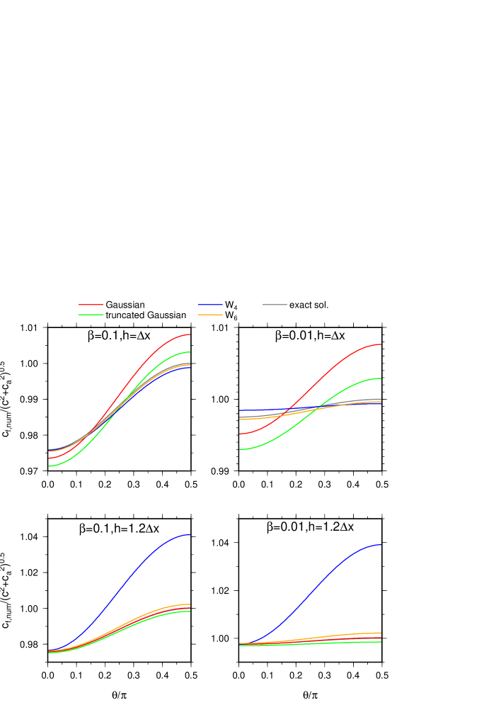
Figure 1: Phase velocity of the fast mode versus the angle between ${\bf k}$ and ${\bf B}_{0}$ for $(\beta,h)=(0.1,\Delta x)$, $(0.01,\Delta x)$, $(0.1,1.2\Delta x)$, and $(0.01,1.2\Delta x)$. The results with $\xi=1$ and $\xi=1/2$ are almost identical, and so only those with $\xi=1$ are presented. The red, green, blue, and orange lines correspond to the results using the Gaussian, truncated Gaussian, cubic spline, and quintic spline kernels. In each panel, the exact solutions are shown by the gray line.

4.1.2 Slow Mode

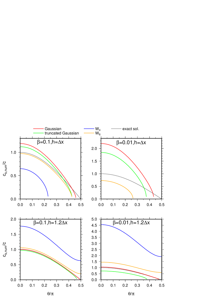
Figure 2: Phase velocity of the slow mode versus the angle between ${\bf k}$ and ${\bf B}_{0}$ for $(\beta,h)=(0.1,\Delta x)$, $(0.01,\Delta x)$, $(0.1,1.2\Delta x)$, and $(0.01,1.2\Delta x)$. The red, green, blue, and orange lines correspond to the results using the Gaussian, truncated Gaussian, cubic spline, and quintic spline kernels. In each panel, the exact solutions are shown by the gray line. All results are taken at $\xi=1$.

The slow mode exhibits completely different dispersion properties than the fast mode. Fig. 2 shows the numerical phase velocities of the slow mode as a function of the angle $\theta$ for various values of $\beta$ and $h$, and various kernel functions, with $\xi=1$. At $\theta=0$, the slow mode corresponds to the sound wave propagating in the direction parallel to ${\bf B}_{0}$. The phase velocity decreases with $\theta$ and gradually becomes the incompressible mode. At $\theta=\pi/2$, the phase velocity becomes zero. First, we focus on the cases with $h=\Delta x$ shown in the upper panels of Fig. 2. The results with $W_{4}$ are significantly underestimated for $\beta=0.1$ and leads to a numerical instability at $\beta=0.01$. Even for the smoother kernels ($W_{\mathrm{G}}$, $W_{\mathrm{tG}}$, $W_{6}$), the dispersion errors are significantly large and becomes worse for smaller $\beta$. Although only $W_{6}$ provides a better result for $\beta=0.1$, the stronger magnetic field ($\beta=0.01$) makes the results worse. From the lower left panel in Fig. 2, for $\beta=0.1$, larger $h$ ($h=1.2\Delta x$) improves the results with the smoother kernels while the result with $W_{4}$ does not improve. Also, in the case with larger $h$, for the stronger magnetic field ($\beta=0.01$), the dispersion errors become worse except for $W_{\mathrm{G}}$. In summary, the dispersion errors of the slow mode are large and becomes significant as $\beta$ decreases. A larger smoothing length makes the errors lower with every kernel except for the cubic spline, although large errors still remain for sufficiently low $\beta$. Thus, larger smoothing length cannot be an ultimate solution.

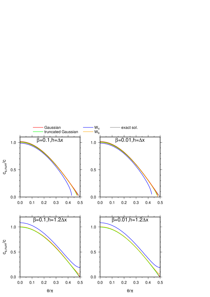
Figure 3: Phase velocity of the slow mode versus the angle between ${\bf k}$ and ${\bf B}_{0}$ for $(\beta,h)=(0.1,\Delta x)$, $(0.01,\Delta x)$, $(0.1,1.2\Delta x)$, and $(0.01,1.2\Delta x)$. The red, green, blue, and orange lines correspond to the results using the Gaussian, truncated Gaussian, cubic spline, and quintic spline kernels. In each panel, the exact solutions are shown by the gray line. All results are taken at $\xi=1/2$.

Fig. 3 is the same as Fig. 2 but setting $\xi=1/2$. All kernels can provide the correct phase velocities for all cases although the results with $W_{4}$ have relatively large errors. BOT04 have already investigated the dispersion properties for $\xi=1/2$, and their results are consistent with ours.

Figs. 2 and 3 reveal that SPM with $\xi=1$ exhibits significantly large dispersive errors that disappear if $\xi=1/2$ is used. This behavior can be qualitatively understood from the simple one-dimensional dispersion relation for $k_{y}=0$ ($\theta=0$) given by

$$\omega^{2}=\left\{2c^{2}+c_{\mathrm{a}}^{2}(2\xi-1)\right\}\left(\Psi^{xx}-\phi^{x}\psi^{x}\right)+c^{2}\phi^{x}\psi^{x}.$$ (33)

To obtain the correct phase velocity, $c$, the first term on the right-hand side of equation (33) should be negligible when compared with the second term. However, in contrast to the fast mode case, the coefficient of $(\Psi^{xx}-\phi^{x}\psi^{x})$ in equation (33) is much larger than that of $\phi^{x}\psi^{x}$ for low $\beta$ ($c_{\mathrm{a}}\gg c$). Thus, the first term can be important even if $|(\Psi^{xx}-\phi^{x}\psi^{x})/(\phi^{x}\psi^{x})|$ is sufficiently small. Note that the contribution of the magnetic field disappears only at $\xi=1/2$ in the first term of equation (33), and the dispersion relation is reduced to that without a magnetic field. That is why the errors are mostly eliminated for $\xi=1/2$, as shown in Fig. 3.

These findings in the long-wavelength limit suggest that the best choice for $\xi$ is 1/2, as SPM with $\xi=1$ suffers from significant errors.

4.2 Dispersion Relation

In this section, the overall dispersive properties of SPM are investigated.

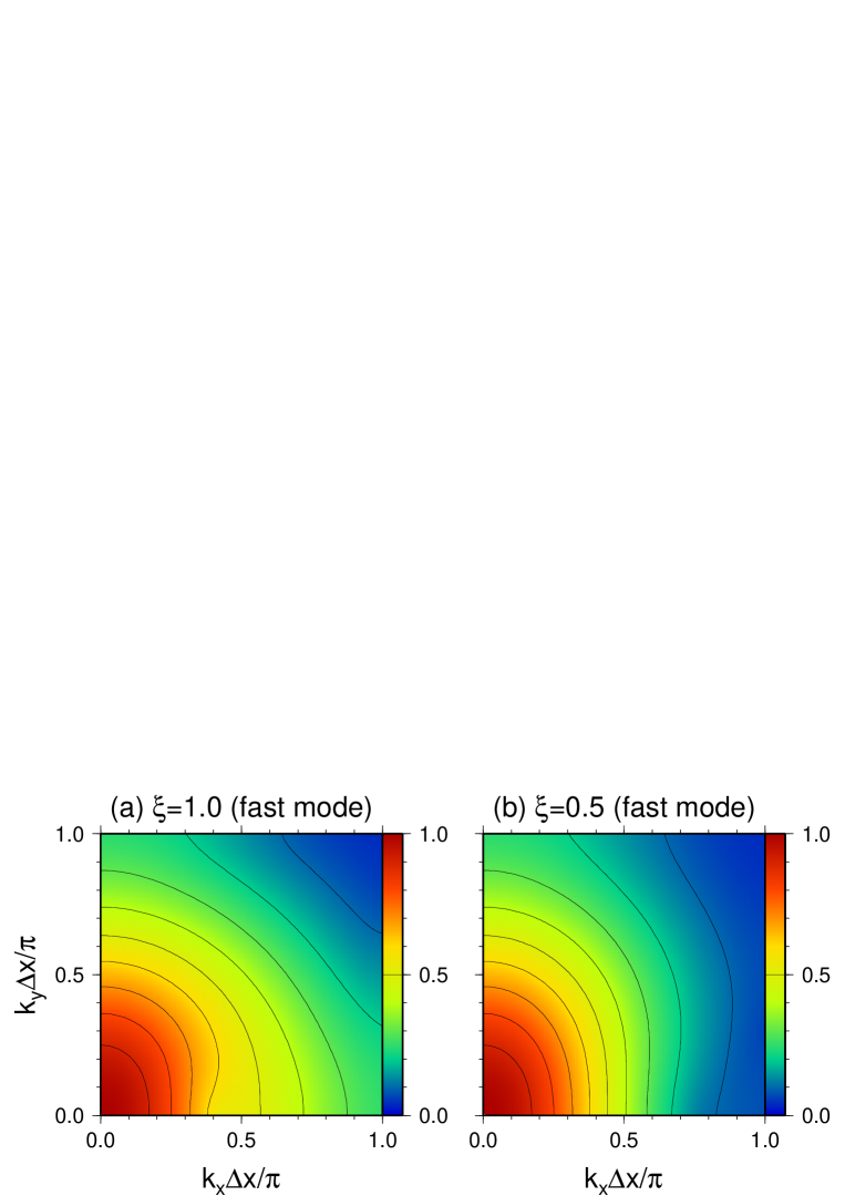
Figure 4: Color maps of the phase velocities of the fast mode in the $(k_{x}\Delta x/\pi,k_{y}\Delta x/\pi)$ plane for (a)$\xi=1$ and (b)$\xi=1/2$. The Gaussian kernel is considered. The parameters $\beta=0.1$ and $h=1.2\Delta x$ are used. In each panel, the color shows the numerical phase velocity normalized by the exact phase velocity depending on $\theta$. The gray region corresponds to the unstable region.

Figs. 4a and 4b show color maps of the numerical phase velocities of the fast mode in the $(k_{x}\Delta x/\pi,k_{y}\Delta x/\pi)$ plane for $\xi=1$ and $1/2$, respectively. The smoothing length is assumed to be $h=1.2\Delta x$, and the plasma $\beta$ value is fixed to be $\beta=0.1$. Here, we focus on the results with the Gaussian kernel. It is confirmed that the qualitative properties do not depend on the kernel functions. In Fig. 4, the numerical phase velocities are divided by the corresponding exact solutions depending on $\theta$. In both panels in Fig. 4, $c_{\mathrm{f,num}}/c_{\mathrm{f}}(\theta)$ has peaks at the origin and monotonically decreases with $|{\bf k}|$ at all $\theta$, where $c_{\mathrm{f}}$ is the exact phase velocity of the fast mode. The difference between the results with $\xi=1$ and $1/2$ is found only in the region where $|{\bf k}|\Delta x/\pi>0.5$ and $\theta\sim 0$. For $\xi=1/2$, $c_{\mathrm{f,num}}/c_{\mathrm{f}}$ declines more rapidly than it does for $\xi=1$. This behavior will be explained later. Thus, the dispersion relation of the fast mode does not depend much on the value of $\xi$. This is consistent with the findings in Section 4.1.1.

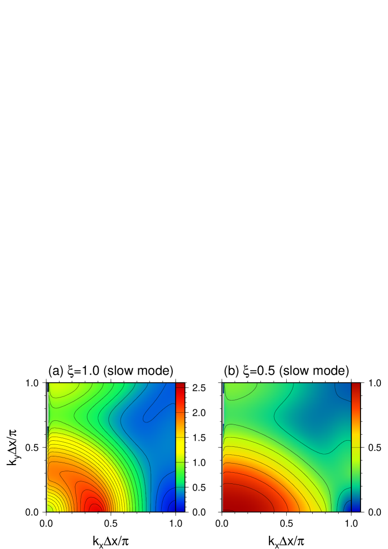
Figure 5: Color maps of the phase velocities of the slow mode in the $(k_{x}\Delta x/\pi,k_{y}\Delta x/\pi)$ plane for (a)$\xi=1$ and (b)$\xi=1/2$. The Gaussian kernel is considered. The parameters $\beta=0.1$ and $h=1.2\Delta x$ are used. In each panel, the color shows the numerical phase velocity normalized by the exact phase velocity depending on $\theta$. The gray region corresponds to the unstable region.

Next, the dispersion relations of the slow mode are investigated. Fig. 5 is the same as Fig. 4 but for the slow mode. First, the result with $\xi=1$, as shown in Fig. 5a, is investigated. Fig. 5a shows that $c_{\mathrm{s,num}}/c$ exhibits anomalous features, although $c_{\mathrm{s,num}}$ can reproduce the correct phase velocities in the long-wavelength limits for the Gaussian kernel (see the lower left panel in Fig. 2). $c_{\mathrm{s,num}}/c_{\mathrm{s}}$ increases from the origin with $|{\bf k}|$ especially in the direction parallel to ${\bf B}_{0}$ ($\theta\sim 0$). Around $|{\bf k}|\Delta x/\pi\sim 0.4$, $c_{\mathrm{s,num}}/c_{\mathrm{s}}$ reaches a maximum whose value is $\sim 2.5$ times larger than the exact solution. For larger $|{\bf k}|$ $(|{\bf k}|\Delta x/\pi>0.4$), $c_{\mathrm{s,num}}$ decreases with $|{\bf k}|$.

These anomalous features of the dispersion relation for $\xi=1$ completely disappear at $\xi=1/2$, as shown in Fig. 5b where $c_{\mathrm{s,num}}/c_{\mathrm{s}}$ monotonically decreases with $|{\bf k}|$ from the center.

Fig. 5 reveals that the phase velocities around $\theta=0$ strongly depend on $\xi$. To see this more clearly, the phase velocities at $\theta=0$ and $\theta=0.05$ are plotted in Fig. 6 as a function of $|{\bf k}|$. Fig. 6a shows the results with $\xi=1$. First, we focus on the case where $\theta=0$, shown by the solid lines. As mentioned above, the numerical phase velocities agree with the exact values for both the fast and slow modes. From $k=0$, $c_{\mathrm{f,num}}$ decreases with $k$ while $c_{\mathrm{s,num}}$ increases. At $k\Delta x/\pi\sim 0.4$, the two branches have the same phase velocity. Beyond this point, it can be clearly seen that the fast mode branch smoothly connects with the slow mode branch. This happens simply because larger (smaller) $\omega^{2}$ is referred to as the fast (slow) mode in this study, regardless of its eigenfunction. The “real” fast (slow) mode should be an incompressible (compressible) mode at $\theta=0$. By investigating the corresponding eigenfunctions, it is confirmed that the “real” fast and slow modes intersect at $k\Delta x/\pi\sim 0.4$. This means that the slow mode changes into an incompressible mode and the fast mode changes into a compressible mode beyond the intersection point. The dashed line in Fig. 6 indicates the results with $\theta=0.05$. We can see the mode exchange between the fast and slow branches around $k\Delta x/\pi\sim 0.4$. From the eigenfunctions, it is confirmed that the fast (slow) branch is changed into a compressible (incompressible) mode by the mode exchange. Fig. 6a indicates that the phase velocity of the compressible mode (the “real” slow mode) is supersonic $(>c_{\mathrm{s}})$ for all wavenumbers.

Fig. 7 shows the $\beta$-dependence of the maximum phase velocity of the compressible mode for $\xi=1$ and $\theta=0$. As shown in Fig. 6a, the “real” slow mode has an off-center peak. From Fig. 7, we can see that the maximum phase velocity increases with decreasing $\beta$. The maximum phase velocity for low $\beta$ is well fitted by $c_{\mathrm{a}}/2$ shown by the dashed line Fig. 7. This dependence clearly indicates that the enhancement of the phase speed of the compressible wave comes from the magnetic fields.

Fig. 6b shows the results for $\xi=1/2$. The phase velocity of the slow mode monotonically decreases with $k$. Also for $\xi=1/2$, the mode exchange occurs at larger $k$. From Figs.6a and 6b, the extended feature around $\theta\sim 0$ in $c_{\mathrm{f,num}}$ in Fig. 4a corresponds to a compressible mode with a large phase velocity ($>c_{\mathrm{s}}$) created by mode exchange.

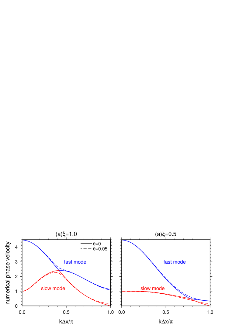
Figure 6: Dispersion relations for (a)$\xi=1$ and (b)$\xi=1/2$. The Gaussian kernel is used. In each panel, the blue and red lines corresponds to the fast and slow modes, respectively. The solid and dashed lines indicate the results with $\theta=0$ and $\theta=0.05$, respectively.

Figure 7: The $\beta$-dependence of the maximum phase velocity of the compressible mode for the $\xi=1$ and $\theta=0$ case. The Gaussian kernel is used. The dashed line indicates $c_{\mathrm{a}}/2$.

5 Numerical Experiments

Fig. 6 reveals that the dispersion relation is abnormal if $\xi=1$ is used. In Section 4.2, it is found that the compressible waves at short-wavelength propagate with supersonic velocities. In this section, to test this dispersive property, three simple test calculations are demonstrated.

5.1 Propagation of an Isolated Wave

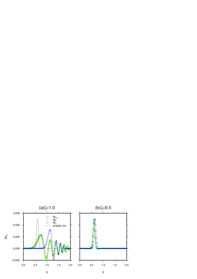
Figure 8: Dispersion relations for (a)$\xi=1$ and (b)$\xi=1/2$. In each panel, the blue and red lines correspond to the fast and slow modes, respectively. The solid and dashed lines indicate the results with $\theta=0$ and $\theta=0.05$, respectively.

Fist, test of the propagation of an isolated wave is performed. This is a severe test for the propagation of linear waves because an isolated wave is composed of many linear waves with different wavelengths. Thus, if the sound speed numerically has a $k$-dependence, the shape of an isolated wave is expected to change during its propagation. In other words, the deformation of an isolated wave clearly shows the dispersion errors.

In the unperturbed state, the particles are distributed in a rectangular lattice in the domain of $[-2,2]\times[-1,1]$. The density and pressure are assumed to be 1. A uniform magnetic field is introduced in the $x$-direction, and its strength is set such that $\beta$ is 0.1. A velocity perturbation given by $\delta v=0.01\exp(-(x/3h)^{2})$ is added. The two isolated waves propagate outward from the origin. As the sound wave does not have dispersion, the two isolated waves should keep their shape with the sound speed ($c=1$) as they propagate. Cha and Whitworth [21] did the same test calculation without magnetic fields.

Fig. 8a shows a snapshot of the velocity perturbation at $t=0.6$ for $\xi=1$. Only the isolated wave propagating rightward is plotted. The gray lines indicate the exact solution. The colors indicate the difference of the kernel functions. For $\xi=1$, with all kernel functions, the isolated waves break into smaller waves that propagates at supersonic velocities. This dispersive property is consistent with the results of linear analysis. The results with $W_{6}$ are almost identical to that with $W_{\mathrm{tG}}$. The isolated wave with $W_{4}$ shows a larger speed, as expected in Fig. 5. On the other hand, for $\xi=1/2$, there is no destruction of the isolated wave, and the results agree with the exact solution quite well, although the result with $W_{4}$ shows a slightly larger phase velocity. This is explained by the linear analysis (see the lower left panel of Fig. 3). These findings suggest that the optimal choice for $\xi$ is $1/2$. Otherwise SPM provides completely incorrect results for the wave propagation.

5.2 Colliding Flow Test

The linear analysis is valid only for the linear waves. In this test, we consider a colliding flow test that involves shock waves. We investigate whether the dispersive errors affect the shock structures or not. The computational domain is $-1<x<1$, $-0.0625<y<0.0625$, and the periodic boundary condition is imposed in the $y$-direction. Initially, the density is uniform, and the gas moves toward $x=0$ from both directions with a velocity $\pm 3.75$. The corresponding Mach number is $4$. The initial magnetic field is ${\bf B}=\left(\sqrt{8\pi/\beta},0\right)$. As the magnetic field is parallel to the $x$-direction, it should not affect the gas dynamics. The truncated Gaussian kernel is used. We consider two cases: $\beta=0.1$ and $0.01$. In the exact solution, two shock waves propagates outward from $x=0$. In this test, we investigate how the strong parallel magnetic field numerically affects the gas motion. The initial particle distribution is set to be a random distribution that is relaxed until the density dispersion is sufficiently small. In this test, a Riemann solver is used to capture shock waves. The hyperbolic divergence cleaning method [22, 6] is also used.

Fig. 9a shows the results with $\xi=1$ and $\xi=1/2$ for $\beta=0.1$. The black line indicates the exact solution. Both cases agree with the exact solution quite well. This is because the shock jump condition is determined only by mass and momentum conservation laws, regardless of their dispersive properties. For the stronger magnetic field case $(\beta=0.01)$, the effect of the dispersive errors is shown in Fig. 9b. For $\xi=1/2$, the density of the shocked gas can reproduce the exact solution reasonably well within an error of $2\%$. This small error occurs due to the perpendicular magnetic field $B_{y}$ numerically generated at the shock front. It works as an additional pressure, leading to the smaller density jump. For $\xi=1$, the density profile is quite different from the exact solution. The shock fronts broaden and small waves propagate toward the upstream with a supersonic velocity larger than the converging velocity $3.75$. This can be understand by Fig. 7. For $\beta=0.01$, the maximum phase velocity of the compressible wave is $\sim c_{\mathrm{a}}/2\sim 7$, which is larger than the converging velocity. Thus, waves can propagate toward upstream against the converging flow.

From this converging flow test, it is found that given $\beta$, there is a minimum shock speed below which waves with short wavelengths propagate upstream and disturb the preshock gas. The minimum shock speed corresponds to the maximum phase velocity of the compressible wave, or $c_{\mathrm{a}}/2$ derived from the linear analysis (see Fig. 7). In other words, if the Alfvén Mach number is smaller than 0.5, the dispersive errors are serious.

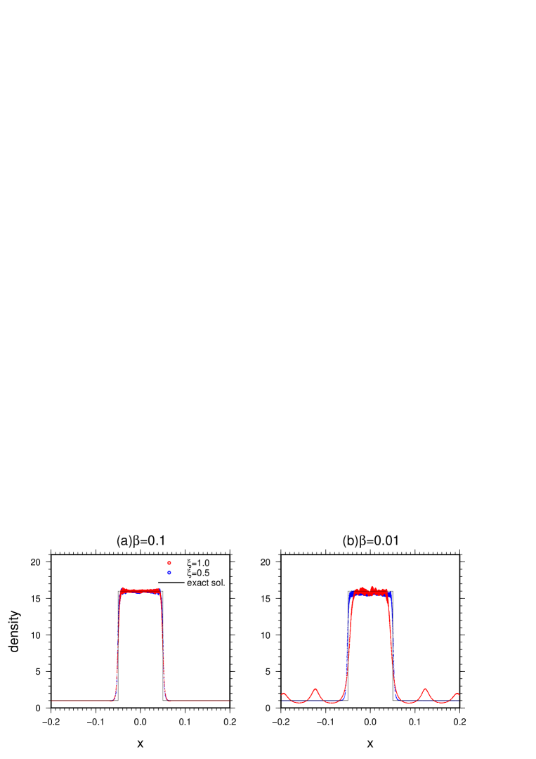
Figure 9: Density profiles at $t=0.2$ for (a)$\beta=0.1$ and (b)$\beta=0.01$. Each point corresponds to an SPH particle. In each panel, the red and blue lines corresponds to the results with $\xi=1$ and $\xi=1/2$, respectively. The green lines indicate the exact solution.

5.3 Hydrostatic Equilibrium Under An External Gravity

The dispersion errors originate from the fact that a parallel magnetic field numerically works as an additional repulsive force. This indicates that the errors can be important not only for waves but also for hydrostatic structures. Thus, in this test, we investigate whether SPM reproduces a hydrostatic structure under an external gravity, $g_{x}=-2\tanh(x)$. As the initial condition, we consider a uniform static gas with a uniform magnetic field in the $x$-direction. The amplitude of the magnetic field is $\sqrt{8\pi/\beta}$. The calculation domain is $-2<x<2$ and $-1/4<y<1/4$. The truncated Gaussian kernel is used. A periodic boundary condition is imposed in the $y$-direction, and the wall boundary condition is imposed in the $x$-direction. The initial particle configuration is set to be a settled random distribution. Because of the external gravity, the plasma accumulates toward the midplane ($x=0$). Finally, the density profile is expected to relax to the hydrostatic equilibrium profile, $\rho_{\mathrm{eq}}(x,y)=1/\cosh(x)^{2}$. To avoid an undesirable oscillation in the relaxation phase, we add a small drag force, $-0.005{\bf v}/\Delta t$, to the equation of motion. If the maximum velocity becomes smaller than $0.001$, the calculations are terminated.

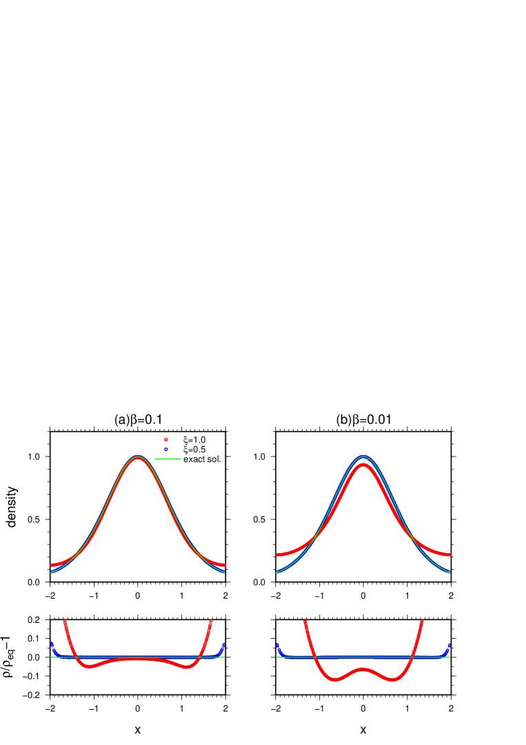
Figure 10: (Upper panels) Density profiles for (a)$\beta=0.1$ and (b)$\beta=0.01$. (Lower panels) Fractional residual, $\rho(x)/\rho_{\mathrm{eq}}-1$. Each point corresponds to an SPH particle. In each panel, the red and blue lines corresponds to the results with $\xi=1$ and $\xi=1/2$, respectively. The green lines indicate the hydrostatic profile.

The upper panel of Fig. 10a shows the obtained density profiles for $\beta=0.1$. The lower panel of Fig. 10a indicates the fractional residual, $\rho(x)/\rho_{\mathrm{eq}}(x)-1$. The result with $\xi=1/2$ agrees with the hydrostatic profile within sufficiently small error. The small deviation around $x=\pm 2$ comes from the boundary condition. Also for $\xi=1$, SPM reproduces the hydrostatic profile reasonably well, although the density in the central region is underestimated and the low density tails are overestimated. However, this tendency becomes prominent for $\beta=0.01$, as shown in Fig. 10b. The density profile with $\xi=1$ exhibits a more extended profile than $\rho_{\mathrm{eq}}(y)$. On the other hand, even for $\beta=0.01$, SPM with $\xi=1/2$ can produce the correct profile. From the test, it is found that the hydrostatic profiles along the magnetic fields are broadened by the artificial repulsive force if $\xi=1$ is used.

6 Discussion

6.1 Stability Against Particle Disorder

The test calculations demonstrated in Section 5 show that SPM with $\xi=1/2$ removes dispersion errors. However, in a realistic situation where a blast wave propagates in a strongly magnetized medium, Tricco and Price [10] (hereafter TP12) found that SPM with $\xi<1$ produces numerical fluctuations behind the slow shocks and at the contact discontinuity. They found that a value of $\xi=1$ leads to stable results. This is because the repulsive force is weaker for SPM with smaller $\xi$ , leading to the particle disorder.

To investigate the stability against the particle disorder in SPM with $\xi=1/2$, we perform the same blast wave test as in TP12. The total particle number is $512\times 512$. Fig. 11a and 11b show the density maps at $t=0.03$ for $\xi=1$ and $\xi=1/2$, respectively. The truncated Gaussian kernel is used. One can see that the result with $\xi=1/2$ is quite similar to that with $\xi=1$. As shown in Section 5.2, SPM can treat shock waves even for $\xi=1$ as long as the Alfvén Mach number is larger than 0.5. Thus, it is difficult to identify the dispersion errors in this test.

Note that the significant particle disorder found by TP12 does not appear in Fig. 11b. Although this discrepancy may come from the difference of treatment of the numerical dissipations between GSPM and their scheme, the exact reason is still uncertain. However, also in the GSPM, the result with $\xi=1$ is smoother than that with $\xi=1/2$. Thus, it is possible that GSPM with $\xi=1/2$ suffers from the serious particle disorder in more extreme situations. The best choice of $\xi$ depends on situations from the point of view of accuracy and stability. As shown in the linear analysis, the dispersive errors are serious in slow waves propagating along magnetic fields. Thus, for example, to simulate a sub-Alfvénic turbulence in low $\beta$ plasma, a value of $\xi=1/2$ should be adopted. On the other hand, in dynamical situations where strong shock waves are important such as the blast wave test, the dispersive errors are not serious if the Alfvén Mach number is larger than 0.5 (see Section 5.2). In these cases, a value of $\xi=1$ is acceptable.

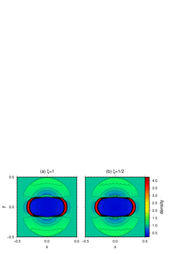
Figure 11: Density maps of the blast wave test at $t=0.03$ for (a)$\xi=1$ and (b)$\xi=1/2$. The truncated Gaussian kernel is used. A value of $\xi=1/2$ is used.

6.2 Comparison with Other SPM Formulation

Besides the approach by Børve, Omang, and Trulsen [9], Morris [16] proposed the following formulation;

$$\frac{dv_{a}^{\mu}}{dt} = -\sum_{b}m_{b}\left(\frac{P_{a}+\frac{1}{8\pi}B_{a}^{2}}{\Omega_{a}\rho_{a}^{2}}\nabla_{a}^{\nu}W_{ab}(h_{a})+\frac{P_{b}+\frac{1}{8\pi}B_{b}^{2}}{\Omega_{b}\rho_{b}^{2}}\nabla_{a}^{\nu}W_{ab}(h_{b})\right)$$ (34)

$$+ \frac{1}{4\pi}\sum_{b}m_{b}\left(\frac{B_{b}^{\mu}B_{b}^{\nu}-B_{a}^{\mu}B_{a}^{\nu}}{\rho_{a}\rho_{b}}\right)\frac{\nabla_{a}^{\nu}W_{ab}(h_{a})+\nabla_{a}^{\nu}W_{ab}(h_{b})}{2}.$$

In his formulation, the conservative form is used in the isotropic part of the stress tensor while the non-conservative form is used in the remaining part. Thanks to the non-conservative term, his formulation is free from the numerical instability. In this section, we compare the dispersion relations between the Morris formulation (SPM_Morris) and the conservative form with the correction term (SPM_corr). Linearizing equation (34), one obtains the following dispersion relation;

$$\mathrm{det}\left(\omega^{2}\delta^{\mu\nu}+A^{\mu\nu}\right)=0,$$ (35)

where

$$A^{\mu\nu} = \frac{2}{\rho_{0}}\left(P_{0}+\frac{B_{0}^{2}}{8\pi}\right)\left(\phi^{\mu}\psi^{\nu}-\Psi^{\mu\nu}\right)-\frac{\phi^{\mu}}{\rho_{0}}\left[P_{0}\psi^{\nu}+\frac{1}{4\pi}\left(B_{0}^{2}\psi^{\nu}-B_{0}^{\eta}\psi^{\eta}B_{0}^{\nu}\right)\right]$$ (36)

$$+ \frac{B_{0}^{\eta}{\psi}^{\eta}}{4\pi}\left(B_{0}^{\zeta}\psi^{\zeta}\delta^{\mu\nu}-B_{0}^{\mu}\psi^{\nu}\right).$$

Fig. 12 shows the color map of the numerical phase velocities of the slow mode using SPM_Morris in the $(k_{x}\Delta x/\pi,k_{y}\Delta x/\pi)$ plane. The smoothing length is assumed to be $h=1.2\Delta x$, and the plasma $\beta$ value is fixed to be $\beta=0.1$. The Gaussian kernel is considered. One can see that the behavior of $c_{\mathrm{s,num}}$ is quite similar to that in SPM_corr with $\xi=1$ (see Fig. 5a). The dispersion relations have an off-center peak of $c_{\mathrm{s,num}}$ around $\theta\sim 0$. Thus, the SPM formulation by Morris [16] also suffers from the dispersive errors. This behavior can be qualitatively understood from equation (36). The first term on the right-hand side of equation (36) that leads to most of the dispersive errors becomes large compared with other terms for low $\beta$ plasma. Note that in SPM_corr the corresponding term proportional to $\left(\phi^{\mu}\psi^{\nu}-\Psi^{\mu\nu}\right)$ is negligible if $\xi=1/2$ is used.

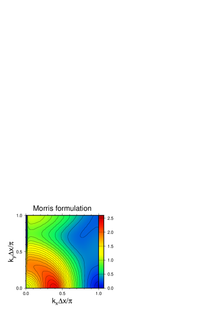
Figure 12: Color maps of the phase velocities of the slow mode using SPM_Morris in the $(k_{x}\Delta x/\pi,k_{y}\Delta x/\pi)$ plane. The Gaussian kernel is considered. The parameters $\beta=0.1$ and $h=1.2\Delta x$ are used. The color shows the numerical phase velocity normalized by the exact phase velocity depending on $\theta$.

7 Summary

In this study, we have investigated the dispersive properties of SPM with a correction term introduced to remove numerical instability in a strongly magnetized medium [9]. The size of the correction term is parametrized by $\xi$ (see equation (2)). The findings in this study are summarized as follows:

• As numerically found by Børve, Omang, and Trulsen [12], the minimum value of $\xi$ for removing the numerical instability is analytically derived as a function of the plasma $\beta$ value in Section 3.1.1.

• For the fast modes, it is found that SPM can reproduce correct phase velocities regardless of $\xi$. The dispersion properties are similar to those without magnetic fields.

• The phase velocities of the slow modes is shown to significantly depend on $\xi$. For $\xi=1$, which is used in most schemes, it is found that SPM suffers from significant dispersion errors with all kernel functions. The dispersion errors become worse for a lower value of $\beta$. In the long-wavelength limit $(\lambda/2\pi=10^{3}\Delta x/\pi)$, the numerical phase velocities are largely different from the exact values especially for the cubic spline kernel. A larger smoothing length and a smoother kernel functions are not ultimate solution if $\beta$ is sufficiently small (see Fig. 2). The dispersion relations have an off-center peak of the phase velocities around $|k|\Delta x/\pi\sim 0.4$ and $\theta\sim 0$, where $\theta$ is the angle between ${\bf k}$ and ${\bf B}_{0}$. Furthermore, the phase velocities are supersonic for all wavenumbers above the Nyquist wavenumber $\pi/\Delta x$ (see Fig. 5). The reason for this anomalous behavior is that a parallel magnetic field numerically works as an additional repulsive force and the phase velocities of the slow wave become supersonic. This fact can be understood by examining the dispersion relation with respect to the slow wave propagating along a magnetic field.

  On the other hand, for $\xi=1/2$, the dispersion errors found for $\xi=1$ completely disappear. This can be understood analytically from the dispersion relation.

• To confirm the findings of the linear analysis, several simple numerical experiments are demonstrated. For the tests of linear isolated waves and hydrostatic equilibrium, SPM with $\xi=1$ leads to unphysical results while the exact solutions can be reproduced for $\xi=1/2$. On the other hand, SPM with $\xi=1$ can treat the parallel shock waves if Alfvén Mach number is larger than 0.5. This is because the shock condition is determined only by the conservation properties and slow waves cannot propagate toward upstream. If the shock speeds are smaller, waves propagate upstream against the flow and cause disturbances. These results are consistent with the linear analysis.

This study clearly shows that corrected SPM with $\xi=1$ over-stabilizes the numerical instability and significantly modifies the dispersion properties of the slow modes. To eliminate such dispersion errors, we suggests that $\xi=1/2$ is the best choice. These abnormal dispersion properties have not been found in the previous works, (e.g., the blast wave tests used to test the capability of schemes for low $\beta$) because, as shown in Section 5.2, SPM can treat shock waves even for $\xi=1$ as long as the shock speed is large. Thus, it is difficult to identify the dispersion errors found in this study from the blast wave test. The errors can be serious; for instance, in sub-Alfvénic turbulence for low $\beta$ plasma, the phase velocity of the waves propagating along magnetic fields may be significantly overestimated.

The linear analysis and the numerical experiments suggest that the best choice of $\xi$ is 1/2 from the point of view of accuracy. However, as discussed in Section 6.1, SPM with $\xi=1/2$ tends to less stable against particle disorder because of the small repulsive force. In dynamical environments where strong shock waves are important, a value of $\xi=1$ is acceptable if the Alfvén Mach number is larger than 0.5.

References

- Lucy [1977] L. B. Lucy, A numerical approach to the testing of the fission hypothesis, AJ 82 (1977) 1013.
- Gingold and Monaghna [1977] R. A. Gingold, J. J. Monaghan, Smoothed particle hydrodynamics: theory and application to non-spherical stars, MNRAS 171 (1977) 375–389.
- Price and Monaghan [2005] D. J. Price, J. J. Monaghan, Smoothed Particle Magnetohydrodynamics - III. Multidimensional tests and the .B= 0 constraint, MNRAS 364 (2005) 384–406.
- Dolag and Stasyszyn [2009] K. Dolag, F. Stasyszyn, An MHD GADGET for cosmological simulations, MNRAS 398 (2009) 1678–1697.
- Iwasaki and Inutsuka [2011] K. Iwasaki, S. Inutsuka, Smoothed particle magnetohydrodynamics with a Riemann solver and the method of characteristics, MNRAS 418 (2011) 1668–1688.
- Iwasaki and Inutsuka [2015] K. Iwasaki, S. Inutsuka, in preparation.
- Phillips and Monaghan [1985] G. J. Phillips, J. J. Monaghan, A numerical method for three-dimensional simulations of collapsing, isothermal, magnetic gas clouds, MNRAS 216 (1985) 883–895.
- Morris [1996] J. P. Morris, A study of the stability properties of smooth particle hydrodynamics, PASA 13 (1996) 97–102.
- Børve, Omang, and Trulsen [2001] S. Børve, M. Omang, J. Trulsen, Regularized Smoothed Particle Hydrodynamics: A New Approach to Simulating Magnetohydrodynamic Shocks, ApJ 561 (2001) 82–93.
- Tricco and Price [2012] T. S. Tricco, D. J. Price, Constrained hyperbolic divergence cleaning for smoothed particle magnetohydrodynamics, J. Comput. Phys 231 (2012) 7214–7236.
- Price [2012] D. J. Price, Smoothed particle hydrodynamics and magnetohydrodynamics, J. Comput. Phys 231 (2012) 759–794.
- Børve, Omang, and Trulsen [2004] S. Børve, M. Omang, J. Trulsen, Two-dimensional MHD Smoothed Particle Hydrodynamics Stability Analysis 153 (2004) 447–462.
- Barnes, Kawata, and Wu [2012] D. J. Barnes, D. Kawata, K. Wu, Cosmological simulations using GCMHD+, MNRAS 420 (2012) 3195–3212.
- Børve, Omang, and Trulsen [2006] S. Børve, M. Omang, J. Trulsen, Multidimensional MHD Shock Tests of Regularized Smoothed Particle Hydrodynamics, ApJ 652 (2006) 1306–1317.
- Balsara [1995] D. S. Balsara, von Neumann stability analysis of smooth particle hydrodynamics–suggestions for optimal algorithms, J. Comput. Phys 121 (1995) 357–372.
- Morris [1996] J. P. Morris, PhD thesis, Monash University.
- Stone and Norman [1992] J. M. Stone, M. L. Norman, ZEUS-2D: A Radiation Magnetohydrodynamics Code for Astrophysical Flows in Two Space Dimensions. II. The Magnetohydrodynamic Algorithms and Tests 80 (1992) 791.
- Schoenberg [1946] I. J. Schoenberg, Contributions to the problem of approximation of equidistant data by analytic functions. A: on the problem of smoothing or graduation - a 1st class of analytic approximation formulae , Q. Appl. Math. 4 (1946) 45.
- Monaghan and Lattanzio [1985] J. J. Monaghan, J. C. Lattanzio, A refined particle method for astrophysical problems, A&A 149 (1985) 135–143.
- Monaghan [1989] J. J. Monaghan, On the problem of penetration in particle methods, J. Comput. Phys 82 (1989) 1–15.
- Cha and Whitworth [2003] S.-H. Cha, A. P. Whitworth, Implimentations and tests of Godunov-type particle hydrodynamics , MNRAS 340 (2003) 73.
- Iwasaki and Inutsuka [2013] K. Iwasaki, S. Inutsuka, Vol. 474 of Astronomical Society of the Pacific Conference Series, 2013, p. 239.