Fragmentation properties of two-dimensional Proximity Graphs considering random failures and targeted attacks

Abstract

The pivotal quality of proximity graphs is connectivity, i.e. all nodes in the graph are connected to one another either directly or via intermediate nodes. These types of graphs are robust, i.e., they are able to function well even if they are subject to limited removal of elementary building blocks, as it may occur for random failures or targeted attacks. Here, we study how the structure of these graphs is affected when nodes get removed successively until an extensive fraction is removed such that the graphs fragment. We study different types of proximity graphs for various node removal strategies. We use different types of observables to monitor the fragmentation process, simple ones like number and sizes of connected components, and more complex ones like the hop diameter and the backup capacity, which is needed to make a network $N-1$ resilient. The actual fragmentation turns out to be described by a second order phase transition. Using finite-size scaling analyses we numerically assess the threshold fraction of removed nodes, which is characteristic for the particular graph type and node deletion scheme, that suffices to decompose the underlying graphs.

I Introduction

The pivotal issue of standard percolation Stauffer (1979); Stauffer and Aharony (1992) is connectivity. A basic example is $2D$ random site percolation, where one studies a lattice in which a random fraction of the sites is “occupied”. Clusters composed of adjacent occupied sites are then analyzed regarding their geometric properties. Depending on the fraction $p$ of occupied sites, the geometric properties of the clusters change, leading from a “fragmented” phase with rather small and disconnected clusters to a phase, where there is basically one large connected cluster covering the lattice. Therein, the appearance of an infinite, i.e. percolating, cluster is described by a second-order phase transition.

Similar to the issue of connectivity is the robustness, i.e. the ability of networks to function well even if they are subject to random failures or targeted attacks of their elementary building blocks, e.g., node removal. This is of particular importance for more applied real-world networks, which may fail even if they are still connected, e.g., when the dynamics of nodes is not synchronous due to an failure. Also, many real-world networks are not embedded in two-dimensions, they may even exhibit an infinite-dimensional, i.e., mean-field structure. E.g., electrical power grids must ensure power supply for entire resident population Albert et al. (2004), urban road networks Jiang and Claramunt (2004) and airline networks Choi et al. (2006) facilitate social and economical interaction, and the internet Barabási et al. (2000), which has become essential in almost all aspects of life. In general, networks are represented by a set of nodes, i.e. the elementary building blocks of a network, and pairs of nodes might be joined by edges. One possibility to characterize a network (or graph for that matter) is by means of its degree distribution, where the degree of a node refers to the number of its adjacent neighbors. Several real-world networks, such as the hyperlink-network of the internet, exhibit a scale-free degree distribution Barabási et al. (2000). During the last decade, various studies have been published that focus on this prototypical type of degree distribution. In particular, the fragmentation properties of scale-free Barabási-Albert (BA) networks Albert et al. (2000); Callaway et al. (2000); Crucitti et al. (2004a); Gallos et al. (2005); Holme et al. (2002); Cohen et al. (2001) (and also of several other ones Huang et al. (2011); Kurant et al. (2007); Paul et al. (2004); Shargel et al. (2003); Tanizawa et al. (2012)) have been put under scrutiny. In the aforementioned articles, different node-removal strategies have been considered to investigate the fragmentation properties of the considered networks. It turns out that scale-free networks are robust against random node removals, but very vulnerable to intentional attacks targeting particular “important” nodes. Note that there are many different local and global measures to quantify whether a node is important. Popular choices are, e.g., the degree of a node, its betweenness-centrality Brandes (2008) (subject to a particular metric used to measure the length of shortest paths between pairs of nodes), or, somewhat more specific to the hyperlink structure of the internet, the “PageRank” Page et al. (1999) relevance measure for web pages.

In the presented work we focus on types of networks, which are completely different from scale free graphs. The networks considered here are constructed from sets of points distributed in the two-dimensional Euclidean plane. More precisely, we consider three types of proximity graphs, namely relative neighborhood graphs (RNGs) Toussaint (1980), Gabriel graphs (GGs) Gabriel and Sokal (1969), and Delaunay triangulations (DTs) Sibson (1978). These are planar graphs Essam and Fisher (1970) where pairs of nodes are connected by undirected edges if they are considered to be close in some sense (see definitions in Sec. II). In addition, we consider also a certain type of (non planar) geometric random network, termed minimum-radius graph (MR), where pairs of nodes are connected if their distance does not exceed a particular threshold value. The above proximity graphs where already studied in different scientific fields such as the simulation of epidemics Toroczkai and Guclu (2007), percolation Bertin et al. (2002); Becker and Ziff (2009); Billiot et al. (2010); Melchert (2013), and message routing and information dissemination in ad-hoc networking Jennings and Okino (2002); Santi (2005); Li et al. (2005); Rajaraman (2002). To elaborate on the latter point, proximity graphs find application in the construction of planar “virtual backbones” for ad-hoc networks, i.e. collections of radio devices without fixed underlying infrastructure, along which information can be efficiently transmitted Karp and Kung (2000); Bose et al. (2001); Jennings and Okino (2002); Yi et al. (2010); Kuhn et al. (2003). Routing with guaranteed node-to-node connectivity (at least in a multi-hop manner) is especially important to ensure a complete broadcast of information in ad-hoc networks Jennings and Okino (2002). Here, we consider three types of node removal strategies with different levels of severity, see Sec. III, and we numerically assess the threshold fraction of removed nodes (characteristic for the particular graph type and node deletion scheme) that suffices to decompose the underlying graphs into “small” clusters.

The remaining article is organized as follows. In Sec. II we introduce the four different graph types that were considered in the presented study. In Sec. III we describe the three node-removal strategies that were used in order to characterize the fragmentation process for each of these graph types. In Sec. IV we introduce the observables that were recorded during the fragmentation procedure and we list the results of our numerical simulations. Finally, Sec. V concludes with a summary.

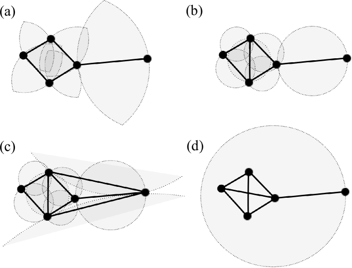
Figure 1: Examples of the four different graph types for a small set of $N=5$ nodes (see text for details). (a) instance of a RNG, where for all pairs of nodes that will be connected under the respective linking-rule, the respective lune is depicted in gray. (b) instance of a GG, where for all pairs of nodes that will be connected under the respective linking-rule, the circle that helps in the decision making process is depicted in gray. (c) instance of a DT, where the gray shaded circles are exemplary for those that might aid in the decision making process. (d) instance of a MR, where the linking range $r$ is depicted (gray circle) for a single node only (all other nodes exhibit the same linking range).

II Graph Types

Subsequently we introduce four different types of graphs for a planar set of, say, $N$ points and we characterize the fragmentation process on each of these graph types following three different node-removal strategies, detailed in Sec. III. Three of these graph types, introduced in Subsects. II.1 through II.3 belong to the class of proximity graphs Jaromczyk and Toussaint (1992). The fourth graph type, detailed in Subsect. II.4, is a particular type of a random geometric graph. Below, a graph is referred to as $G=(V,E)$, where $V$ comprises its node-set ($N=|V|$; where $N$ is also referred to as “system size”), and where $E$ ($M=|E|$) signifies the respective edge-set Essam and Fisher (1970). Each of the $N$ nodes $u\in V$ represents a point in the two-dimensional unit square for which the coordinates $u_{x}$ and $u_{y}$ are drawn uniformly and independently at random. So as to compute the distance ${\rm dist}(u,v)$ between two nodes $u,v\in V$ we consider the Euclidean metric under which ${\rm dist}(u,v)=[(u_{x}-v_{x})^{2}+(u_{y}-v_{y})^{2}]^{1/2}$. We further consider open boundary conditions. Thus an increase of the system size corresponds to increasing the density of nodes on the unit square. On the other hand, so as to maintain the density of nodes while increasing $N$, the networks can be pictured as having an effective side-length $L=\sqrt{N}$. A common feature of these four types of graphs is that their edge-set encodes proximity information regarding the close neighbors of the terminal nodes of a given edge. The different graph types can be distinguished by the precise linking-rule that is used to construct the edge-set for a given set of nodes. In this section the linking-rules that define the four types of proximity graphs will be detailed.

II.1 Relative Neighborhood Graphs (RNGs)

One particular proximity graph type that will be considered subsequently is the relative neighborhood graph (RNG) Toussaint (1980). In order to determine whether in the construction procedure for an instance of a RNG two nodes $u,v\in V$ need to be connected to each other, it is necessary to check if there is a third node $w\in V\setminus\{u,v\}$ with ${\rm dist}(u,w)\leq{\rm dist}(v,u)$ and ${\rm dist}(v,w)\leq{\rm dist}(v,u)$. If such a node $w$ does not exist, $u$ and $v$ will get linked. In geometrical terms, for each pair $u$ and $v$ of points, the respective distance $\rm{dist}(u,v)$ can be used to construct the lune ${\rm lune}(u,v)$. The lune is given by the intersection of two circles with equal radius $\rm{dist}(u,v)$, centered at $u$ and $v$, respectively. If no other point $w\in V\setminus\{u,v\}$ lies within ${\rm lune}(u,v)$, i.e. if the lune is empty, both nodes are connected by means of an edge. To facilitate intuition, an example of a RNG for a small set of $N=5$ nodes is sketched in Fig. 1(a). A larger example that illustrates the principal structure of a RNG is shown in Fig. 2(a).

II.2 Gabriel Graphs (GGs)

Another proximity graph that will be considered in this article is the Gabriel graph (GG) Gabriel and Sokal (1969); Bertin et al. (2002). To determine whether in the construction procedure for an instance of a GG two nodes $u,v\in V$ need to be connected, $\rm{circ}(u,v)$, i.e. the smallest of all possible circles which embeds both nodes is considered, which has a diameter $\rm{dist}(u,v)$. These two nodes will be connected unless there is another node $w$ which is located within the area enclosed by ${\rm circ}(u,v)$. To facilitate intuition, the linking rule for the GG is illustrated in Fig. 1(b). A larger example that illustrates the principal structure of a GG is shown in Fig. 2(b). Further, note that the GG is a super-graph of the RNG. This is due to the circumstance that $\rm{circ}(u,v)$, which is relevant in the construction procedure of a GG instance for a given set of nodes encloses a subarea of $\rm{lune}(u,v)$, being relevant in the construction procedure of the corresponding RNG instance (compare the grey shaded surfaces in Figs. 1(a,b)). Therefore, all edges contained in the RNG are also included in the GG. Note that this can also be seen in Figs. 2(a,b).

II.3 Delaunay Triangulations (DTs)

The construction of the Delaunay triangulation (DT; also a type of proximity graph) Sibson (1978) is quite similar. Two nodes $u,v\in V$ will be connected if any circle exists which embeds $u$ as well as $v$ but no further nodes. To facilitate intuition, the result of this linking-rule is shown in Fig. 1(c). A larger example that illustrates the principal structure of a DT is shown in Fig. 2(c). From the definition of these linking-rules, since the GG graph also involves the construction of a circle, it is evident that an instance of a DT for a given set of nodes must be a super-graph of the corresponding GG instance. As a consequence, being a sub-graph of the GG, the RNG is also a sub-graph of the DT. This can be observed in Figs. 1(a-c) (Figs. 2(a-c)), where the RNG, GG and DT are illustrated for the same set of $N=5$ ($100$) nodes.

Figure 2: Examples of the four different graph types for the same set of $N=100$ nodes, distributed uniformly at random in the 2D unit square. (a) RNG, (b) GG, (c) DT, and (d) MR.

II.4 Minimum Radius Graphs (MRs)

The fourth network topology that will be considered is the minimum radius graph (MR). In the construction procedure of an instance of a MR, two nodes $u,v\in V$ will be joined by an edge, if ${\rm dist}(u,v)\leq r$. Therein, the “connectivity radius” $r$ specifies the smallest possible value which ensures that all nodes are connected to one another, possibly in a multi-hop manner. It becomes evident from Figs. 1(d) and 2(d) that, in contrast to the previous graphs, the MR might feature crossing edges.

II.5 Graph construction

In order to construct the RNG and GG, we made use of the sub-graph hierarchy ${\rm RNG}\subset{\rm GG}\subset{\rm DT}$. I.e., for a given set of nodes we first obtained the DT by means of the Qhull computational geometry library Barber (1995) (the DT for a set of $N$ points can be computed in time $O(N\log(N))$ Preparata and Shamos (1985); Barber (1995)) and then pruned the resulting edge-set $E$ until the linking requirements of GG or RNG are met. Here, we amend the naive implementation of this two-step procedure Toussaint (1980), yielding an algorithm with running time $O(N^{2})$, by means of the “cell-list” method Melchert (2013), resulting in a sub-quadratic running time. In this regard, note that Ref. Jaromczyk and Toussaint (1992) provides an overview of several algorithmic approaches for the construction of RNGs and GGs. Finally, note that RNGs and GGs can be found as the limiting cases of a parameters family of proximity graphs, termed $\beta$-skeletons Kirkpatrick and Radke (1985).

At this point, note that due to a yet unmentioned property of minimum weight spanning trees (MST; i.e. a spanning tree in which the sum of Euclidean edge lengths is minimal, see Ref. Cormen et al. (2001)) we can set the “connectivity radius” of MRs, i.e. a geometric random graph, in context to proximity graphs. Bear in mind that the longest edge present in any instance of a MR specifies the smallest possible edge length which ensures that all nodes are connected to one another. Exactly this edge length characterizes the longest edge in the MST of the corresponding node-set. For a given set of nodes, a MST is a spanning sub-graph of the RNG Toussaint (1980); Melchert (2013). Thus, considering MSTs, the previously mentioned sub-graph hierarchy can be extended to ${\rm MST}\subset{\rm RNG}\subset{\rm GG}\subset{\rm DT}$. This allows for a fast construction of a MR instance for a given set of points via a convenient three-step procedure: (i) compute the DT for the given set of points, (ii) filter the edge-set of the DT to determine the corresponding MST, and, (iii) use the length of the longest MST edge as “connectivity radius” to construct the respective MR. Therein, the overall running time is dominated by step (iii), which, in its most naive implementation has computational cost $O(N^{2})$. Note that during the latter step, the previously mentioned “cell-list” method can be used to achieve an improved running time.

Subsequently we will introduce the node-removal strategies that will be considered in the numerical simulations carried out to characterize the fragmentation process for the above graph types.

III Node-removal strategies

As pointed out above, in the presented article we aim at characterizing the fragmentation processes for the graph types introduced in Sec. II. Therefore we consider three different types of node-removal strategies that are used throughout the literature Albert et al. (2000); Callaway et al. (2000); Crucitti et al. (2004a); Gallos et al. (2005); Holme et al. (2002). For convenience these will be detailed subsequently. Therefore, note that the basic procedure to study the fragmentation process for a single network instance consists in successively removing nodes until the network is decomposed into many small clusters of nodes, thereby recording observables that provide information about the current characteristics of the network (see Sec. IV).

The most simplistic node-removal strategy followed here is termed random failure. According to this strategy, a node is picked uniformly at random and deleted from the network (along with all its incident edges).

Depending on the context into which the networks are set, it might be useful to associate a measure of relevance to each node. Then it is also intuitive to ask for node-removal strategies that preferentially target the most relevant nodes. Removal strategies that capitalize on the relevance of a node are termed targeted attacks. Here, we consider two different targeted attack strategies

(i) degree-based attack (conveniently abbreviated as “attack 1”), where the relevance of a node is simply measured by its degree (i.e. the number of its incident edges). The higher the degree of a node, the more relevant it is assumed to be. Accordingly, at each elementary node removal step during the fragmentation process, the node with the currently highest degree is selected for deletion. If, at a given step, there are many nodes exhibiting the currently highest degree, one of these nodes is chosen uniformly at random. Note that the degree of a node is a local property only, i.e. for a given node one only has to determine the number of its nearest neighbors. Thus, from a computational point of view the node degree is a very inexpensive relevance measure.

(ii) betweenness-based attack (conveniently abbreviated as “attack 2”), where the relevance of a node is measured by its betweenness centrality Brandes (2008). The betweenness centrality of node $u$ is the number of shortest paths between all node pairs $(v,w)$ $(v,w\neq u)$ that pass through $u$. The larger the value of the betweenness centrality, the more relevant a node is assumed to be. In some applications, the Euclidean distance along the edges is relevant for determining shortest paths Cormen et al. (2001). However, here we instead considered the hop-metric, where distances are simply measured in terms of node-to-node hops. Consequently, the shortest path problem can be solved by means of a breadth-first search Cormen et al. (2001). During each elementary node-removal step, the node exhibiting the currently highest value of betweenness centrality gets removed. As before, if several nodes have the same value, one of them is chosen uniformly at random. Note that the betweenness centrality is a global property deduced from the underlying network, i.e. for the betweenness centrality of a particular node, the configuration of shortest paths between all pairs of nodes is of relevance. From a computational point of view this is, of course, considerably more expensive than the computation of the local node degree.

Subsequently, we will use the above node-removal strategies in order to characterize the fragmentation process for the graph types described in Sec. II by means of numerical simulations.

IV Results

In the current section we will report on numerical simulations for the different graph types for planar sets of $N=144(=12^{2})$ up to $36864(=192^{2})$ points, where results are averaged over 2000 independent graph instances. In Sec. IV.1 we first report on some topological properties of the graphs, in Sec. IV.2 the analysis of the fragmentation procedure is summarized. In Sec. IV.3 further issues concerning the resilience of the networks seen as transport networks (“$N-1$ stability”) are discussed. Finally, in Sec. IV.3, the networks will be compared under the assumption that they all exhibit the same summed-up edge length.

Subsequently, albeit we will present results for all relevant combinations of the four graph types and three node-removal strategies, we will not show figures with results for all these combinations. Instead, so as to illustrate the analyses performed in the following section, we mainly present figures for the RNG proximity graphs subject to a degree-based node removal strategy.

IV.1 Topological properties

To emphasize structural differences between the graph types of the sub-graph hierarchy ${\rm RNG}\subset{\rm GG}\subset{\rm DT}$ we first consider the respective average node degree. Therefore, the scaling behavior of the effective, i.e. system-size dependent, average degree $d_{\rm eff}(N)$ is considered and analyzed using a fit to the function $d_{\rm eff}(N)=d-aN^{-b/2}$. For the three graph types ${\rm RNG}$, ${\rm GG}$ and ${\rm DT}$ the fits yield asymptotic degrees $d$ and scaling exponents $b$, where $d_{\rm RNG}=2.557(1)$ and $b_{\rm RNG}=0.99(4)$ (with a reduced chi-square $\chi^{2}_{\rm red}=0.87$; note that both, the asymptotic average degree and the scaling exponent compare well to the estimates reported in Ref. Melchert (2013)), $d_{\rm GG}=3.999(1)$ and $b_{\rm GG}=1.00(1)$ (reduced chi-square $\chi^{2}_{\rm red}=0.70$), $d_{\rm DT}=6.0001(1)$ and $b_{\rm DT}=1.76(1)$ (for a reduced chi-square $\chi^{2}_{\rm red}=1.87$; note that the average degree of the $\rm DT$ is known to be $d_{\rm DT}=6$). In Fig. 3 the correction to scaling, i.e. $d-d_{\rm eff}(N)\propto N^{-b/2}$, is shown for the three types of proximity graphs. It is interesting to note that RNG and GG exhibit a similar scaling, involving a correction of the form $N^{-1/2}$, whereas the scaling behavior for the average degree for the DT graphs is governed by a significantly larger exponent. Also, note that instances of the three types of proximity graphs are planar, i.e. there are no crossing edges. While the bounding cycles of the finite faces for the instances of RNGs and GGs might consist of an even or odd number of edges, all inner faces for instances of DTs are bounded by three edges.

Figure 3: Finite-size scaling behavior of the average degree for the four different graph types. The main plot shows the scaling behavior found for the three types of proximity graph, i.e. RNG, GG, and DT (see text for details). The inset shows the logarithmic scaling found in case of the MR graphs (see text for details).

Further, for the minimum radius graph we found that the effective, average degree fits best to a logarithmic scaling function of the form $d_{\rm eff}(N)=\log(aN)$, see inset of Fig. 3 where $a=15.7(4)$ (reduced chi-square $\chi^{2}_{\rm red}=1.42$; however, note that the data can also be fit by a scaling function with a small power-law correction as above, where $d_{\rm MR}\approx 57$ and $b_{\rm MR}\approx 0.04$).

Regarding MRs, consider that the longest edge present in any instance of a MST (which specifies the length of the longest edge in the respective MR instance; see discussion above) can by no means exceed the length of the longest edge of any of its super-graphs. Due to the geometric restrictions imposed by going from an instance of a DT to a RNG, it is thus plausible that the maximal edge length found for any MR instance is much shorter than, say, for the corresponding DT instance. This holds in particular for the case of open boundary conditions, where the outer faces of the DT instances feature rather long edges, see Fig. 2(c). For a set of 500 instances of point sets consisting of $N=16384$ nodes (i.e. for systems of effective side length $L=128$) we found that the longest edge length ratio $r_{\rm max}/L$ for the four graph types read $r_{\rm max}^{\rm DT}/L=0.714(6)$, $r_{\rm max}^{\rm GG}/L=0.02927(8)$, $r_{\rm max}^{\rm RNG}/L=0.02335(8)$, and, $r_{\rm max}^{\rm MR}/L=0.01548(6)$. For the first three graph types, these values should be more or less independent of the system size. On the other hand, for the minimum radius graphs we found that the finite-size scaling behavior of the connectivity radius $r_{\rm max}^{\rm MR}(L)$ as function of the effective system length $L$ exhibits a logarithmic scaling of the form $r_{\rm max}^{\rm MR}(L)=a+b\log(L)$, where $a=1.334(8)$ and $b=0.133(2)$ (reduced chi-square $\chi^{2}_{\rm red}=0.59$), supporting the logarithmic scaling of the average degree. I.e., the respective “connectivity area” $A_{r}=\pi r_{\rm max}^{2}$, which, if centered at the position of a given node, specifies the area in which all its nearest neighbors can be found, should be almost equal to the previously discussed average degree $d_{\rm eff}$, because the density of nodes is unity. E.g., at $N=2304$ (i.e. $L=48$) we find $A_{r}=10.7(2)$ and $d_{\rm eff}=10.52(5)$.

Table 1: Critical points $p_{c}$, i.e. fractions of removed nodes which indicate when the underlying network decomposes into “small” clusters for the different graph types and node removal strategies, discussed in Secs. II and III (random failure: equivalent to random percolation; attack 1: degree-based node removal strategy; attack 2: centrality-based node removal strategy), respectively.

strategy	RNG	GG	DT	MR
random failure	0.205(1)	0.365(1)	0.500(2)	0.71(1)
attack 1	0.120(1)	0.263(1)	0.377(1)	0.68(2)
attack 2	0	0	0	0

IV.2 Fragmentation analysis

For the fragmentation analysis we consider instances of the four different graph types, introduced in Sec. II, and successively remove nodes according to one of the node removal strategies, presented in Sec. III, until the initially connected graph decomposes into small clusters. So as to determine the critical fraction $p$ of nodes that need to be removed until the graph decomposes we perform a finite-size scaling (FSS) analysis for different observables that are commonly used in studies of percolation Stauffer and Aharony (1992) in Sec. IV.2.1. In addition, in Sec. IV.2.2 we consider the scaling behavior of the hop-diameter, i.e. the longest among all shortest paths measured in terms of node-to-node hops, which, e.g., is relevant in the context of broadcasting problems on networks Jennings and Okino (2002).

IV.2.1 Analysis of typical percolation observables

The observables we consider below can be rescaled following a common scaling assumption. Below, this is formulated for a general observable $y(p,N)$. This scaling assumption states that if the observable obeys scaling, it might be written as

$$y(p,L)=L^{-b}~{}f[(p-p_{c})N^{1/(2\nu)}],$$ (1)

wherein $\nu$ and $b$ represent dimensionless critical exponents (or ratios thereof, see below), $p_{c}$ signifies the critical point, and $f[\cdot]$ denotes an unknown scaling function Stauffer and Aharony (1992); Binder and Heermann (2010). Following Eq. 1, data curves of the observable $y(p,N)$ recorded at different values of $p$ and $N$ collapse, i.e. fall on top of each other, if $y(p,N)N^{b/2}$ is plotted against $\epsilon\equiv(p-p_{c})N^{1/(2\nu)}$ and if further the scaling parameters $p_{c}$, $\nu$ and $b$ that enter Eq. 1 are chosen properly. The values of the scaling parameters that yield the best data collapse determine the numerical values of the critical exponents that govern the scaling behavior of the underlying observable $y(p,N)$. In order to obtain a data collapse for a given set of data curves we here perform a computer assisted scaling analysis, see Refs. Houdayer and Hartmann (2004); Melchert (2009).

Figure 4: Finite-size scaling analysis for the RNG proximity graphs. (a) order parameter for RNGs subject to the three node removal strategies discussed in Sec. III. (b) the main plot shows the best data collapse of the order parameter obtained for a degree-based node removal strategy, the inset illustrates the scaling of the area under curve for a centrality-based node removal strategy. The fact that the area seems to converge to zero is compatible with a critical point $p_{c}=0$. (c) the main plot shows the best data collapse for the average size of the finite clusters considering a degree-based node removal strategy, the inset shows the scaling of the peak position.

Order parameter:

As first observable we consider $s_{\rm max}$, i.e. the relative size of the largest cluster of connected nodes. Averaged over different instances of, say, size $N$, at a given value of $p$ this yields the order parameter

$$\langle P(p)\rangle=\langle s_{\rm max}(p)\rangle.$$ (2)

This observable scales according to Eq. (1), where $b=\beta/\nu$ and $\beta$ is the order-parameter exponent. The data curves for the RNG proximity graphs for all three types of node removal strategies are shown in Fig. 4(a).

For the RNG and GG, the random failure node removal strategy simply corresponds to ordinary random percolation. An extended study of site and bond percolation for the RNG type proximity graphs can be found in Ref. Melchert (2013) and in Ref.  Norrenbrock (2014) for the GG type proximity graphs, respectively. However, note that in these articles $p$ signifies the fraction of occupied bonds/nodes as opposed to the fraction of deleted nodes. The respective values of $p_{c}$ are listed in Tab. 1. It is apparent, that in the order RNG, GG, DT and MR, the graphs become less and less susceptible to fragment under random node removal. This correlates well to the average degree $d_{\rm RNG}<d_{\rm GG}<d_{\rm DT}<d_{\rm eff,MR}(N)$.

Regarding the degree-based attack strategy for the RNGs we found that the best data collapse (obtained for the three system sizes $N=2304,4096,9126$ in the range $\epsilon\in[-1,1]$) yields $p_{c}=0.120(1)$, $\nu=1.33(2)$, and $\beta=0.148(8)$ with a quality $S=3.63$ (see Refs. Houdayer and Hartmann (2004); Melchert (2009)), see Fig. 4(b). Note that the numerical values of the critical exponents match the expected values for 2D percolation, i.e. $\nu=4/3\approx 1.333$ and $\beta=5/36\approx 0.139$, quite well. Restricting the data analysis to the slightly smaller interval $\epsilon\in[-0.65,0.65]$, enclosing the critical point on the rescaled $p$-axis, the optimal scaling parameters are found to be $p_{c}=0.119(1)$, $\nu=1.41(5)$, and $\beta=0.14(1)$ with a quality $S=0.98$. Further, fixing $\nu$ and $\beta$ to their exact values, thus leaving only one parameter to adjust, yields $p_{c}=0.119(1)$ with a data-collapse quality $S=3.16$. Hence, for RNGs subject to a degree-based attack strategy, a fraction of $p_{c}=0.119(1)$ seems to suffice in order to decompose the graph instance into small clusters. Note that this is already significantly smaller than the above value found for the case of random node failures.

The analysis for the proximity graph types GG and DT for the above two node-removal strategies (i.e. random failure and degree-based attack) were carried out in similar fashion. For the DT ensemble, considering the degree-based node-removal strategy, the scaling parameters obtained by the FSS analysis read $p_{c}=0.377(1)$, $\nu=1.31(7)$, and $0.14(2)$ with a data-collapse quality $S=0.89$ (obtained for the three system sizes $N=2304,4096,9126$ in the range $\epsilon\in[-0.5,0.75]$). For comparison: the critical point for the random node removal strategy is known to be $p_{c}=0.5$; from our simulated data we find $p_{c}=0.500(2)$, $\nu=1.35(13)$, and $\beta=0.13(2)$ with a quality $S=0.94$ (similar system sizes as above, only in the range $\epsilon\in[-0.25,0.25]$).

For the case of the GG graphs, we found $p_{c}=0.263(1)$, $\nu=1.33(4)$ and $\beta=1.4(2)$ in respect to the degree-based node-removal strategy (obtained for the system sizes $N=2304,4096,9126$ in the range $\epsilon\in[-0.2,0.7]$ with quality $S=1.08$).

However, note that for the geometric MR graphs, an analysis of the order parameter following a scaling assumption of the form of Eq. 1 did not lead to any conclusive results. I.e. the data curves did not give a satisfactory data collapse. Nevertheless, based on the analysis of the fluctuations of the order parameter, we were able to obtain estimates for the critical point, see below. In summary, as obvious from Tab. 1, degree-based attacks are more severe than random removals. Again, the resilience against attacks correlates well with the average degree.

Considering the centrality-based attack strategy for the RNGs, we start out with a more simplified initial analysis. As evident from Fig. 4(a), the data curves that describe the scaling of the order parameter for this setup drop to zero at rather small values of $p$. Thus, a FSS analysis (as carried out above) comes along with several difficulties (related to the accessibility of data points in the critical scaling window). Hence, we first determine the area $A(N)$ under the order-parameter curves and assess its scaling behavior with increasing system size $N$ to see whether it converges to a finite value at all. From a fit to the function $A(N)=a(N+\Delta N)^{-b}$ we find $a=0.20(1)$, $\Delta N=30(4)$, and $b=0.315(3)$ (reduced chi square $\chi_{\rm red}^{2}=0.34$; see inset of Fig. 4(b)), indicating that indeed $A(N\to\infty)\to 0$. If we neglect the smallest system, we find that a pure power law $A(N)=0.270(3)N^{-0.302(2)}$ fits the data well (reduced chi-square $\chi_{\rm red}^{2}=0.65$). From this we conclude that for RNGs, subject to a centrality-based attack strategy one has $p_{c}=0$. Following this procedure, we also found that under this attack strategy $p_{c}=0$ holds true for GGs, DTs, and MRs. Thus, due to its propensity to fragment graphs at negligible values of $p$, this strategy is much more efficient than the degree-based strategy, independent of the type of graph.

Average size of the finite clusters

As second observable we consider the average size $\langle S_{\rm fin}(p)\rangle$ of all finite clusters for a particular graph instance, averaged over different graph instances. The definition of this observable reads Stauffer and Aharony (1992)

$$S_{\rm fin}(p)=\frac{\sum_{s}^{\prime}s^{2}\,n_{s}(p)}{\sum_{s}^{\prime}s\,n_{s}(p)},$$ (3)

where $n_{s}(p)$ signifies the probability mass function of cluster sizes for a single graph instance at a given value of $p$. The prime indicates that the sums run over all clusters excluding the largest cluster for each graph instance. The average size of all finite clusters is expected to scale according to Eq. 1, where $b=-\gamma/\nu$. Therein, for 2D percolation, the critical exponent $\gamma$ assumes a value of $\gamma=43/18\approx 2.389$.

Figure 5: Finite-size scaling analysis for the peak position of the finite-size susceptibility curves for the MR geometric graphs. (a) the main plot shows the data curves for the random node removal strategy and the inset illustrates the finite size scaling of the respective peak positions (see text for details). (b) the main plot shows the data curves for the degree-based node removal strategy and the inset illustrates the finite size scaling of the respective peak positions (see text for details).

Again, a detailed analysis of this observable for random percolation, which is equivalent to the random failure node-removal strategy, can be found in Ref. Melchert (2013) regarding RNGs, and in Ref. Norrenbrock (2014) with respect to GGs.

Regarding the degree-based attack strategy for RNGs, considering systems of size $N=1024,2304,4096,9216$ and restricting the data analysis to the interval $\epsilon\in[-0.5,0.5]$ on the rescaled $p$-axis, the optimal scaling parameters are found to be $p_{c}=0.120(1)$, $\nu=1.46(3)$, and $\gamma=2.35(4)$ with a collapse quality $S=0.91$, see Fig. 4(c). Note that here the estimated value of $\nu$ appears to overestimate the expected value somewhat. Apart from that, the numerical values of the extracted exponents are in reasonable agreement with their expected values and the estimate of the critical threshold $p_{c}$ is consistent with the numerical value found from an analysis of the order parameter.

In addition to the full FSS analysis, we also performed a scaling analysis for the effective critical points $p_{\rm peak}(N)$ at which the curves of $S_{\rm fin}$ assume their maximum. Therefore, polynomials of $5$th order were fitted to the data curves at different system sizes $N$ in order to obtain an estimate $p_{{\rm peak},i}(N)$ of the peak position. Thereby, the index $i$ labels independent estimates of the peak position as obtained by bootstrap resampling. For the analysis, we considered $20$ bootstrap data sets, e.g. resulting in the estimate $p_{\rm peak}(N=9216)=0.1057(4)$ for the RNG regarding the degree-based attack strategy. Considering systems of size $N>500$ and assuming the scaling form

$$p_{\rm peak}(N)=p_{c,{\rm peak}}-aN^{-b},$$ (4)

we yield the fit parameters $p_{c,{\rm peak}}=0.111(1)$, $b=0.50(3)$ and $a=O(1)$ for a reduced chi-square $\chi^{2}_{\rm red}=0.08$, see inset of Fig. 4(c). This result indicates that the peak seems to be positioned off criticality at a value slightly below $p_{c}$, cf. Fig. 4(c). However, including also very small systems we yield $p_{c,{\rm peak}}=0.119(5)$, $b=0.29(6)$ and $a=O(1)$ for a reduced chi-square $\chi^{2}_{\rm red}=3.89$, in good agreement with the value of $p_{c}$ obtained from an analysis of the order parameter. Following this procedure by considering RNGs subject to a random node failure we yield $p_{c}=0.196(8)$, which compares well to estimate obtained from an analysis of the order parameter (see Tab. 1). An analysis of the peak positions for all other types of proximity graphs led to qualitatively similar results. Hence, we do not elaborate on them here.

Whenever we analyzed the order parameter, we also analyzed the respective fluctuations, giving rise to the finite-size susceptibility $\chi(p)$

$$\chi(p)=N[\langle s_{\rm max}^{2}(p)\rangle-\langle s_{\rm max}(p)\rangle^{2}].$$ (5)

These curves also feature a pronounced peak and exhibit the same scaling behavior as the average size of the finite clusters discussed above. Here, we also performed a scaling analysis of the peak positions of the $\chi(p)$ curves, similar to that performed for the peaks of the previous observable. Albeit this did not lead to new insight for the various types of proximity graphs, it was a valuable method to estimate critical points for the MR geometric graphs. In this regard, for MRs subject to a random node removal we find $p_{c}=0.71(2)$, see Fig. 5(a). Further, for MRs subject to the degree-based node removal strategy we obtain $p_{c}=0.68(2)$, see Fig. 5(b). Hence, for the MRs we cannot rule out that the estimates for both critical points actually agree within error-bars. This might be attributed to the rather high degree of the individual nodes, and, from a statistical point of view, the extensive overlap of the individual node-neighborhoods within the range of the underlying “connectivity radius”. Hence, due to the high number of redundant node-to-node paths which easily allow to compensate for deleted nodes, the effect caused by the removal of a randomly chosen node does not differ much from the effect caused by the removal of a node with a particularly large degree.

IV.2.2 Analysis of the hop diameter:

Figure 6: Finite-size scaling analysis for the peak position of the diameter curves for the RNG proximity graphs subject to a degree-based attack strategy. The main plot shows the diameter of the graphs as function of the removed fraction of nodes following the attack strategy “attack 1” (discussed in Sec. III). The inset illustrates the scaling behavior of the effective peak position $p_{{\rm peak}}(N)$ as function of the system size $N$.

The last observable, studied in the context of the fragmentation analysis is related to the diameter $R(p)$ of the graphs as function of the fraction $p$ of removed nodes. Here, the diameter of a graph indicates the longest among all finite shortest paths. In Fig. 6, the data curves of the diameter for the particular choice of RNG proximity graphs subject to a degree-based node removal strategy are shown. For the particular case of non-fragmented RNGs, i.e. at $p=0$, the diameter (averaged over different realizations of point-sets) was previously found to scale as $\langle R\rangle\propto N^{1/2}$ Melchert (2013). In view of these prior results, the data curves in Fig. 6 are scaled so as to assume a fixed value at $p=0$. As evident from the figure the data curves assume a peak value when a certain fraction of nodes is removed. This appears to be quite intuitive: if nodes are removed from one of the graph instances introduced in Sec. II, redundant edges will disappear (on average) resulting in an increasing node-to-node distance. As soon as the value of $p$ exceeds the percolation threshold of the respective setup (i.e. graph type and node removal strategy), the graph instance decomposes into several “small” clusters accompanied by a decreasing node-to-node distance. With increasing system size $N$, the position $p_{\rm peak}(N)$ of the peak shifts towards larger values of $p$. For RNGs subject to a degree-based node removal, a fit-function of the form similar to Eq. 4 yields the fit parameters $p_{c}=0.120(2)$, $a=O(10^{-1})$ and $b=0.30(2)$ ($\chi^{2}_{\rm red}=0.90$). Similarly, for DTs we find $p_{c}=0.378(4)$, $a=O(10^{-2})$ and $b=0.3(2)$ ($\chi^{2}_{\rm red}=0.14$). The resulting asymptotic peak positions are in good agreement with the value obtained from a FSS analysis of the order parameter, cf. Tab. 1. For the case of a random node failure, the results obtained from the scaling of the peak position fits the results from the order parameter analysis similarly well. E.g., for the case of RNGs we find $p_{c}=0.199(2)$, cf. Tab. 1. Albeit we performed a similar analyses for GGs and DTs, resulting in qualitatively similar results, we do not elaborate on them here. No analyses were performed for the centrality-based node removal strategy.

IV.3 $N-1$ resilience

The actual most important application example regarding proximity graphs are wireless ad hoc networks. Nevertheless, there might be some other fields of application for them. Proximity graphs ensure connectivity and the total length of all involved edges is small in comparison to many other networks that feature this quality. For applications where edges are expensive and connectivity is crucial, the topology of proximity graphs might be a good candidate to install. Up to here, we have assumed that the capacities of the edges and nodes are infinitely large, so the network components do not overload, regardless how intensive they get strained. In real scenarios, if some nodes or edges malfunction, network components which are hardly used under normal circumstances might become essential at once. In consequence, since the hardly used components are not designed to handle such a burden, this might trigger a cascading breakdown of the whole network Bao et al. (2009); Crucitti et al. (2004b); Motter (2004); Motter and Lai (2002). Therefore, it is reasonable to equip all network components with sufficient capacity.

To ensure that the network operates orderly under all circumstances when one component drops out, referred to as “$N-1$ resilience” (or $N-1$ stability, or $N-1$ criterion), it is necessary to know the most adverse scenario that can happen. When having a transport model in mind, where some quantities have to be transported between all pairs of nodes, Motter and Lai (2002); Motter (2004); Bao et al. (2009) the betweenness centrality Newman (2001) is a measure of the capacity each node or edge has to provide in a well functioning situation. When one node or edge fails, given that the network is still connected, the loads have to be redistributed, visible from a recalculation of the betweenness centrality. In some nodes or edges the centrality will increase Ouyang et al. (2014); Hartmann (2014), corresponding to a higher capacity these nodes or edges have to provide a priori. The value of the highest increment, which is called backup capacity Hartmann (2014) $\Delta b_{\rm node}$ or $\Delta b_{\rm edge}$, provides an estimate for the additional costs for each node or edge that must be invested to protect the network against cascading failures upon such an incident.

Figure 7: Probability mass function of the backup capacity, which is needed to ensure $N-1$ stability (see text) $\Delta b_{\rm node}$ for different network topologies (initial system size: $N\!=\!1024$). The probability mass function concerning this measure has been made by analyzing $40000$ realizations of the disorder. The data has been fitted by a log-normal distribution with moderate quality (reduced $\chi_{\rm red}^{2}$ between $0.65$ and $4.46$).

Figure 8: Probability mass function of $\Delta b_{\rm edge}$ for different network topologies (initial system size: $N\!=\!1024$). Removing the edge featuring the largest betweenness centrality value, the largest increment of the betweenness centrality of the other edges $\Delta b_{\rm edge}$ has been monitored. The probability mass function concerning this measure has been made by analyzing $40000$ realizations of the disorder. The data has been fitted by a log-normal distribution with good quality for GG (reduced $\chi_{\rm red}^{2}\!=\!0.26$) and RNG (reduced $\chi_{\rm red}^{2}\!=\!2.71$), but poor quality for MR (reduced $\chi_{\rm red}^{2}\!=\!5.2$) and DT (reduced $\chi_{\rm red}^{2}\!=\!12.2$).

Figure 9: Probability mass functions of (a) $M\cdot\Delta b_{\rm edge}$ and (b) $\langle\ell\rangle\cdot M\cdot\Delta b_{\rm edge}$ for different network topologies at $N\!=\!1024$. $M$ describes the number of edges in the respective graph and $\langle\ell\rangle$ denotes their respective edge-length mean value. The data has been fitted by a log-normal distribution with predominant low quality (regarding (a): reduced $\chi_{\rm red}^{2}\!=\!6.5$ for GG data, reduced $\chi_{\rm red}^{2}\!=\!4.99$ for RNG data and reduced $\chi_{\rm red}^{2}\!=\!12.75$ for DT, regarding (b): reduced $\chi_{\rm red}^{2}\!=\!2.9$ for GG data, reduced $\chi_{\rm red}^{2}\!=\!5.34$ for RNG data and reduced $\chi_{\rm red}^{2}\!=\!20.09$ for DT)

The betweenness centrality has been calculated based on Dijkstra’s algorithm Cormen et al. (2001), i.e. the edge lengths have been taken into account for calculating the shortest path. The resulting probability mass functions of $\Delta b_{\rm node}$ and $\Delta b_{\rm edge}$ are illustrated in Fig. 7 and 8, respectively, for different network ensembles.

For the case of $\Delta b_{\rm edge}$ however, using a breadth-first search, i.e., without taking the actual edge lengths into account, the probability mass functions look qualitatively almost identical to the case of $\Delta b_{\rm node}$ without notable distinctions. From the statistics mediated by the figures it is evident that the typical backup capacity of DT networks is smallest while of RNG networks it is the highest. This means that the structure of the network of RNG networks is more vulnerable such that one has to invest more into the capacity of the edges in order to ensure $N-1$ stability. This is not surprising, since the RNG is a sub-graph of the GG and DT and includes less edges. On the other hand, due to the lack of the additional edges of the RNG in comparison to the others, the investment to provide the backup capacity must be applied for less edges. Thus, it makes sense to ask for the total backup capacity, either per edge, if investments cost are dominated by the number of connections, or per unit length, if investments are dominated by the length of the edges. It becomes evident from Fig. 9(a) that for the former case, the typical total investment ($M\cdot\Delta b$) is relatively speaking still the same for all three ensembles. For the second case, i.e., taking also edge lengths into account (Fig. 9(b)), it turns out that the investment of the DT is about the same level as the RNG. The GG appears to be the most cost efficient graph if this scenario is at hand.

IV.4 Networks with same total length

To compensate for the simple resilience effect created by simply exhibiting more edges, we also compared the different topologies of the proximity graphs featuring the same total edge length $\ell_{\rm tot}$. Therefore, we measured the scaling behavior of this quantity for the different proximity graph types (see Fig. 10). The figure provides the number of nodes which have to be added to the RNG and GG in order to get same total edge length as the respective DT. E.g., it is evident from the figure that a DT with $N=718$ nodes has the same total edge length $\ell_{\rm tot}=100$ on average as a GG with $N=2625$ and a RNG with $N=9783$ nodes. Since the fragmentation thresholds for the different node-removal strategies are known (Tab. 1), it can be calculated easily ($N\cdot p_{c}$) for each topology how many nodes must be removed until the respective network decomposes into small clusters. E.g., if $\ell_{\rm tot}=100$, the RNG will tolerate $2005$ randomly removed nodes. In contrast, the GG tolerates $958$ and the DT tolerates merely $359$ nodes that fail randomly.

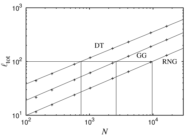
Figure 10: The scaling behavior of the total edge length $\ell_{\rm tot}$ of the RNG, GG and DT. Each data point has been created by averaging over $2000$ instances. In each case the total edge length seems to scale according to $\ell_{\rm tot}\sim N^{0.5}$ for large systems. We used the fit function $\ell_{\rm tot}=a(N+b)^{c}$. By taking the system sizes $N=2304,4096,9216,16384$ into account, we found $a=4.02(2)$, $b=19(5)$, $c=0.4868(4)$ for the DT ($\chi_{\rm red}^{2}$ = 2.44), $a=1.91(1)$, $b=-47(5)$, $c=0.5039(5)$ for the GG ($\chi_{\rm red}^{2}=1.31$) and $a=0.99(1)$, $b=-20(3)$, $c=0.5024(3)$ for RNG ($\chi_{\rm red}^{2}=0.46$).

As a consequence, implementing the topology of the RNG will be the most reasonable, if installing edges is much more expensive than adding further nodes. Certainly, the additional edges of the DT and GG increases the stability, but the benefit of those is small in comparison to the edges which are contained in the RNG anyway.

V Conclusion

In the presented article, the robustness of three types of proximity graphs and a particular geometric random graph (see Sec. II), i.e. their ability to function well even if they are subject to random failures and targeted attacks, was put under scrutiny. For this purpose we generated instances of the considered graph types and successively removed nodes according to three different node removal strategies (see Sec. III). Once the fraction of removed nodes exceeds a certain threshold (characteristic for the particular graph type and node deletion scheme), the underlying graph instance decomposes into many small clusters. Using standard observables from percolation theory (see Sec. IV.2), the critical node removal thresholds were determined for the different graph types and deletion strategies, see Tab. 1. Therein, so as to yield maximally justifiable results through numerical redundancy, we considered various observables to estimate the critical points and exponents. In order of increasing severity, these strategies have an intuitive order: a random node removal mechanism, equivalent to ordinary random percolation, is less severe than a degree-based node removal strategy which takes into account particular node-related local details (i.e. the node-degrees) to optimize the order of node removals during the fragmentation procedure. As evident from Tab. 1, both removal schemes result in finite critical points. The latter strategy is again less severe than the centrality-based node removal mechanism, which takes into account global information (i.e. the set of shortest paths that connect all pairs of nodes) which is used to impose a maximally efficient structural damage by preferentially removing nodes with maximal betweenness centrality (i.e. the most relevant nodes). As evident from Tab. 1 and the discussion in Sec. IV.2, the latter node removal scheme requires to delete only a negligible amount of nodes until the graph decomposes into small clusters. A peculiar result are the fragmentation thresholds related to the random failure and degree-based node removal for the MR geometric graph. As discussed in Sec. IV.2 we cannot rule out that the estimates for both critical points agree within error-bars. This might be attributed to the extensive overlap of the individual node-neighborhoods within the range of the underlying “connectivity radius”. Hence, due to the high number of redundant node-to-node paths which easily allow to compensate for deleted nodes, the effect caused by the removal of a randomly chosen node does not differ much from the effect caused by the removal of a node with a particularly large degree.

For a given node removal strategy, the sequence of critical points for the sub-graph hierarchy ${\rm RNG}\subset{\rm GG}\subset{\rm DT}$ follow the commonly accepted belief that the percolation threshold (or here: the fragmentation threshold) is a non decreasing function of the average degree. This is in full accord with the containment principle due to Fisher Fisher (1961), stating that if $G^{\prime}$ is a sub-graph of $G$, then it holds that $p_{c}^{G^{\prime}}\leq p_{c}^{G}$ for both, bond and site percolation.

Finally, we considered the backup capacity, which is the largest betweenness-centrality increment of the nodes (or edges) after removing the most important node (or edge) beforehand, for the different graph types. Thus, via sufficient backup a graph is made $N-1$ resilient. Regarding the three studied proximity graph ensembles, it turned out that the DT is the most cost efficient one assuming that the backup investments are dominated by improving the nodes. On the other hand, if one has to backup the edges, the more cost efficient one will be either DT or GG, depending on whether the investment depends mainly on the number or on the length of the edges.

For further studies, it would be very interesting to evaluate these simple spatial planar ensembles in the context of more complex transportation networks, like for steady state power grids in the power-flow approximation, Kundur et al. (1994) or for networks of truly dynamically coupled oscillators as for Kurmatoto-like modelsFilatrella et al. (2008); Rohden et al. (2012); Witthaut and Timme (20).