The recurrence time in quantum mechanics

Abstract

Generic quantum systems –as much as their classical counterparts– pass arbitrarily close to their initial state after sufficiently long time. Here we provide an essentially exact computation of such recurrence times for generic non-integrable quantum models. The result is a universal function which depends on just two parameters, an energy scale and the effective dimension of the system. As a by-product we prove that the density of orthogonalization times is zero if at least nine levels are populated and connections with the quantum speed limit are discussed. We also extend our results to integrable, quasi-free fermions. For generic systems the recurrence time is generally doubly exponential in the system volume whereas for the integrable case the dependence is only exponential. The recurrence time can be decreased by several orders of magnitude by performing a small quench close to a quantum critical point. This setup may lead to the experimental observation of such fast recurrences.

I Introduction

The idea that the world will repeat itself after some time is an ancient one and appears in many philosophies and cultures. Babylonians called the Great Year the time needed for the planets to return to their initial conditions Cagni (1977); Marinus van der Sluijs (2005) . However it was only in the end of the XIX century that Henri Poincaré rigorously proved the existence of a recurrence time for a certain description of reality Poincaré (1890). The beauty and the power of Poincaré’s result lie in its simplicity and in its wide range of applicability. The only hypotheses of Poincaré recurrence theorem are that 1) the (phase) space available to the dynamics is bounded in volume; and 2) the dynamical flow $g^{t}$ preserves the volumes . Under such hypotheses the system returns arbitrarily close to its initial conditions after sufficiently long time. Hypothesis 2) is satisfied if we believe a classical, Hamiltonian, description of the world thanks to Liouville’s theorem. Hypothesis 1) holds true if, for instance, the motion is restricted to a bounded region of space because of conservation of energy Gibbs (1902). Poincaré recurrence theorem has philosophical and counterintuitive implications. For example –if we believe a conservative, classical dynamics– the theorem predicts that, if we let two different gases mix by removing a barrier, there will exist a time where we will see the two gases separate again. Indeed Zermelo used Poincaré result’s to argue that Boltzmann’s formula for the entropy should decrease after some sufficiently long time, thus violating the claim that entropy always increases Zermelo (1896). The reason why we never see the two gases nicely separate back again is due to the astronomically large times needed to observe such recurrences. Poincaré’s argument does not give any indication on how to estimate such recurrence times. In order to do that one must generally have stronger assumptions. The very first estimate of recurrence time has been given by Boltzmann himself in reply to Zermelo’s criticism Boltzmann (1896). Boltzmann estimated that the time needed for a $\mathrm{cm}^{3}$ of gas to go back to its initial state, has of the order of many trillion of digits.

In more recent years the estimation of such Poincaré recurrences became an active research topic belonging to the field of dynamical systems Barreira (2006). The first estimation of return times appeared in Hemmer et al. (1958) for a system of harmonic oscillators. More precisely in Ref. Hemmer et al. (1958) the average recurrence has been computed. It is defined by $T_{R}=\lim_{r\to\infty}t_{r}/r,$ where $t_{r}$ is the location of the $r$-th recurrence. As noted by Kac in Kac (1959), the result of Ref. Hemmer et al. (1958) can be obtained almost immediately thanks to the following formula of Smoluchowski, valid for a discrete evolution,

$$T_{R}=\tau\frac{\mu(S)-\mu(A)}{\mu(A)-\mu(g^{\tau}A\cap A)}.$$ (1)

The above formula gives the average time taken to return in set $A$ given that we started from a point of the set. In Eq. (1) $\mu(S)$ is the (finite) invariant measure of the total available phase space and $g^{\tau}$ is the mapping advancing one unit of time $\tau$ (see e.g. Arnold (1978)). The result for continuous evolution is obtained taking the limit $\tau\to 0$. Eq. (1) can readily be applied to a classical integrable system. The assumption of finiteness of the available phase space (more precisely the manifold is assumed to be compact and simply connected), implies that the motion takes place on a $N$ dimensional torus $\mathbb{T}^{N}=\{(\phi_{1},\ldots,\phi_{N})\mod 2\pi\}$, where $N$ is the number of degrees of freedom Arnold (1989). The map $g^{t}$ is given by $g^{t}\boldsymbol{\phi}=(\phi_{1}+\omega_{1}t,\ldots,\phi_{N}+\omega_{N}t)$. If the frequencies $\{\omega_{i}\}$ are rationally independent (RI, i.e. linearly independent over the field of the rationals), time averages are equivalent to phase space averages on the torus and Eq. (1) applies. In this case, if $A$ is taken to be the angular interval $(\Delta\phi_{1},\ldots,\Delta\phi_{N})$, Eq. (1) gives, after taking the $\tau\to 0$ limit,

$$T_{R}=\frac{\left(\prod_{j=1}^{N}\frac{2\pi}{\Delta\phi_{j}}-1\right)}{\sum_{j=1}^{N}\frac{\omega_{j}}{\Delta\phi_{j}}}.$$ (2)

For example, taking for simplicity $\Delta\phi_{j}=\epsilon$ we obtain $T_{R}\simeq\epsilon e^{\ln(2\pi/\epsilon)N}/\sum_{j=1}^{N}\omega_{j}$.

We know however reality is ultimately quantum. Does a recurrence theorem applies also to the quantum world? That this is the case was shown in Ref. Bocchieri and Loinger (1957) but no actual estimate of recurrence time was given. Some approximate estimates for some specific initial states where given in Peres (1982); Bhattacharyya and Mukherjee (1986). In this paper we solve this problem in an essentially exact way.

Let’s assume then, from here on, that the world evolves according to Schrödinger equation and that, for simplicity, the initial state is pure. For the time being we assume that the system’s Hamiltonian $H$ has purely discrete spectrum. This is a crucial assumption on which we will come back (and weaken it) later. Then $H=\sum_{n}E_{n}\Pi_{n}$ with orthogonal projectors $\Pi_{n}$ and let $|\psi\rangle=|\psi(0)\rangle$ the state of the system at $t=0$. We define $|n\rangle=\Pi_{n}|\psi\rangle/\left\|\Pi_{n}|\psi\rangle\right\|$. The state at time $t$ is then $|\psi(t)\rangle=e^{-itH}|\psi\rangle=\sum_{n}\left\|\Pi_{n}|\psi\rangle\right\|e^{-itE_{n}}|n\rangle$ . As time goes by $|\psi(t)\rangle$ spans a $d$ dimensional torus ($d$, possibly infinite, is the number of non-zero $\left\|\Pi_{n}|\psi\rangle\right\|$) with radii $\left\|\Pi_{n}|\psi\rangle\right\|$ and angular frequencies $E_{n}$. If the energies $E_{n}$ are rationally independent (which is natural to assume) the torus is filled uniformly as time goes by. It is tempting then to try to recycle the classical result and use Eq. (2) to estimate the recurrence time in the quantum case. The problem with that is that the distance of points on the torus does not imply any physical distance between states. For example states $|n\rangle$ with large amplitudes $\left\|\Pi_{n}|\psi\rangle\right\|$ should count more than states with small amplitudes. A natural distance between $|\psi(t)\rangle$ and $|\psi\rangle$, instead, is encoded in the fidelity

$$\mathcal{F}(t)=\left|\langle\psi|\psi(t)\rangle\right|^{2}.$$ (3)

The quantity in Eq. (3) is also known under different names such as survival probabilities or Loschmidt echo, and it has been studied in various contexts such as quantum chaos, the theory of fermi edge singularities, equilibration and decoherence Gorin et al. (2006); Schotte and Schotte (1969); Silva (2008); Campos Venuti (2015); Quan et al. (2006). The statistical properties of $\mathcal{F}(t)$ when $t$ is seen as a uniform random variable on the infinite half-line have been investigated in a series of works Campos Venuti and Zanardi (2010a, b, 2013, 2014, 2015); Campos Venuti (2015). If the spectrum of $H$ is discrete, $\mathcal{F}(t)$ is an almost periodic function Besicovitch (1954) and $\mathcal{F}(t)$ evolves indefinitely without ever converging to a limit as $t\to\infty$. Conversely if the spectrum is purely continuous (or if only this part of the spectrum is populated) $\lim_{t\to\infty}\mathcal{F}(t)=0$ essentially because of the Riemann–Lebesgue lemma. In this situation the system does not return close to its initial state and actually becomes orthogonal to it for long times . Hence only if there is a discrete spectrum, and if the corresponding probabilities $p_{n}=\left\|\Pi_{n}|\psi\rangle\right\|^{2}$ are non-zero, the system has a chance to return close to its initial state. We henceforth set ourself in this situation. In this case, typically, $\mathcal{F}(t)$ start from its maximum one at $t=0,$ drops to an average value $\overline{\mathcal{F}}$ in a time that may well be called equilibration time Campos Venuti and Zanardi (2010a); Campos Venuti et al. (2013), and starts oscillating around this value (see Fig. 1 for a typical plot). We are interested in estimating the time $\mathcal{F}(t)$ will go back to a value $u\in[0,1]$ possibly (but not necessarily) close to one. Let us proceed as follows. We call $t_{n}$ the $n$-th solution of the equation $\mathcal{F}(t)=u$ on the half-line $t\geq 0$ starting from the left. We define the (average) recurrence time as $T_{R}(u)=\lim_{n\to\infty}t_{n}/n$. This number clearly does not need to coincide with, for instance the first recurrence, but it’s essentially the only quantity that makes physical sense in that –as we will show– depends only on a finite number of physically relevant constants. Estimating the exact recurrences $t_{n}$, besides being mathematically almost intractable, is physically meaningless. In fact the exact recurrences $t_{n}$ depend crucially on the energy levels $E_{n}$ which must be known with infinite accuracy Lenstra et al. (1982); Kovács and Tihanyi (2013); Jonckheere et al. (2014). Since the latter seems a rather unphysical presumption we focus on the computation of $T_{R}(u)$.

Our strategy will be the following. First we estimate the number of zeros $N_{T}(u)$ of the equation $\mathcal{F}(t)=u$ in a large segment $[0,T]$ with $T\gg 1$. We will show that, for large $T$, $N_{T}(u)\simeq T\,D(u)$ with a finite density $D(u)$. Then the recurrence time is given by $T_{R}(u)=\lim_{T\to\infty}T/N_{T}(u)=1/D(u)$.

We now show how to compute $D(u)$. Similar techniques have been pioneered by Kac and Rice to study the average number of roots of a random polynomial or time signal Kac (1943); Rice (1944).

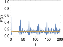
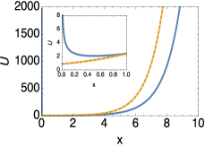
Figure 1: Left panel: typical behavior of the fidelity for a many body system. The system is given by Hamiltonian Eq. (13) with $\kappa=0$ with $L=50$. The horizontal line is the location of the average $\overline{\mathcal{F}}$. The peaks observed at times approximately integer multiple of the system size are revivals discussed in Campos Venuti and Zanardi (2010a). Right panel: universal function $\mathcal{U}(x)=(\sqrt{\pi}/2)e^{x}/\sqrt{x}$. $\mathcal{U}(x)$ has essentially three regimes: for $x\ll 1$, $\mathcal{U}(x)\sim 1/\sqrt{x}$, for $x=O(1)$, $\mathcal{U}(x)\sim O(1)$ whereas for $x\gg 1$, $\mathcal{U}(x)\sim e^{x}$ (dashed line).

II Non-integrable case

We assume here the the Hamiltonian $H$ has pure discrete spectrum and will consider generalizations later. This condition plays an analogous role as the requirement of a compact phase space for the classical case. The Hamiltonian has then the following spectral decomposition $H=\sum_{n}E_{n}\Pi_{n}$ with eigen-projectors $\Pi_{n}$.

The number of zeros of the function $\mathcal{F}(t)-u$ in the interval $[0,T]$, is given by the following formula

$$N_{T}(u)=\int_{0}^{T}\delta(\mathcal{F}(t)-u)\left|\mathcal{F}^{\prime}(t)\right|dt,$$ (4)

as can be checked by a change of variable (and with $\mathcal{F}^{\prime}(t)=d\mathcal{F}(t)/dt$). For large $T$ we can use $N_{T}(u)=TD(u)+O(T^{0})$ where the density is given by $D(u)=\lim_{T\to\infty}T^{-1}\int_{0}^{T}\delta(\mathcal{F}(t)-u)\left|\mathcal{F}^{\prime}(t)\right|dt$ provided $D(u)$ is finite. The density can then be computed with

$$D(u)=\int df^{\prime}\left|f^{\prime}\right|P_{\mathcal{F},\mathcal{F}^{\prime}}(u,f^{\prime})$$ (5)

where $P_{\mathcal{F},\mathcal{F}^{\prime}}(f,f^{\prime}):=\overline{\delta(\mathcal{F}(t)-f)\delta(\mathcal{F}^{\prime}(t)-f^{\prime})}$ is the joint probability distribution of $\mathcal{F}$ and $\mathcal{F}^{\prime}$, and overline indicates infinite time average, i.e. $\overline{a(t)}:=\lim_{T\to\infty}T^{-1}\int_{0}^{T}a(t)dt$. For the next step we assume that the energies $E_{n}$ are rationally independent, i.e. linearly independent over the field of rationals. This is a very reasonable assumptions for generic non-integrable system. Thanks to rational independence we can express time averages as phase space averages over a large multi-dimensional torus Arnold (1989). The steps are detailed in the Appendix B. The main ingredient is given by the fact a certain distribution related to $P_{\mathcal{F},\mathcal{F}^{\prime}}$, becomes Gaussian in the limit of large dimensionality.

The final result for the recurrence time is surprisingly simple

$$T_{R}(u)=\frac{\sqrt{\pi}}{2}\frac{1}{\Delta E}\sqrt{\frac{\overline{\mathcal{F}}}{u}}e^{u/\overline{\mathcal{F}}},$$ (6)

where $\overline{\mathcal{F}}=\sum_{j}p_{j}^{2}$ and $\Delta E^{2}$ is the variance of the energy $\{E_{n}\}$ with respect to the ensemble $\nu_{n}=p_{n}^{2}/\sum_{n}p_{n}^{2}$, i.e. $\Delta E^{2}=[\sum_{j}p_{j}^{2}E_{j}^{2}/\overline{\mathcal{F}}-(\sum_{j}p_{j}^{2}E_{j}/\overline{\mathcal{F}})^{2}]$. The factor $1/\Delta E$ is essentially needed to reproduce the correct dimensionality whereas the main dependence is through a universal function of $x=u/\overline{\mathcal{F}}$, $\mathcal{U}(x)=(\sqrt{\pi}/2)e^{x}/\sqrt{x}$ (see Fig. 1 right panel). Since, forgetting the size dependence, $\Delta E\sim J$ where $J$ is some energy scale of $H$, a good approximation of Eq. (6) is given by $T_{R}\sim J^{-1}\sqrt{\overline{\mathcal{F}}/u}e^{u/\overline{\mathcal{F}}}$. Several considerations can be drawn on the basis of Eq. (6):

1) For macroscopic systems the recurrence time is, in general, doubly exponential in the system’s volume. Indeed, in the typical situation, the average fidelity is exponentially small in the system volume, $\overline{\mathcal{F}}\sim e^{-\alpha V}$ with $\alpha$ positive constant (see e.g. Campos Venuti and Zanardi (2013)) . Sufficient conditions are i) the Hamiltonian is local and extensive, meaning $H$ can be written as $H=\sum_{x}h(x)$, with $h(x)$ locally supported operators; together with ii) the initial state is exponentially clustering, i.e. the state $\langle\bullet\rangle$ satisfies $\langle h(x)h(y)\rangle-\langle h(x)\rangle\langle h(y)\rangle=O\left(e^{-|x-y|/\xi}\right)$. Hence, under these very general conditions, one has readily $T_{R}(u)\sim J^{-1}e^{ue^{\alpha V}}$ (for $u\gg\overline{\mathcal{F}}$).

2) It is tempting to relate the recurrence time to the concept of entropy. With the aid of the equilibrium state $\overline{\rho}:=\overline{|\psi(t)\rangle\langle\psi(t)|}$ one can write $H_{2}(\overline{\rho})=-\ln\overline{\mathcal{F}}$, the 2-Rényi entropy of $\overline{\rho}$. Recall the entropy inequality $H_{2}(\overline{\rho})\leq S(\overline{\rho})$ where $S$ is the Von Neumann entropy of $\overline{\rho}$, $S(\overline{\rho})=-\mathrm{tr}\overline{\rho}\ln\overline{\rho}$. The inequality becomes tight in the limit of totally mixed $\overline{\rho}$, i.e. when $\overline{\mathcal{F}}$ is small. Since, as we have shown, typically $\overline{\mathcal{F}}\sim e^{-\alpha V}$ a possible proxy to the recurrence time (for $u\gg\overline{\mathcal{F}}$) is given by (omitting pre-factors) $T_{R}\sim J^{-1}e^{ue^{S}}$, a formula sometimes found in the literature (see e.g., Ref. Page (1994)).

3) Equation (6) and its inverse $D(u)=1/T_{R}(u)$ should be handled with care at the extrema $u=0$ or $u=1$. For example Eq. (6) predicts a finite density of exact recurrences ($u=1$) but a zero density of orthogonalization times (i.e. times for which $\mathcal{F}(t)=0$). This is quite surprising given the fact that typically $\mathcal{F}(t)$ spends much of the time close to its average $\overline{\mathcal{F}}$ which in turn is very close to zero. One can ask wether these results are correct or are a consequence of the Gaussian approximation used to derive (6). The tiny density of exact recurrences (for $u=1$) predicted by Eq. (6), is indeed a consequence of the Gaussian approximation. In fact, for rationally independent energies the only solution of $\mathcal{F}(t)=1$ is at $t=0$ (see Appendix C for a proof). Instead, using this approach without the Gaussian approximation we have been able to prove that indeed the density of orthogonalization times is zero (see Appendix B), provided at least nine energy levels are populated and the energies are RI.

4) For $u$ close to 1 the roots of $\mathcal{F}(t)=u$ are very close to a maximum of $\mathcal{F}(t)$, hence they must come in close pairs. This means that essentially, for $u\approx 1$ a more precise estimate of the recurrence time is given by $2T_{R}(u)$. More importantly, on the basis of numerical simulations, we observed that, for $u$ close to one, the solutions of $\mathcal{F}(t)=u$ come in very narrow spikes. In other words, even if a time $t$ exists for which the system returns close to its initial state, at a later time $t+\Delta t$, with $\Delta t$ very small, the system is likely to differ strongly form the initial state, and be nearly orthogonal to it if $\overline{\mathcal{F}}$ is small.

5) Eq. (6) has been derived assuming a finite number $d$ of non-zero $p_{j}$. Nothing really dangerous happens taking the limit $d\to\infty$, provided the spectrum stays discrete and numerable and $\Delta E$ and $\overline{\mathcal{F}}$ stay finite and non-zero ($\overline{\mathcal{F}}$ is finite because $\overline{\mathcal{F}}\leq\langle\psi|\psi\rangle=1$). In fact also in this case $\mathcal{F}(t)$ is an almost periodic function. In a more general situation $H$ can also have a continuous spectrum. The characteristic function $\chi(t)=\langle\psi|\psi(t)\rangle$ can then be written as

$$\chi(t)=\sum_{n}p_{n}e^{-iE_{n}t}+\int g(\epsilon)e^{-it\epsilon}d\epsilon,$$ (7)

where the positive function $g(\epsilon)$ (this is the continuous part of the projected density of states, PDOS, $\langle\psi|\delta(H-\epsilon)|\psi\rangle$) has support on the continuous spectrum. If $g(\epsilon)d\epsilon$ is absolutely continuous, the Riemann-Lebesgue lemma guarantees that $\lim_{t\to\infty}\int g(\epsilon)e^{-it\epsilon}d\epsilon=0$ . Hence, in this case, the second term of Eq. (7) contributes at most a finite number of zeroes. A similar argument with small modifications, works for the fidelity $\left|\chi(t)\right|^{2}$. Hence we deduce that Eq. (6) works also in this more general setting with the caveat that the $p_{n}$s refer only to the discrete spectrum and one may not have $\sum_{n}p_{n}=1$. Note that Eq. (6) should be utilized with $u\in(0,M)$ with $M=\sum_{n}p_{n}<1$. Moreover the Gaussian approximation employed may become worse if the missing term $\int g(\epsilon)d\epsilon$ becomes a sensible fraction of $1.$

The above results inspire some connections for the debate around the quantum speed limit if we consider Eq. (6) for $u\ll 1$ Mandelstam and Tamm (1945); Margolus and Levitin (1998); Giovannetti et al. (2003a, b). In some situations (for example to estimate the computational power of the ultimate laptop or the universe Lloyd (2000, 2002)) one is interested in counting the number of total distinct (i.e., orthogonal) states that a “system can pass through in a given period of time” Margolus and Levitin (1998). Calling $T_{QSL}$ the minimum time it takes for a system to go to an orthogonal state, it is known that $T_{QSL}\geq(\pi/2)/(\langle H\rangle-E_{0})$. Accordingly, in Ref. Margolus and Levitin (1998), it was estimated that the maximum number of states, $N_{\mathrm{max}}$, a system can pass through in a time interval $T$, is given by $N_{\mathrm{max}}=(2/\pi)(\langle H\rangle-E_{0})T$. However, in this situation where the initial state is specified, there is no need to compute $N_{\mathrm{max}}$, but rather $N_{T}(u)$ is the number we are after. Now, if $T$ is sufficiently large, the number of times the state returns at fidelity $u$, is precisely given by $N_{T}(u)\simeq T/T_{R}=T\Delta E/\mathcal{U}(u/\overline{\mathcal{F}})$. Some considerations are in order. i) Exactly at $u=0$, as discussed in 3), one has actually $N_{T}(u)=o(T)$ (i.e. $\lim_{T\to\infty}N(u)/T=0$) for RI energies when at least nine levels are populated; ii) The estimate $N_{\mathrm{max}}$ of Ref. Margolus and Levitin (1998) qualitatively agrees with our $N(u)$ in the region where exponential and square root terms are ineffective, i.e. for $u/\overline{\mathcal{F}}\sim 1$. In fact in this region we have $N_{T}(u)\sim T\Delta E$. Note that $u/\overline{\mathcal{F}}\sim 1$ is likely the region where one would want to use these results, since, as we have seen, typically $\overline{\mathcal{F}}$ is very small. However the relevant energy scale is not $(\langle H\rangle-E_{0})$, (and not even the standard deviation $\sqrt{\langle H^{2}\rangle-\langle H\rangle^{2}}$), but rather the standard deviation $\Delta E$ computed with the “squared” distribution $\nu_{n}=p_{n}^{2}/\overline{\mathcal{F}}$.

III Integrable case

The result Eq. (6) is valid assuming rational independence of the many-body spectrum. This condition is massively violated for quasi-free integrable models whose Hamiltonian is quadratic in creation and annihilation Fermi/Bose operator. It is an interesting question per se to compare typical timescale of integrable systems with non-integrable ones . We consider hence a quasi-free system of fermions where the Hamiltonian $H$ is bilinear in $c_{i},\,c_{i}^{\dagger}$ ($c_{j}$ Fermi annihilation operators) and the initial state is Gaussian (i.e. satisfies Wick’s theorem). For simplicity we consider a one-dimensional geometry and assume that the fidelity can be written in the form

$$\mathcal{F}(t)=\prod_{k}\left[1-\alpha_{k}\sin^{2}(t\epsilon_{k}/2)\right],$$ (8)

where $\{\epsilon_{k}\}$ is the one-particle spectrum of $H$, $k$ is a quasi-momentum label, i.e. $k=\pi(2n+1)/L$, with $n=0,1,\ldots,L$, $L$ is the number of sites and $\alpha_{k}\in[0,1]$. This is the case for example for quenches of the one dimensional XY model, but can be valid more generally provided the Hamiltonian and the state are translationally invariant. In particular generalization of Eq. (8) to $D$-dimensions is straightforward promoting $k$ to a $D$-dimensional vector in the Brillouin zone.

This is one of the rare cases where the calculation is harder for integrable systems because the need of passing to the one particle space introduces additional complications. For quasi-free systems it is known that the logarithm of the fidelity (instead of the fidelity itself) becomes Gaussian distributed Campos Venuti et al. (2011). It is then natural to consider the variable $Z(t)=\log\mathcal{F}(t)$. We will then estimate the number of zeroes of the equation $\log\mathcal{F}(t)=\ln u$. Proceeding as previously we are now led to consider the joint probability distribution $P_{Z,Z^{\prime}}(z,z^{\prime})=\overline{\delta(Z(t)-z)\delta(Z^{\prime}(t)-z^{\prime})}$. For large $L$, $P_{Z,Z^{\prime}}$ becomes Gaussian and using Eq. (5) one obtains

$$T_{R}=\frac{\pi\sigma_{Z}}{\sigma_{Z^{\prime}}}\exp\left[(\ln u-\overline{\ln\mathcal{F}})^{2}/(2\sigma_{Z}^{2})\right],$$ (9)

with coefficients given by

$$\overline{\ln\mathcal{F}} = \sum_{k}\overline{z_{k}}$$ (10)

$$\sigma_{Z}^{2} = \sum_{k}\left[\overline{(z_{k})^{2}}-(\overline{z_{k}})^{2}\right]$$ (11)

$$\sigma_{Z^{\prime}}^{2} = \sum_{k}\overline{(z^{\prime}_{k})^{2}},$$ (12)

and $\overline{z_{k}},\,\overline{(z_{k})^{2}},\,\overline{(z^{\prime}_{k})^{2}}$ are smooth, bounded, function of $\alpha_{k},\epsilon_{k}$. Some remarks are in order.

1) The sum over $k$ in Eqns. (10)-(12), runs over an extensive number of terms. Accordingly (since the summand functions are bounded) we conclude that both $\overline{\ln\mathcal{F}}$ and $\sigma_{F}^{2}$ are extensive quantity. This implies that the recurrence time for quasi-free fermions is only exponentially large in the system volume.

2) The behavior at the border $u\to 0,1$ must be handled with particular care. Similarly as in the non-integrable case, Eq. (9) predicts a finite density of exact recurrences times and a zero density of orthogonalization times. The small, finite density of exact recurrences predicted by Eq. (9) at $u=1$, is a consequence of the Gaussian approximation. In fact a similar argument as for the non-integrable case shows that, if all $\alpha_{k}$ are positive, $\mathcal{F}(t)=1$ only at $t=0$.

3) The exponential vs. the double exponential dependence of the recurrence time with the system’s volume may suggest that $T_{R}$ may serve as a detector of integrability. However, any (no matter how small) non-integrable perturbation of an integrable model will result (with probability one) in a rationally independent many-body spectrum and consequently a $T_{R}$ given by Eq. (6). As a consequence $T_{R}$ will be discontinuous at the integrable point. A similar behavior has been observed for the temporal variances Campos Venuti and Zanardi (2013).

IV Fast recurrences

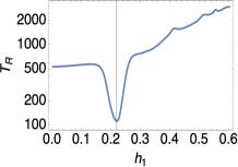
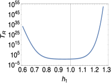
Figure 2: Recurrence time in small quench experiments near criticality. The system is initialized in the ground state of Hamiltonian (13) with parameter $\kappa_{1},\,h_{1}$ and then let evolve with the same Hamiltonian with parameters $\kappa_{2},\,h_{2}$. Left panel: non-integrable case with $\kappa_{1}=\kappa_{2}=0.4$. Other parameters are $L=12,\,,h_{2}=h_{1}+\delta h,\delta h=0.03,u=0.98$. The recurrence time is given by Eq. (6). The vertical line signals the estimated critical point $h_{c}=0.218$. Right panel: integrable case with $\kappa_{1}=\kappa_{2}=0$. Other parameters are $L=12,\,,h_{2}=h_{1}+\delta h,\delta h=0.03,u=0.98$. The recurrence time is given by Eq. (9). The vertical line signals the critical point $h_{c}=1$.

The double exponential growth of the recurrence time with the system’s volume, poses serious questions on the possibility of observing recurrence times in practical situations. On the other hand in some cases it may be possible to prepare the initial state such that $p_{n}=0$ but for a few terms. Rabi oscillations may be seen as a limiting case of this situation. Another possibility is provided by a small quench experiment. In a quench experiment the system is initialized in the ground state of the system’s Hamiltonian with certain parameters $\lambda_{1}$. The parameters are then suddenly changed and the system is evolved with parameters $\lambda_{2}=\lambda_{1}+\delta\lambda$. Whereas a general perturbation results in roughly as many excitations as the Hilbert’s space dimension, for sufficiently small quench amplitude $\delta\lambda$, the number of excited quasi-particles is proportional to the system’s volume. A sufficient condition for small quench is given by $\left|\delta\lambda\right|\ll L^{-D/2}$ where $L$ is the linear system’s size and the $D$ spatial dimensionality. As a consequence the system evolves effectively in a small Hilbert space whose dimension is roughly given by $1/\overline{\mathcal{F}}$ Linden et al. (2009) and the recurrence time can be diminished by several order of magnitudes. In fact one has $\overline{\mathcal{F}}\simeq 1-\delta\lambda^{2}cV$ ($c$ positive constant $O(1)$) and hence $T_{R}\simeq e^{u\delta\lambda^{2}cV}$. However a further reduction is possible. If the system is close to a critical point, the effective dimension $1/\overline{\mathcal{F}}$ is brought down to $2-3$ and $T_{R}$ becomes roughly $J^{-1}O(1)$. A sufficient condition for small quench becomes in this case $\left|\delta\lambda\right|\ll L^{-1/\nu}$ where $\nu$ is the critical exponent of the correlation length $\xi$ Campos Venuti (2015), whereas the quasi-critical regime is defined by by $\xi(\lambda_{i})\gg L$. In this regime the recurrence time is roughly size independent and may well become observable.

To illustrate these effects we show numerical results for the one-dimensional Ising model in transverse field with additional next nearest neighbor interaction. The, so called, TAM Hamiltonian, is given by

$$H=-\sum_{i=1}^{L}\left(\sigma_{i}^{x}\sigma_{i+1}^{x}-\kappa\sigma_{i}^{x}\sigma_{i+2}^{x}+h\sigma_{i}^{z}\right),$$ (13)

with periodic boundary conditions ($\sigma_{L+i}^{x}=\sigma_{i}^{x}$). Hamiltonian Eq. (13) is integrable at $\kappa=0$ and non-integrable for all $\kappa\neq 0$ (see e.g. Beccaria et al. (2006, 2007)). The parameters are initialized to $\kappa_{1},\,h_{1}$ and then suddenly changed to $\kappa_{2},\,h_{2}$. We first illustrate the (double exponential) reduction in recurrence time for a small quench close to a non-integrable critical point. For small frustration $\kappa\leq 1/2$, there is a transition from a ferromagnetic to a paramagnetic phase increasing the external field $h$. Numerical simulations using Eq. (6) are shown in Fig. 2 left panel. It is evident the sharp drop close to the quantum critical point.

Similar considerations also apply to the integrable case for which we set $\kappa=0$ in Eq. (13). In this case the fidelity is precisely given by Eq. (8) . Again one observes a drop (albeit less sharp) close to the quantum critical point Fig. 2 right panel.

V Conclusions

We provided essentially exact formulas for the average recurrence time in quantum systems both for general non-integrable and integrable models. This is the –average– time a system takes to get back to the initial state up to an error $1-u$ in fidelity. We have shown that, in the typical case, recurrence times are doubly exponential in $V$, i.e. $T_{R}\sim(\hbar/J)e^{ue^{\alpha V}}$, where $V$ is the dimensionless system’s volume normalized by the volume of the unit cell, $J$ a system’s energy scale and $\alpha$ a positive constant. Most of the time a valid approximation is given by $T_{R}\sim(\hbar/J)e^{ue^{S}}$ where $S$ is the Von Neumann’s entropy of the equilibrium state. For integrable systems instead the recurrence times are down to a simple exponential in $V$.

A possibility to drastically reduce such astronomical recurrence times is to perform a small quench experiment. By this we mean preparing the system in the ground state; slightly change some Hamiltonian parameters, and let the system evolve undisturbed thereafter. In this situation recurrences happen on a time-scale which is only exponential in the volume. Furthermore if the quench is performed close to a quantum critical point recurrence times become roughly size independent. This drastic reduction opens up the possibility to experimentally observe such fast recurrences in several nearly isolated quantum platforms. In particular ion traps with order of $10$ atoms seems to be particularly suited.

Appendix A Densities of zeroes in the non-integrable case

The fidelity is the modulus square of the characteristic function

$$\chi(t)=\sum_{n}p_{n}e^{-itE_{n}}\,,$$ (14)

with weights $p_{n}=\langle\psi|\Pi_{n}|\psi\rangle$. The investigation of sums of the form Eq. (14) was initiated long ago by Lagrange Lagrange (1781). The study of the variation of perihelion leads to a study of the variation of the argument of such a sum where the number of terms is the number of planets. Here instead we are interested in the behavior of the modulus.

We now write $\chi=X+iY$ such that $\mathcal{F}=X^{2}+Y^{2}$ and $\mathcal{F}^{\prime}=2XX^{\prime}+2YY^{\prime}$ with

$$X = \sum_{j}p_{j}\cos(E_{j}t)$$ (15)

$$Y = \sum_{j}p_{j}\sin(E_{j}t)$$ (16)

$$X^{\prime} = -\sum_{j}p_{j}E_{j}\sin(E_{j}t)$$ (17)

$$Y^{\prime} = \sum_{j}p_{j}E_{j}\cos(E_{j}t).$$ (18)

Note that, to avoid an overburdened notation, we use the same latter to indicate both a function of time (e.g. $X(t)$) and a random variable ($X$) obtained convoluting $t$ seen as a random variable with uniform distribution in $[0,T]$ and taking the limit $T\to\infty$. We also use the compact notation $\boldsymbol{X}=(X,Y,X^{\prime},Y^{\prime})$ and $\boldsymbol{x}=(x,y,x^{\prime},y^{\prime})$. With the help of the joint distribution function $P_{\boldsymbol{X}}(\boldsymbol{x})$, the density of zeros can be written as

$$D(u)=\int dxdydx^{\prime}dy^{\prime}\,\delta(u-x^{2}-y^{2})2\left|xx^{\prime}+yy^{\prime}\right|\times\\ P_{\boldsymbol{X}}(x,y,x^{\prime},y^{\prime}).$$ (19)

From equations (15)–(18) and the RI assumption it follows that $\boldsymbol{X}$ is a sum of independent random vectors. Indeed the characteristic function of $\boldsymbol{X}$ ($\boldsymbol{k}=(\xi,\eta,\xi^{\prime},\eta^{\prime})$) is

$$\varphi_{\boldsymbol{X}}(\boldsymbol{k}) =\overline{e^{i\boldsymbol{k}\cdot\boldsymbol{X}}}$$ (20)

$$=\prod_{j}\int\frac{d\vartheta_{j}}{2\pi}\exp[iA_{j}\cos(\vartheta_{j})+iB_{j}\sin(\vartheta_{j})]$$ (21)

$$=\prod_{j}J_{0}(\sqrt{A_{j}^{2}+B_{j}^{2}})=e^{-\sum_{j}(A_{j}^{2}+B_{j}^{2})/4+O(\boldsymbol{k}^{4})},$$ (22)

where $J_{0}$ is the Bessel function of the first kind and with $A_{j}=p_{j}(\xi+E_{j}\eta^{\prime})$ and $B_{j}=p_{j}(\eta-E_{j}\xi^{\prime})$. Using Eq. (22) it may be possible to rigorously prove normality of (a properly rescaled version of) $\boldsymbol{X}$ under some conditions using the central limit theorem for triangular arrays. This would require to have a well defined family of models parametrized, for example, by the size. This is not always possible and so it will not be further pursued here. Discarding the small, $O(\boldsymbol{k}^{4})$, term in Eq. (22) we realize that $P_{\boldsymbol{X}}(\boldsymbol{x})$ has approximately the following Gaussian form

$$P_{\boldsymbol{X}}(\boldsymbol{x}) = \frac{e^{-\boldsymbol{x}^{T}\Sigma^{-1}\boldsymbol{x}/2}}{\pi^{2}\Delta},$$ (23)

with inverse correlation matrix given by

$$\Sigma^{-1}=\frac{2}{(DF-E^{2})}\left(\begin{array}[]{cccc}F&0&0&-E\\ 0&F&E&0\\ 0&E&D&0\\ -E&0&0&D\end{array}\right),$$ (24)

having defined

$$D = \sum_{j}p_{j}^{2}=\overline{\mathcal{F}}$$ (25)

$$E = \sum_{j}p_{j}^{2}E_{j}$$ (26)

$$F = \sum_{j}p_{j}^{2}E_{j}^{2}\,.$$ (27)

The positivity of the matrix $\Sigma$ reduces to $\Delta:=DF-E^{2}\geq 0$ which can be easily proved using Cauchy-Schwarz inequality with the vectors $\boldsymbol{v}=(p_{1},p_{2},\ldots)$ and $\boldsymbol{w}=(E_{1}p_{1},\omega_{2}p_{2},\ldots)$ (under assumption of convergence) $\left|\boldsymbol{v}\cdot\boldsymbol{w}\right|^{2}\leq\left\|\boldsymbol{v}\right\|^{2}\left\|\boldsymbol{w}\right\|^{2}$.

We now pass to polar coordinates $\left(x,y\right)=\rho_{1}\left(\cos\vartheta_{1},\sin\vartheta_{1}\right)$ and $\left(x^{\prime},y^{\prime}\right)=\rho_{2}\left(\cos\vartheta_{2},\sin\vartheta_{2}\right)$. The density of zeroes becomes

$$D(u) =\int dxdydx^{\prime}dy^{\prime}\,\delta(u-x^{2}-y^{2})2\left|xx^{\prime}+yy^{\prime}\right|$$

$$\times P_{\boldsymbol{X}}(x,y,x^{\prime},y^{\prime})$$ (28)

$$=\int_{0}^{\infty}\!\!d\rho_{1}\int_{0}^{\infty}\!\!d\rho_{2}\,(\rho_{1}\rho_{2})^{2}\delta(u-\rho_{1}^{2})P_{\boldsymbol{X}}(\boldsymbol{\rho},\boldsymbol{\vartheta})$$ (29)

$$\times\int_{0}^{2\pi}\!\!d\vartheta_{1}\int_{0}^{2\pi}\!\!d\vartheta_{2}\,2\left|\cos(\vartheta_{1}-\vartheta_{2}))\right|.$$ (30)

Using the Gaussian approximation Eq. (23), the integration over $\rho_{1}$ is trivial and the result is

$$D(u)=\sqrt{u}\int_{0}^{\infty}\!\!d\rho_{2}\rho_{2}^{2}\int_{0}^{2\pi}\!\!d\vartheta_{1}\int_{0}^{2\pi}\!\!d\vartheta_{2}\\ \times\left|\cos(\vartheta_{1}-\vartheta_{2})\right|\tilde{P}(\rho_{2},\vartheta_{1},\vartheta_{2})$$ (31)

where

$$\tilde{P}(\rho_{2},\vartheta_{1},\vartheta_{2})=e^{-\alpha\rho_{2}^{2}-\beta\sin(\vartheta_{1}-\vartheta_{2})\rho_{2}-\gamma}\frac{1}{\pi^{2}\Delta}$$

and the coefficients are fixed by

$$\left.\boldsymbol{x}\Sigma^{-1}\boldsymbol{x}/2\right|_{\rho_{1}=\sqrt{u}}=\\ \frac{D\rho_{2}^{2}+2E\sqrt{u}\rho_{2}\sin(\vartheta_{1}-\vartheta_{2})+Fu}{DF-E^{2}},$$

and are given by

$$\alpha =\frac{D}{\Delta}$$ (32)

$$\beta =\frac{2E\sqrt{u}}{\Delta}$$ (33)

$$\gamma =\frac{Fu}{\Delta}.$$ (34)

Now the angular integration can be performed

$$\int_{0}^{2\pi}\!\!d\vartheta_{1}\int_{0}^{2\pi}\!\!d\vartheta_{2}\,\left|\cos(\vartheta_{1}-\vartheta_{2})\right|e^{-\beta\rho_{2}\sin(\vartheta_{1}-\vartheta_{2})}\\ =8\pi\frac{\sinh(\beta\rho_{2})}{\beta\rho_{2}}.$$ (35)

The remaining integration over $\rho_{2}$ is Gaussian and the final result is extremely simple

$$D(u)=\frac{2}{\sqrt{\pi}}\frac{\sqrt{u\Delta}}{\overline{\mathcal{F}}^{3/2}}e^{-u/\overline{\mathcal{F}}}.$$ (36)

Using the ensemble $\nu_{n}=p_{n}^{2}/\sum_{n}p_{n}^{2}$, the variance of the energy $\{E_{n}\}$ is $\Delta E^{2}=[\sum_{j}p_{j}^{2}E_{j}^{2}/\overline{\mathcal{F}}-(\sum_{j}p_{j}^{2}E_{j}/\overline{\mathcal{F}})^{2}]=\Delta/\overline{\mathcal{F}}^{2}$ and we obtain

$$D(u)=\frac{2}{\sqrt{\pi}}\Delta E\sqrt{\frac{u}{\overline{\mathcal{F}}}}e^{-u/\overline{\mathcal{F}}},$$ (37)

which, upon remembering that $T_{R}=1/D(u)$, coincides with Eq. (6). The exponential term in Eq. (6) could have been obtained with the following (wrong) argument sometimes used in physics. According to this argument, $T_{R}(u)$, i.e., the average of the solutions of $\mathcal{F}(t)=u$, is approximately estimated by the inverse probability (density) of the event $\mathcal{F}(t)=u$ (time some unknown time-scale $J^{-1}$). The probability density of the fidelity has been computed in Campos Venuti and Zanardi (2010a, 2014) and is given by $P_{\mathcal{F}}(u)=\vartheta(u)\exp(-u/\overline{\mathcal{F}})/\overline{\mathcal{F}}$ ($\vartheta(u)$ Heaviside function). This argument then predicts, $T_{R}(u)\sim J^{-1}\overline{\mathcal{F}}\exp(u/\overline{\mathcal{F}})$ which fails if $u$ is not sufficiently away from zero.

Appendix B Proof of zero density for $u=0$

Throughout this section we assume that only a finite number $d^{\prime}$ of $p_{n}$’s are non-zero. The result (36) predicts a zero density of orthogonalization times, i.e. times for which $\mathcal{F}(t)=0$. It is legitimate to ask weather this holds exactly or is an artifact of the Gaussian approximation used to derive Eq. (36). We then go back to equation (28) in its exact form that we re-write here for clarity

$$D(u) = \sqrt{u}\int_{0}^{\infty}d\rho_{2}\rho_{2}^{2}\int_{0}^{2\pi}d\vartheta_{1}\int_{0}^{2\pi}d\vartheta_{2}\,\left|\cos(\vartheta_{1}-\vartheta_{2})\right|$$ (38)

$$\times P_{\boldsymbol{X}}(\sqrt{u}\cos\vartheta_{1},\sqrt{u}\sin\vartheta_{1}\rho_{2}\cos\vartheta_{2},\rho_{2}\sin\vartheta_{2})$$

$$=: \sqrt{u}R(u)$$

We will show that $R(u)$ is bounded for all $u$, in particular for $u=0$. The result then simply follows from Eq. (38) taking the limit $u\to 0$. Let us analyze the logic. First we show that, by construction, $P_{\boldsymbol{X}}(\boldsymbol{x})$ is compactly supported. Then we prove that $P_{\boldsymbol{X}}(\boldsymbol{x})$ is also bounded thus implying that $R(u)$ is bounded.

Lemma

The function $P_{\boldsymbol{X}}(x,y,x^{\prime},y^{\prime})$ is compactly supported provided $\langle\left|H\right|\rangle$ is finite, more precisely, $P_{\boldsymbol{X}}(x,y,x^{\prime},y^{\prime})=0$ outside the (hyper) rectangle $\left|x\right|,\left|y\right|\leq 1$ and $\left|x^{\prime}\right|,\left|y^{\prime}\right|\leq C=\sum_{j}p_{j}\left|E_{j}\right|=\langle\left|H\right|\rangle$. The latter quantity is certainly finite for the finite dimensional case, physically it can be postulated to grow as the system’s volume.

It is obvious that $P_{\boldsymbol{X}}(x,y,x^{\prime},y^{\prime})=0$ for $\left|x\right|,\left|y\right|>1$. On the other hand $\left|X^{\prime}\right|=\left|-\sum_{j}p_{j}E_{j}\cos(E_{j}t)\right|\leq\sum_{j}p_{j}\left|E_{j}\right|=C$, QED. Now $P_{\boldsymbol{X}}(\boldsymbol{x)}$ is bounded provided the characteristic function (its Fourier transform) $\varphi_{\boldsymbol{X}}(\boldsymbol{k})\in L^{1}(\mathbb{R}^{4}).$ The reminder of this section is devoted to asses the conditions under which $\varphi_{\boldsymbol{X}}(\boldsymbol{k})$ is summable.

Remind the definition of $\varphi_{\boldsymbol{X}}(\boldsymbol{k})$

$$\varphi_{\boldsymbol{X}}(\boldsymbol{k})=\prod_{j=1}^{d^{\prime}}J_{0}(\sqrt{\boldsymbol{k}^{T}M_{j}\boldsymbol{k}})$$ (39)

where $d^{\prime}$ is the number of non-zero $p_{j}$ and

$$M_{j}=p_{j}^{2}\left(\begin{array}[]{cccc}1&0&0&E_{j}\\ 0&1&-E_{j}&0\\ 0&-E_{j}&E_{j}^{2}&0\\ E_{j}&0&0&E_{j}^{2}\end{array}\right).$$ (40)

The matrix $M_{j}$ is hermitian, positive semi-definite, has eigenvalues $0([\times 2]$ and $p_{j}^{2}(1+E_{j}^{2})[\times 2]$ and a null space $V_{j}=\mathrm{span}\left\{\left(E_{j},0,0,-1\right),\left(0,E_{j},1,0\right)\right\}$. The Bessel function is smooth and everywhere bounded and hence so is $\varphi_{\boldsymbol{X}}(\boldsymbol{k})$. To see wether it is summable we must look at its behavior as $\boldsymbol{k}\to\infty$. Remember that, for $x\to\infty$, neglecting an oscillating factor, we have $\left|J_{0}(x)\right|\sim\sqrt{2/\pi}/\sqrt{x}$. Let us fix an $\varepsilon>0$ and define the cylinders (in this picture the planes become lines) $T_{j}=\{\boldsymbol{k}|\boldsymbol{k}M_{j}\boldsymbol{k}\leq\epsilon^{2}\}$. We call “Tubes” the collection (union) of all the $T_{j}$’s. We want to see if and when the following integral is convergent

$$\int_{\mathbb{R}^{4}}\left|\varphi_{\boldsymbol{X}}(\boldsymbol{k})\right|d\boldsymbol{k}=\\ \int_{\mathbb{R}^{4}\backslash\mathrm{Tubes}}\left|\varphi_{\boldsymbol{X}}(\boldsymbol{k})\right|d\boldsymbol{k}+\int_{\mathrm{Tubes}}\left|\varphi_{\boldsymbol{X}}(\boldsymbol{k})\right|d\boldsymbol{k}.$$ (41)

Let us call $I_{1}$ ($I_{2}$) the first (respectively, the second) integral above. For clarity we also go to spherical coordinates $\boldsymbol{k}=(\rho,\Omega)$ and define $\sqrt{\boldsymbol{k}^{T}M_{j}\boldsymbol{k}}=\rho f_{j}(\Omega)$. Note that $f_{j}(\Omega)=0$ on $V_{j}$ but $f_{j}(\Omega)>0$ on $\mathbb{R}^{4}\backslash\mathrm{Tubes}$. Let us first consider $I_{1}$,

$$I_{1}=\int_{\mathbb{R}^{4}\backslash\mathrm{Tubes}}\prod_{j=1}^{d^{\prime}}\left|J_{0}\left(\rho f_{j}(\Omega)\right)\right|d\boldsymbol{k}.$$ (42)

To estimate convergence of the above we look at the integrand when $\rho\to\infty$. We use then the asymptotic expansion of the Bessel function and obtain (apart from unimportant constants and, bounded, oscillating factors)

$$\prod_{j=1}^{d^{\prime}}\left|J_{0}\left(\rho f_{j}(\Omega)\right)\right|\stackrel{{\scriptstyle\rho\to\infty}}{{\sim}}\frac{1}{\rho^{d^{\prime}/2}}\prod_{j=1}^{d^{\prime}}\frac{1}{\sqrt{f_{j}(\Omega)}}.$$ (43)

Note that the expansion in Eq. (43) is well defined because $f_{j}(\Omega)$ is never zero in the domain of integration. Since we are in four dimensions we deduce that $I_{1}$ is convergent if $d^{\prime}/2>4$, i.e., $d^{\prime}>8$. Let us then look at $I_{2}$. By sub-additivity of the Lebesgue integral

$$I_{2} = \int_{T_{1}\cup T_{2}\cdots}\left|\varphi_{\boldsymbol{X}}(\boldsymbol{k})\right|d\boldsymbol{k}\leq\sum_{j=1}^{d^{\prime}}\int_{T_{j}}\left|\varphi_{\boldsymbol{X}}(\boldsymbol{k})\right|d\boldsymbol{k}$$ (44)

$$\equiv \sum_{j=1}^{d^{\prime}}I_{2,j}$$ (45)

Let us consider $I_{2,1}$, the arguments are the same for all $j$. On $T_{1}$, since $\boldsymbol{k}^{T}M_{1}\boldsymbol{k}\leq\epsilon^{2}$ , $J_{0}\left(\sqrt{\boldsymbol{k}^{T}M_{1}\boldsymbol{k}}\right)\simeq 1$ for small $\epsilon$, hence we use the simple bound $\left|J_{0}(x)\right|\leq 1$ and obtain

$$I_{2,1}\leq\int_{T_{1}}\prod_{j=2}^{d^{\prime}}J_{0}\left(\sqrt{\boldsymbol{k}^{T}M_{j}\boldsymbol{k}}\right).$$ (46)

We also consider the change of variable $\boldsymbol{k}=U_{1}^{T}\boldsymbol{q}$ where $U_{1}$ is the matrix which diagonalizes $M_{1}$, i.e. $U_{1}M_{1}U_{1}^{T}=D_{1}$. Explicitly

$$U_{1}=\frac{1}{\sqrt{1+E_{1}^{2}}}\left(\begin{array}[]{cccc}E_{1}&0&0&-1\\ 0&E_{1}&1&0\\ 1&0&0&E_{1}\\ 0&1&-E_{1}&0\end{array}\right).$$ (47)

In these variables $T_{1}=\{\boldsymbol{q}|\,q_{3}^{2}+q_{4}^{2}\leq\epsilon^{2}/[p_{1}^{2}(1+E_{1}^{2})]\}$. We define $\tilde{M}_{j}=U_{1}M_{j}U_{1}^{T}$, so that

$$I_{2,1}\leq\int_{T_{1}}\prod_{j=2}^{d^{\prime}}J_{0}\left(\sqrt{\boldsymbol{q}^{T}\tilde{M}_{j}\boldsymbol{q}}\right)d\boldsymbol{q}.$$ (48)

For $\epsilon$ non-zero, there are points $\boldsymbol{q}$ in $T_{1}$ such that $\boldsymbol{q}^{T}\tilde{M}_{j}\boldsymbol{q}=0$, however these regions are bounded. To see this note that the planes $V_{j}$s intersects only at the origin. The thicked version of the $V_{j}$s, $T_{j}$s, intersect only in a bounded region around the origin, because the $\tilde{M}_{j}$ are positive semidefinite. In other words there is no way to make $q_{1},q_{2}$ run to infinity while having $\boldsymbol{q}^{T}\tilde{M}_{j}\boldsymbol{q}=0$ such as to render the corresponding Bessel function ineffective. If this argument is not convincing let us look directly at $\boldsymbol{q}^{T}\tilde{M}_{j}\boldsymbol{q}$. With a further change of variables $\boldsymbol{q}=(\rho\cos(\vartheta),\rho\sin(\vartheta),R\cos(\phi),R\sin(\phi))$, with Jacobian $R\rho$, we obtain

$$\boldsymbol{q}^{T}\tilde{M}_{j}\boldsymbol{q}=\frac{p_{j}^{2}}{1+E_{1}^{2}}\Big{(}R^{2}(1+E_{1}E_{J})^{2}+\rho^{2}(E_{1}-E_{j})^{2}\\ +2\left(E_{1}-E_{j}+E_{1}^{2}E_{j}-E_{1}E_{j}^{2}\right)R\rho\cos(\vartheta-\phi)\Big{)}.$$ (49)

For $\rho$ sufficiently large the above is never zero. In fact, for large $\rho$,

$$\boldsymbol{q}^{T}\tilde{M}_{j}\boldsymbol{q}=p_{j}^{2}\frac{(E_{1}-E_{j})^{2}}{1+E_{1}^{2}}\rho^{2}+O(\rho),$$ (50)

such that, neglecting an oscillating factor, at leading order

$$\left|J_{0}\left(\sqrt{\boldsymbol{q}^{T}\tilde{M}_{j}\boldsymbol{q}}\right)\right|\stackrel{{\scriptstyle\rho\to\infty}}{{\longrightarrow}}\sqrt{\frac{2\sqrt{1+E_{1}^{2}}}{\pi p_{j}\left|E_{1}-E_{j}\right|}}\frac{1}{\rho^{1/2}},$$

whereas next to leading terms decay ever faster. All in all, neglecting un-important constants, we are led to study the convergence of the following integral (say for a certain $c>0$)

$$\int_{0}^{2\pi}\!\!d\vartheta\int_{0}^{2\pi}\!\!d\phi\int_{0}^{\epsilon/\sqrt{p_{1}(1+E_{1}^{2})}}\!\!dR\int_{c}^{\infty}d\rho\,R\rho\,\frac{1}{\rho^{(d^{\prime}-1)/2}}.$$

The above is convergent for $(d^{\prime}-1)/2>2$, i.e. $d^{\prime}>5$. The same arguments can be repeated for all the $I_{2,j}$ implying that $I_{2}$ is convergent for $d^{\prime}>5$. Overall is $\varphi_{\boldsymbol{X}}(\boldsymbol{k})$ is in $L^{1}(\mathbb{R}^{4})$ provided $d^{\prime}>8$. Under this condition we then have $\left|P_{\boldsymbol{X}}(\boldsymbol{x})\right|\leq\int d\boldsymbol{k}\left|\varphi_{\boldsymbol{X}}(\boldsymbol{k})\right|<\infty$. The result then follows noting that $\left|R(u)\right|\leq C^{2}\sup_{\boldsymbol{x}}\left|P_{\boldsymbol{X}}(\boldsymbol{x})\right|$.

Appendix C Solutions of $\mathcal{F}(t)=1$

We assume here that the discrete spectrum is finite and $\sum_{j=1}^{d}p_{j}=1$. $\mathcal{F}(t)=1$ if and only if $\chi(t)=e^{-i\phi}$, in other words, with $E_{n}^{\prime}=E_{n}-\phi$

$$\sum_{j=1}^{d}p_{j}e^{-itE^{\prime}_{n}}=1.$$ (51)

Given the constraint $\sum_{j=1}^{d}p_{j}=1$, the above equation can be satisfied if and only if all the phases are integer multiple of $2\pi$, i.e. there is a time $t$ for which $E^{\prime}_{n}t=2\pi m_{n}$ with $m_{n}$ integers (depending on $t$). Assume $t\neq 0$, in this case $E^{\prime}_{n}/m_{n}=2\pi/t=$constant. But this violates the assumption of rational independence. In fact, if $d$ is even, simply take $d/2$ times rational coefficients $c_{n}=1/m_{n}$ and the other half, $c_{n}=-1/m_{n}$. Then $\sum_{n=1}^{d}E^{\prime}_{n}c_{n}=(d/2-d/2)2\pi/t=0$. For $d=2p+1$ odd take $p$ times $c_{n}=1/m_{n}$ and $p-1$ times $c_{n}=-1/m_{n}$. For the remaining two cases pick $c_{n}=-1/(2m_{n})$. Then $\sum_{n=1}^{d}E^{\prime}_{n}c_{n}=(p-(p-1)-1/2-1/2)2\pi/t=0$. But the set $\{E_{n}^{\prime}\}$ is rationally independent if the set $\{E_{n}\}$ is which is a contradiction. Hence $t=0$ is the only solution of $\mathcal{F}(t)=1$.

Appendix D Density of zeroes for quasi-free fermions

Here we consider a system of quasi-free fermions whose fidelity is given by Eq. (8). The first step is to find the joint distribution $P_{Z,Z^{\prime}}(z,z^{\prime})=\overline{\delta(Z(t)-z)\delta(Z^{\prime}(t)-z^{\prime})}$. Clearly

$$Z(t) = \sum_{k}\ln\left[1-\alpha_{k}\sin^{2}(t\epsilon_{k}/2)\right]$$ (52)

$$Z^{\prime}(t) = -\sum_{k}\frac{\alpha_{k}\epsilon_{k}\sin(t\epsilon_{k}/2)\cos(t\epsilon_{k}/2)}{1-\alpha_{k}\sin^{2}(t\epsilon_{k}/2)},$$ (53)

which we write as $Z=\sum_{k}z_{k}$, ($Z^{\prime}=\sum_{k}z^{\prime}_{k}$) for ease of notation. We now assume rational independence of the one-particle energies $\epsilon_{k}$. With this assumption all variables are independent and uncorrelated except that $z_{k}$ ($z^{\prime}_{k}$) correlates with $z_{k}$ ($z^{\prime}_{k}$). In fact it turns out that $\langle z^{\prime}_{k}\rangle=0$ and $\langle z{}_{k}z^{\prime}_{k}\rangle=0$ because $z{}_{k}$ is even while $z^{\prime}_{k}$ is an odd function of $t$. In general one expects a central limit theorem and a Gaussian $P_{Z,Z^{\prime}}(x_{1},x_{2})$. The only non-vanishing correlations are

$$\overline{\ln\mathcal{F}} = \sum_{k}\overline{z_{k}}$$ (54)

$$\sigma_{Z}^{2} = \sum_{k}\left[\overline{(z_{k})^{2}}-(\overline{z_{k}})^{2}\right]$$ (55)

$$\sigma_{Z^{\prime}}^{2} = \sum_{k}\overline{(z^{\prime}_{k})^{2}}.$$ (56)

Time averages are translated into phase-space averages using the assumption of rational independence of the one particle energies. Evaluating the integrals one finds

$$\overline{z_{k}} = 2\ln\frac{1+\sqrt{1-\alpha_{k}}}{2}$$ (57)

$$\overline{(z^{\prime}_{k})^{2}} = \frac{\left(2-2\sqrt{1-\alpha_{k}}-\alpha_{k}\right)}{2\sqrt{1-\alpha_{k}}}\epsilon_{k}^{2}.$$ (58)

The expression for $\overline{(z_{k})^{2}}$ is slightly cumbersome. The second moment can be written as

$$\overline{(z_{k})^{2}} = \int_{0}^{2\pi}\left[\ln\left(1-\alpha_{k}\sin^{2}\left(\vartheta/2\right)\right)\right]^{2}\frac{d\vartheta}{2\pi}$$ (59)

$$= \frac{2}{\pi}\int_{0}^{1}\frac{\left[\ln\left(1-\alpha_{k}y^{2}\right)\right]^{2}}{\sqrt{1-y^{2}}}dy,$$ (60)

where we changed variable in the second line . The last integral can be expressed in terms of logarithms and dilogarithms. The final expression for the variance $\sigma_{z_{k}}^{2}:=\overline{(z_{k})^{2}}-(\overline{z_{k}})^{2}$, is

$$\sigma_{z_{k}}^{2} =-4\log^{2}\left(\sqrt{1-\alpha_{k}}+1\right)-4\log(2)\log\left(\alpha_{k}\right)$$

$$+4\log\left(4-4\sqrt{1-\alpha_{k}}\right)\log\left(\sqrt{1-\alpha_{k}}+1\right)$$

$$+4i\pi\log\left(\frac{2}{\sqrt{1-\alpha_{k}}+1}\right)+4\text{Li}_{2}\left(\frac{2\left(\sqrt{1-\alpha_{k}}+1\right)}{\alpha}\right)$$

$$-4\text{Li}_{2}\left(\frac{-\alpha_{k}+2\sqrt{1-\alpha_{k}}+2}{\alpha_{k}}\right).$$ (61)

All in all, the joint distribution of $Z,\,Z^{\prime}$ is given by

$$P_{Z,Z^{\prime}}(z,z^{\prime})=\frac{1}{2\pi\sigma_{Z}\sigma_{Z^{\prime}}}\exp\left[-\frac{(z-\overline{\ln\mathcal{F}})^{2}}{2\sigma_{Z}^{2}}-\frac{(z^{\prime})^{2}}{2\sigma_{Z^{\prime}}^{2}}\right].$$

The evaluation of the densities of the zeroes of the equation $\ln\mathcal{F}(t)=\ln u$ proceeds similarly as in Sec. . The evaluation of the integrals turns out to be simpler because the variables $z_{k}$ and $z_{k}^{\prime}$ are factorized . The final result is

$$D(u)=\frac{\sigma_{Z^{\prime}}}{\pi\sigma_{Z}}\exp\left[-(\ln u-\overline{\ln\mathcal{F}})^{2}/(2\sigma_{Z}^{2})\right],$$ (62)

which gives Eq. (9).