Application of Meshfree Method Based on Compactly Supported Radial Basis Function for Solving Unsteady Isothermal Gas Through a Micro-Nano Porous Medium

Abstract

In this paper, we have applied the Meshless method based compactly supported radial basis function collocation for obtaining the numerical solution of unsteady gas equation. The unsteady gas equation is a second order non-linear two-point boundary value ordinary differential equation on the semi-infinite domain, with a boundary condition in the infinite. The compactly supported radial basis function collocation method reduces the solution of the equation to the solution of a system of algebraic equation. also, we compare the results of this work with some results. It is found that our results agree well with those by the numerical method, which verifies the validity of the present work.

1 Introduction

1.1 Unsteady gas problem

In the study of the unsteady flow of gas through a semi infinite porous medium [1] initially filled with gas at a uniform pressure $P_{0}\geq 0$, at time $t=0$, the pressure at the outflow face is suddenly reduced from $P_{0}$ to $P_{1}\geq 0$ ($P_{1}=0$ is the case of diffusion into a vacuum) and is, thereafter, maintained at this lower pressure. The unsteady isothermal flow of gas is described by a non-linear partial differential equation

$$\nabla^{2}(P^{2})=2A\frac{\partial P}{\partial t},$$ (1)

where the constant $A$ is given by the properties of the medium.In the one dimensional medium extending from $z=0$ to $z=\infty$, this reduces to

$$\frac{\partial}{\partial z}(P\frac{\partial P}{\partial z})=A\frac{\partial P}{\partial t},$$ (2)

with the boundary conditions

$$P(z,0)=P_{0},0<z<\infty;$$ (3)

$$P(0,t)=P_{1}(<P_{0}),0\leq t<\infty.$$ (4)

To obtain a similarity solution, Authors[2] introduced the new independent variable

$$x=\frac{z}{\sqrt{t}}\sqrt{\frac{A}{4P_{0}}},$$ (5)

and the dimension-free dependent variable $y$, defined by

$$y(x)=\frac{1}{\alpha}(1-\frac{P^{2}(z)}{P^{2}_{0}}),$$ (6)

where $\alpha=1-\frac{P_{1}^{2}}{P_{0}^{2}}$. In terms of the new variable, the problem takes the form (unsteady gas equation)

$$\frac{d^{2}y}{dx^{2}}+\frac{2x}{\sqrt{1-\alpha y(x)}}\frac{dy}{dx}=0,$$ (7)

$$x>0,~{}~{}~{}~{}0\leq\alpha\leq 1.$$ (8)

The typical boundary conditions imposed by the physical properties are

$$y(0)=1,~{}~{}~{}~{}y(\infty)=0.$$ (9)

A substantial amount of numerical and analytical work has invested so far [1, 3] in this model. The main reason of this interest is that the approximation can be used for many engineering purpose. As stated before, the problem of Eq. (8) was handled by Kidder[1] where a perturbation technique is carried out to include terms of the second order. Wazwaz [4] solved this equation non-linearly by modifying the decomposition method and Padé approximation. Parand [7, 8, 9] also applied the Lagrangian method, generalized Laguerre polynomials and Bessel collocation method for solving unsteady gas equation. Rad and Parand [11] proposed an Analytical solution Unsteady Gas equation by Homotopy perturbation method (HPM). Kazem [14] applied the radial basis function (RBF) collocation method and Aslam noor [15] applied the variational iteration method (VIM) for solving non-linear this equation. khan [16] propose a new approach to solve unsteady gas equation. he applied the modified Laplace decomposition method (MLDM) coupled with Padé approximation to compute a series solution of unsteady flow of gas through a porous medium. Upadhyay and Rai [17] using the Legendre wavelet collocation method (yLWCM) to solve this equation.

1.2 CSRBF

Many problems in science and engineering arise in infinite and semi-infinite domains. Different numerical methods have been proposed for solving problems on various domains such as FEM[35, 36], FDM[31, 35] and Spectral[13, 8] methods and meshfree method[5, 12]. The use of the RBF is an one of the popular meshfree method for solving the differential equations [32, 34]. For many years the global radial basis functions such as Gaussian, Multi quadric, Thin plate spline, Inverse multiqudric and etc was used [33, 10, 6]. These functions are globally supported and generate a system of equations with ill-condition full matrix.To convert the ill-condition matrix to a well-condition matrix, CSRBFs can be used instead of global RBFs[22]. CSRBFs can convert the global scheme into a local one with banded matrices, Which makes the RBF method more feasible for solving large-scale problem [23].

1.2.1 Wendland’s functions

The most popular family of CSRBF are Wendland functions. This function introduced by Holger Wendland in 1995 [24, 25]. Wendland starts with the truncated power function $\phi_{l}(r)=(1-r)^{l}_{+}$ which be strictly positive definite and radial on $\mathbb{R}^{s}$ for $l\geq\lfloor\frac{s}{2}\rfloor+1$ , and then he walks through dimension by repeatedly applying the operator I.
Definition [26]   with $\phi_{l}(r)=(1-r)^{l}_{+}$ we define

$$\phi_{s,k}=I^{k}\phi_{\lfloor\frac{s}{2}\rfloor+k+1},$$ (10)

it turns out that the functions $\phi_{s,k}$ are all supported on [0,1].
Theorem 1 [26]   The function $\phi_{s,k}$ are strictly positive definite (SPD) and radial on $\mathbb{R}^{s}$ and are of the form

$$\phi_{s,k}(r)=\begin{cases}p_{s,k}(r)&r\in[0,1],\\ 0&r>1,\end{cases}$$ (11)

with a univariate polynomial $p_{s,k}$ of degree $\lfloor\frac{s}{2}\rfloor+3k+1$. Moreover, ،$\phi_{s,k}\in C^{2k}(R)$ are unique up to a constant factor, and the polynomial degree is minimal for given space dimension $s$ and smoothness $2k$ [26]. Wendland gave recursive formulas for the functions $\phi_{s,k}$ for all $s,k$. We instead list the explicit formulas of [27].
Theorem 2 [26]     The function $\phi_{s,k}$, $k=0,~{}1,~{}2,~{}3,$ have form

$$\phi_{s,0}=(1-r)^{l}_{+},$$ (12)

$$\phi_{s,1}\doteq(1-r)_{+}^{l+1}[(l+1)r+1],$$ (13)

$$\phi_{s,2}\doteq(1-r)_{+}^{l+2}[(l^{2}+4l+3)r^{2}+(3l+6)r+3],$$ (14)

$$\phi_{s,3}\doteq(1-r)_{+}^{l+3}[(l^{3}+9l^{2}+23l+15)r^{3}+(6l^{2}+36l+45)r^{2}$$ (15)

$$+(15l+45)r+15],$$ (16)

where $l=\lfloor\frac{s}{2}\rfloor+k+1$, and the symbol $\doteq$ denotes equality up to a multiplicative positive constant.
      The case $k=0$ follows directly from the definition. application of the definition for the case $k=1$ yields

$$\phi_{s,1}(r)=(I\phi_{l})(r)=\int^{\infty}_{r}t\phi_{l}(t)dt$$ (17)

$$=\int^{\infty}_{r}t(1-t)^{l}_{+}dt=\int^{1}_{r}t(1-t)^{l}dt$$ (18)

$$=\frac{1}{(l+1)(l+2)}(1-r)^{l+1}[(l+1)r+1],$$ (19)

where the compact support of $\phi_{l}$ reduces the improper integral to a definite integral which can be evaluated using integration by parts. The other two cases are obtained similarly by repeated application of $I$.[26] We showed the most of wendland functions in Table 1.

Table 1: Wendland’s compactly supported radial function for various choices of k and s=3.

$\phi_{s,k}$	smoothness	SPD
$\phi_{3,0}(r)=(1-r)^{2}_{+}$	$C^{0}$	$\mathbb{R}^{3}$
$\phi_{3,1}(r)\doteq(1-r)^{4}_{+}(4r+1)$	$C^{2}$	$\mathbb{R}^{3}$
$\phi_{3,2}(r)\doteq(1-r)^{6}_{+}(35r^{2}+18r+3)$	$C^{4}$	$\mathbb{R}^{3}$
$\phi_{3,3}(r)\doteq(1-r)^{8}_{+}(32r^{3}+25r^{2}+8r+1)$	$C^{6}$	$\mathbb{R}^{3}$
$\phi_{3,4}(r)\doteq(1-r)^{10}_{+}(429r^{4}+450r^{3}+210r^{2}+50r+5)$	$C^{8}$	$\mathbb{R}^{3}$
$\phi_{3,5}(r)\doteq(1-r)^{12}_{+}(2048r^{5}+2697r^{4}+1644r^{3}+566r^{2}+108r+9)$	$C^{10}$	$\mathbb{R}^{3}$

1.2.2 Wu’s functions

In [28] we find another way to construct strictly positive definite radial function compact support. Wu starts with the function

$$\phi(r)=(1-r^{2})_{+}^{l},l\in N,$$ (20)

which in itself is not positive definite, however, Wu then uses convolution to construct another function that is strictly positive definite and radial on $\mathbb{R}$

$$\phi_{l}(r)=\int_{-1}^{1}(1-t^{2})^{2}_{+}(1-(2r-t)^{2})^{l}_{+}dt.$$ (21)

then, he constructed functions by ”dimension walk” using the $D$ operator.
Definition 2   With $\phi_{l}(r)=((1-.^{2})_{+}^{l}*(1-.^{2})_{+}^{l})(2r)$ we define

$$\phi_{k,l}=D^{k}\phi_{l}.$$ (22)

The function $\phi_{k,l}$ are strictly positive definite and radial on $\mathbb{R}^{s}$ for $s\leq 2k+1$. are polynomials of degree $4l-2k+1$ on their support and in $C^{2(l-k)}$ in the interior of the support. On the boundary the smoothness increases to $C^{2l-k}$. [26]
a number of Wu’s function showed in Table 2.

Table 2: Wu’s compactly supported radial function for various choice of k and l=3.

$\phi_{s,k}$	smoothness	SPD
$\phi_{0,3}(r)=(1-r)^{7}_{+}(5+35r+101r^{2}+147r^{3}+101r^{4}+35r^{5}+5r^{6}$	$C^{6}$	$\mathbb{R}^{3}$
$\phi_{1,3}(r)\doteq(1-r)^{6}_{+}(6+36r+82r^{2}+72r^{3}+30r^{4}+5r^{5})$	$C^{4}$	$\mathbb{R}^{3}$
$\phi_{2,3}(r)\doteq(1-r)^{5}_{+}(8+40r+48r^{2}+35r^{3}+5r^{4})$	$C^{2}$	$\mathbb{R}^{3}$
$\phi_{3,3}(r)\doteq(1-r)^{4}_{+}(16+29r+20r^{2}+5r^{3})$	$C^{0}$	$\mathbb{R}^{3}$

The Oscillator [26, 29] and Buhman [30] functions are the other kind of CSRBFs can be showed in Tables 3 and 4.

Table 3: Oscillator’s compactly supported radial function for various choice of k.

$\phi_{k}$	smoothness	SPD
$\phi_{1}(r)=(1-r)^{4}_{+}(1+4r-15r^{2})$	$C^{2}$	$\mathbb{R}^{3}$
$\phi_{2}(r)\doteq(1-r)^{6}_{+}(3+18r+3r^{2}-192r^{3})$	$C^{4}$	$\mathbb{R}^{3}$
$\phi_{3}(r)\doteq(1-r)^{8}_{+}(15+120r+210r^{2}-840r^{3}-3465r^{4})$	$C^{6}$	$\mathbb{R}^{3}$

Table 4: Buhman’s compactly supported radial function.

$\phi_{n}$	smoothness	SPD
$\phi_{1}(r)=12r^{4}\log r-21r^{4}+32r^{3}-12r^{2}+1$	$C^{2}$	$\mathbb{R}^{3}$
$\phi_{2}(r)=2r^{4}\log r-\dfrac{7}{2}r^{4}+\dfrac{16}{3}r^{3}-2r^{2}+\dfrac{1}{6}$	$C^{2}$	$\mathbb{R}^{3}$
$\phi_{3}(r)=r^{8}-\dfrac{84}{5}r^{6}+\dfrac{1024}{5}r^{\frac{9}{2}}-378r^{4}+\dfrac{1024}{5}r^{\frac{7}{2}}-\dfrac{84}{5}r^{2}+1$	$C^{3}$	$\mathbb{R}^{3}$
$\phi_{4}(r)=\dfrac{99}{35}r^{8}-132r^{6}+\dfrac{9216}{35}r^{\frac{11}{2}}-\dfrac{11264}{35}r^{\frac{9}{2}}+198r^{4}-\dfrac{396}{35}r^{2}+1$	$C^{4}$	$\mathbb{R}^{3}$

2 CSRBF method

2.1 Interpolation by CSRBFs

The one-dimensional function $y(x)$ to be interpolated or approximated can be represented by an CSRBF as

$$y(x)\approx y_{n}(x)=\sum_{i=1}^{N}\xi_{i}\phi_{i}(x)=\Phi^{T}(x)\Xi,$$ (23)

where

$$\phi_{i}(x)=\phi(\dfrac{\|x-x_{i}\|}{r_{\omega}}),$$ (24)

$$\Phi^{T}(x)=[\phi_{1}(x),\phi_{2}(x),\cdots,\phi_{N}(x)],$$ (25)

$$\Xi=[\xi_{1},\xi_{2},\cdots,\xi_{N}]^{T},$$ (26)

(27)

$x$ is the input, $r_{\omega}$ is the local support domain and $\xi_{i}$s are the set of coefficients to be determined. By using the local support domain, we mapped the domain of problem to CSRBF local domain. By choosing $N$ interpolate points $(x_{j},~{}j=1,2,\cdots,N)$ in domain:

$$y_{j}=\sum_{i=1}^{N}\xi_{i}\phi_{i}(x_{j})(j=1,2,\cdots,N).$$ (28)

To summarize the discussion on the coefficients matrix, we define

$$A\Xi=Y,$$ (29)

where :

$$Y=[y_{1},y_{2},\cdots,y_{N}]^{T},$$ (30)

$$A=[\Phi^{T}(x_{1}),\Phi^{T}(x_{2}),\cdots,\Phi^{T}(x_{N})]^{T}$$ (31)

$$=\begin{pmatrix}\phi_{1}(x_{1})&\phi_{2}(x_{1})&\cdots&\phi_{N}(x_{1})\cr\phi_{1}(x_{2})&\phi_{2}(x_{2})&\cdots&\phi_{N}(x_{2})\cr\vdots&\vdots&\ddots&\vdots\cr\phi_{1}(x_{N})&\phi_{2}(x_{N})&\cdots&\phi_{N}(x_{N})\end{pmatrix}.$$ (32)

Note that $\phi_{i}(x_{j})=\phi(\dfrac{\|x_{i}-x_{j}\|}{r_{\omega}})$, by solving the system (29), the unknown coefficients $\xi_{i}$ will be achieved.

2.2 Solving the transformed Model

In this section, by defining $u(x)$ as a below form and transforming $\frac{dy}{dx}$ and $\frac{d^{2}y}{dx^{2}}$ in terms of it,

$$u(x)=1-\alpha y(x)$$ (33)

$$\frac{dy}{dx}=-\frac{du}{dx}\alpha^{-1}$$ (34)

$$\frac{d^{2}y}{dx^{2}}=-\frac{d^{2}u}{dx^{2}}\alpha^{-1}$$ (35)

the problem of unsteady gas in a semi-infinite porous medium (8) takes the following form :

$$\frac{d^{2}u}{dx^{2}}+\frac{2x\alpha}{\sqrt{u}}\frac{du}{dx}=0,~{}~{}~{}~{}x>0,0\leq\alpha\leq 1,$$ (36)

and the conditions change to

$$u(0)=1-\alpha,~{}~{}~{}~{}u(\infty)=1.$$ (37)

Now we approximate $\frac{du}{dx}$ and $\frac{d^{2}u}{dx^{2}}$ as

$$\frac{du}{dx}\simeq\frac{du_{n}}{dx}=\sum_{i=0}^{N}\xi_{i}\phi_{i}(x),$$ (38)

$$\frac{d^{2}u}{dx^{2}}\simeq\frac{d^{2}u_{n}}{dx^{2}}=\sum_{i=0}^{N}\xi_{i}\phi^{\prime}(x).$$ (39)

By using integral operation $u(x)$ is obtained as

$$\int_{0}^{x}\frac{du_{n}}{dr}dr=\sum_{i=0}^{N}\xi_{i}\int_{0}^{x}\phi_{i}(r)dr,$$ (40)

$$u_{n}(x)-u(0)=\sum_{i=0}^{N}\xi_{i}\int_{0}^{x}\phi_{i}(r)dr,$$ (41)

$$u(x)\simeq u_{n}(x)=(\sum_{i=0}^{N}\xi_{i}\int_{0}^{x}\phi_{i}(r)dr)+(1-\alpha),$$ (42)

By substituting (38), (39), and (40) in (36), we define residual function

$$Res(x)=\frac{d^{2}u_{n}}{dx^{2}}+\frac{2x}{\sqrt{u_{n}}}\frac{du_{n}}{dx}.$$ (43)

Now, by using $N-1$ interpolate points $\{x_{j}\}^{N-1}_{i=1}$ plus a condition (37) we can solve the set of equations and consequently, the coefficients $\{\xi_{i}\}_{i=1}^{N}$ will be obtained:

$$\begin{cases}Res(x_{j})=0,~{}~{}~{}~{}j=1,2,...,N-1,\\ u_{n}(L_{\infty})=1.\end{cases}$$ (44)

. Collocation point are chosen by :

$$L_{\infty}(\frac{j}{N})^{\varrho},~{}~{}~{}j=1,2,...,N-1,$$ (45)

where $\varrho$ is a arbitrary parameter. Here, we choose $L_{\infty}=5$ which satisfies $y(L_{\infty})<\epsilon$ with $\epsilon$ as a small positive value. The parameter $\varrho$ and local support domain $r_{\omega}$ that must be selected by the user. But here, by the meaning of residual function, we try to minimize $\|Res(x)\|^{2}$ by choosing a good local support domain and $\varrho$. We define $\|Res(x)\|^{2}$ as

$$\|Res(x)\|^{2}=\int_{0}^{L_{\infty}}Res^{2}(x)dx\simeq\sum_{j=0}^{m}\vartheta_{j}Res^{2}(\frac{L_{\infty}}{2}s_{j}+\frac{L_{\infty}}{2}),$$ (46)

where

$$\vartheta_{j}=\frac{L_{\infty}}{(1-s_{j}^{2})(\frac{d}{ds}P_{m+1}(s)|s=s_{j})},~{}~{}j=0,1,...,m,$$ (47)

$$P_{m+1}(s_{j})=0,~{}~{}j=0,1,...,m,$$ (48)

$P_{m+1}(s)$ is the $(m+1)$th-order Legendre polynomial. The Figure 1. show the minimum of $\|Res(x)\|^{2}$ which is obtained with $r_{\omega}$ for cases of$Wendland_{3,5}$, $Wu_{3,3}$, $Buhman_{4}$ and $Oscillator_{3}$. The result of this section can be summarized in the following algorithm for the BVP:

$$F(x,y(x),\frac{dy}{dx},\frac{d^{2}y}{dx^{2}})=0,~{}~{}~{}~{}y(0)=a,~{}~{}~{}y(\infty)=b.$$ (49)

Algorithm The algorithm works in the following manner:
(1) Choose $N$ center points $\{X_{j}\}^{N}_{j=0}$ from domain $[0,L_{\infty}]$.
(2) Approximate $\frac{dy}{dx}$ as the from $\frac{dy}{dx}=\sum_{i=1}^{N}\xi_{i}\phi_{i}(r)$.
(3) Obtain $y(x)$ by using defined integral operation $I_{\chi}(h(x))=\int_{0}^{x}h(t)dt$ in the form $u_{N}(x)=\sum_{i=1}^{N}\xi_{i}\int_{0}^{x}\phi_{i}(t)dt+a$
(4) Substitiute $u_{N}(x)$, $\frac{du_{N}}{dx}$ and $\frac{d^{2}u_{N}}{dx}$ into the main problem and create residual function Res(x).
(5) Substitiute collocation points $\{X_{j}\}_{j=0}^{N-1}$ into the Res(x), along with a boundary condition $y(L_{\infty})=b$ and create $N$ equations.
(6) Solve the $N$ equations with $N$ unknown coefficients $\{\xi_{i}\}_{i=1}^{N}$ and find the numerical solution.

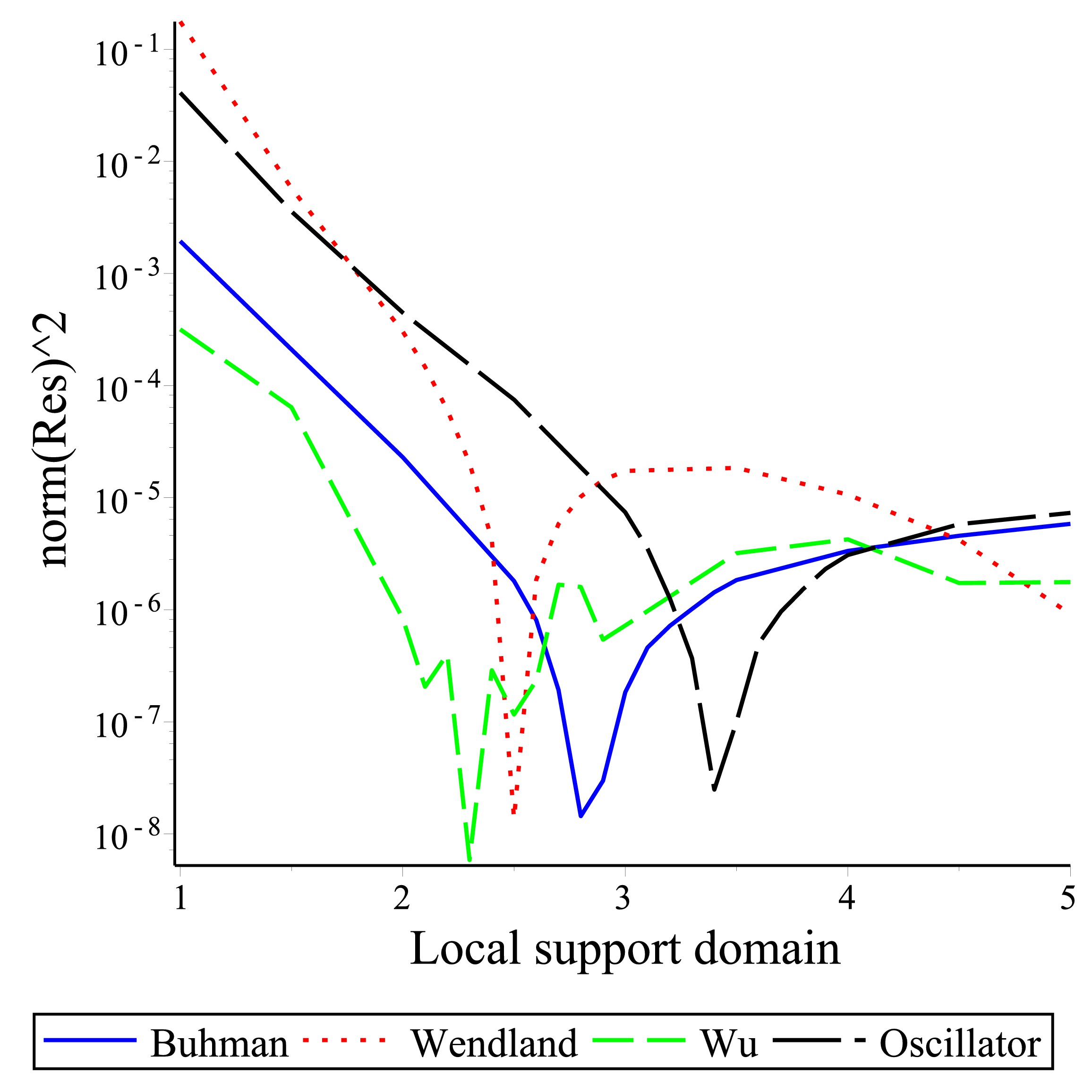
Figure 1: The graph of residual error versus local support domain when $N=30$, $\alpha=0.5$ and $xi=1.5$

3 Results and discussion

In this section, we compare the applied result of CSRBF with RBF methods [14] and yLWCM [17] .
In the physical observation of the unsteady gas problem, $y^{\prime}(0)$ has an important issue [1].Table 5 and 6. presents a comparison between the values of $y^{\prime}(0)$ and $y(x)$ for $\alpha=0.5$ and obtained by the CSRBF and, RBFs and yLWCM.

Table 5: Comparison of $y(x)$ for $\alpha=0.5$ with $\varrho=1.5$, $N=30$.

x	$Wendland_{3,5}$ $r_{\omega}=2.5$	$Wu_{3,3}$ $r_{\omega}=2.3$	$Oscillator_{3}$ $r_{\omega}=3.4$	$Buhman_{4}$ $r_{\omega}=2.8$	RBF.G	RBF.T	yLWCM
0.1	0.88136427	0.88136428	0.88136409	0.88136468	0.88139802	0.88137298	0.88147552
0.2	0.76582809	0.76582823	0.76582774	0.76582852	0.76588029	0.76579834	0.76661101
0.3	0.65599963	0.65999935	0.65599915	0.65600036	0.65606928	0.65590792	0.65727018
0.4	0.55389758	0.55389797	0.55389693	0.55389814	0.55399431	0.55375746	0.55567752
0.5	0.46094112	0.46094164	0.46094037	0.46094191	0.46107202	0.46078383	0.46325882
0.6	0.37797968	0.37798027	0.37797895	0.37798037	0.37814380	0.37783286	0.38078076
0.7	0.30535020	0.30535087	0.30534921	0.30535091	0.30554174	0.30522806	0.30853930
0.8	0.24295205	0.24295279	0.24295099	0.24295286	0.24316554	0.24285666	0.24644872
0.9	0.19033171	0.19033246	0.19033052	0.19033235	0.19056419	0.19025895	0.19409149
1.0	0.14677064	0.14677143	0.14677694	0.14677139	0.14702048	0.14671538	0.15877555
1.2	0.08313306	0.08313387	0.08313169	0.08313370	0.08341060	0.08310227	–
1.4	0.04404326	0.04404412	0.04404186	0.04404399	0.04433767	0.04402800	–
1.8	0.01002990	0.01003085	0.01002839	0.01003049	0.01034206	0.01002778	–
2.2	0.00170828	0.00170909	0.00170673	0.00170889	0.00202559	0.00170941	–
2.6	0.00021351	0.00021440	0.00021195	0.00021413	0.00053177	0.00021524	–
3.0	0.00001696	0.00001786	0.00001540	0.00001758	0.00033532	0.00001878	–
$\|Res\|^{2}$	1.3702e-08	5.8431e-9	2.4820e-08	1.4394e-08	8.52e-07	–	–

Table 6: Comparison of initial slope $y^{\prime}(0)$ for $\alpha=0.5$ with $\varrho=1.5$, $N=30$.

x	$Wendland_{3,5}$ $r_{\omega}=2.5$	$Wu_{3,3}$ $r_{\omega}=2.3$	$Oscillator_{3}$ $r_{\omega}=3.4$	$Buhman_{4}$ $r_{\omega}=2.8$	RBF.G	RBF.T	yLWCM
y’(0)	-1.191796	-1.191806	-1.191800	-1.191768	-1.191498	-1.191243	-1.199258

In addition, the value of $y^{\prime}(0)$ obtained by CSRBF methods for $n=20,30$ and various values of $\alpha$ are reported in Table 7.

Table 7: CSRBFs solutions of initial slope $y^{\prime}(0)$ with $N=20,30$

$\alpha$	$Wendland_{3,5}$		$Wu_{3,3}$		$Oscillator_{3}$		$Buhman_{4}$
	N=20	N=30	N=20	N=30	N=20	N=30	N=20	N=30
0.25	-1.15838196	-1.15658845	-1.15868018	-1.15652004	-1.16347841	-1.15658199	-1.15914956	-1.15651901
0.50	-1.19674806	-1.19179615	-1.19388602	-1.19180634	-1.19468231	-1.19180040	-1.19476755	-1.19176821
0.75	-1.23833094	-1.23998794	-1.23307537	-1.24033353	-1.23372756	-1.23980995	-1.23493307	-1.23984689

The stability of the CSRBF scheme depends on the local support domain $r_{\omega}$. An important unsolved problem is to find a approach to determine the optimal size of $r_{\omega}$. Also, The condition number grows with $N$ and $\varrho$ for fixed values of local support domain. Figure 2. and 3. shows the condition number of matrix $A$ versus local support domain $r_{\omega}$ and $\xi$.

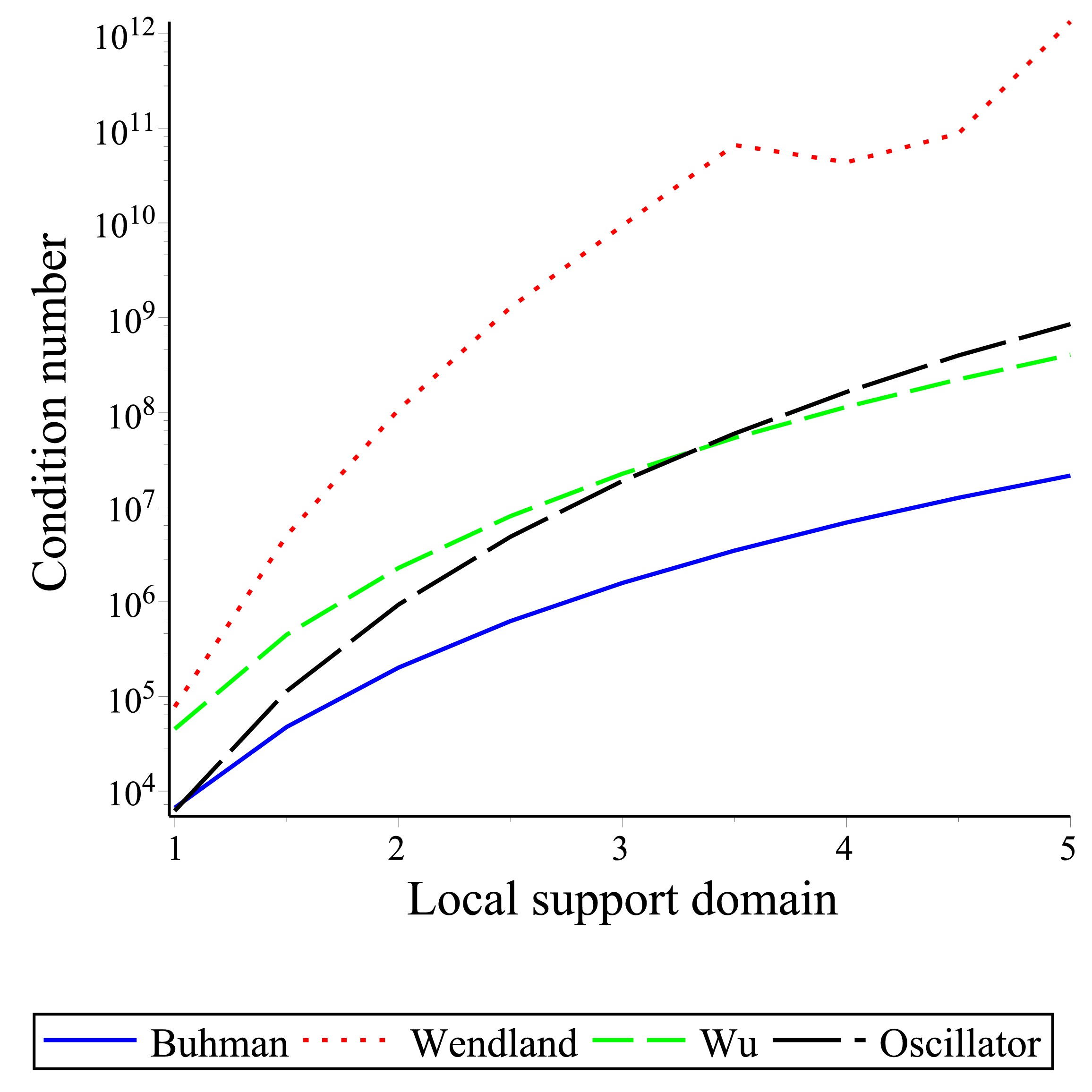
Figure 2: The graph of condition number versus local support domain when $N=30$, $\alpha=0.5$ and $\varrho=1.5$

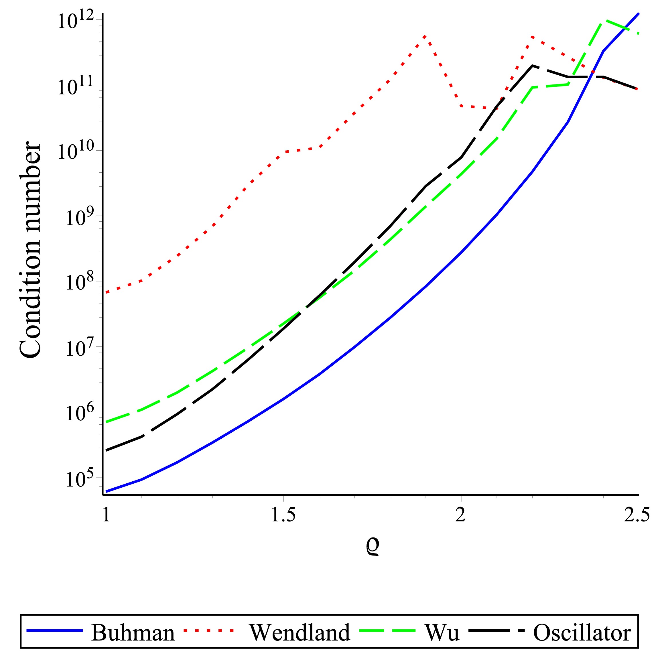
Figure 3: The graph of condition number versus $\xi$ parameter when $N=30$, $\alpha=0.5$ and $r_{\omega}=3$

Figure 2. shows that by decreasing the $r_{\omega}$, an increase is seen in the condition number of matrix $A$ and the method become more unstable. In general, the smaller the value of $r_{\omega}$, the higher percentage of zero entries in matrix $A$, so condition number matrix $A$ is a little and with increases the $r_{\omega}$, decrease percentage of zero entries in matrix $A$ and matrix $A$ will be unstable. A percentage of Zeros and condition number of CSRBFs in Matrix $A_{30\times 30}$ based on different values of local support domain $r_{\omega}$ illustrated in Table 8.

Table 8: A percentage of Zero and condition number in Matrix $A_{30\times 30}$.

$r_{\omega}$	$Zero$	$Wendland_{3,5}$	$Wu_{3,3}$	$Buhman_{4}$	$Oscillator_{3}$
1.0	64.44%	7.789055e04	4.532194e04	6.667960e03	6.196000e03
1.5	50.45%	5.005580e06	4.490489e05	4.762594e04	1.137094e05
2.0	38.55%	1.070687e08	2.277201e06	2.017929e05	9.349735e05
2.5	28.00%	1.284523e09	8.029373e06	6.255295e05	4.865744e06
3.0	19.33%	5.416534e09	2.248322e07	1.581147e06	1.886481e07
3.5	12.00%	6.652775e10	5.373891e07	3.469944e06	5.974023e07
4.0	06.33%	4.377016e10	1.142168e08	6.860756e06	1.642163e08
4.5	02.11%	8.799029e10	2.230297e08	1.252852e07	3.990271e08
5.0	00.00%	1.338415e12	4.055797e08	2.148696e07	8.539759e08

To find the critical values of $r_{\omega}$ , we use the residual error which can see in Figure 1. Figure 4. displays the $y(x)$ for $\alpha=0.5$ in Unsteady gas equation.

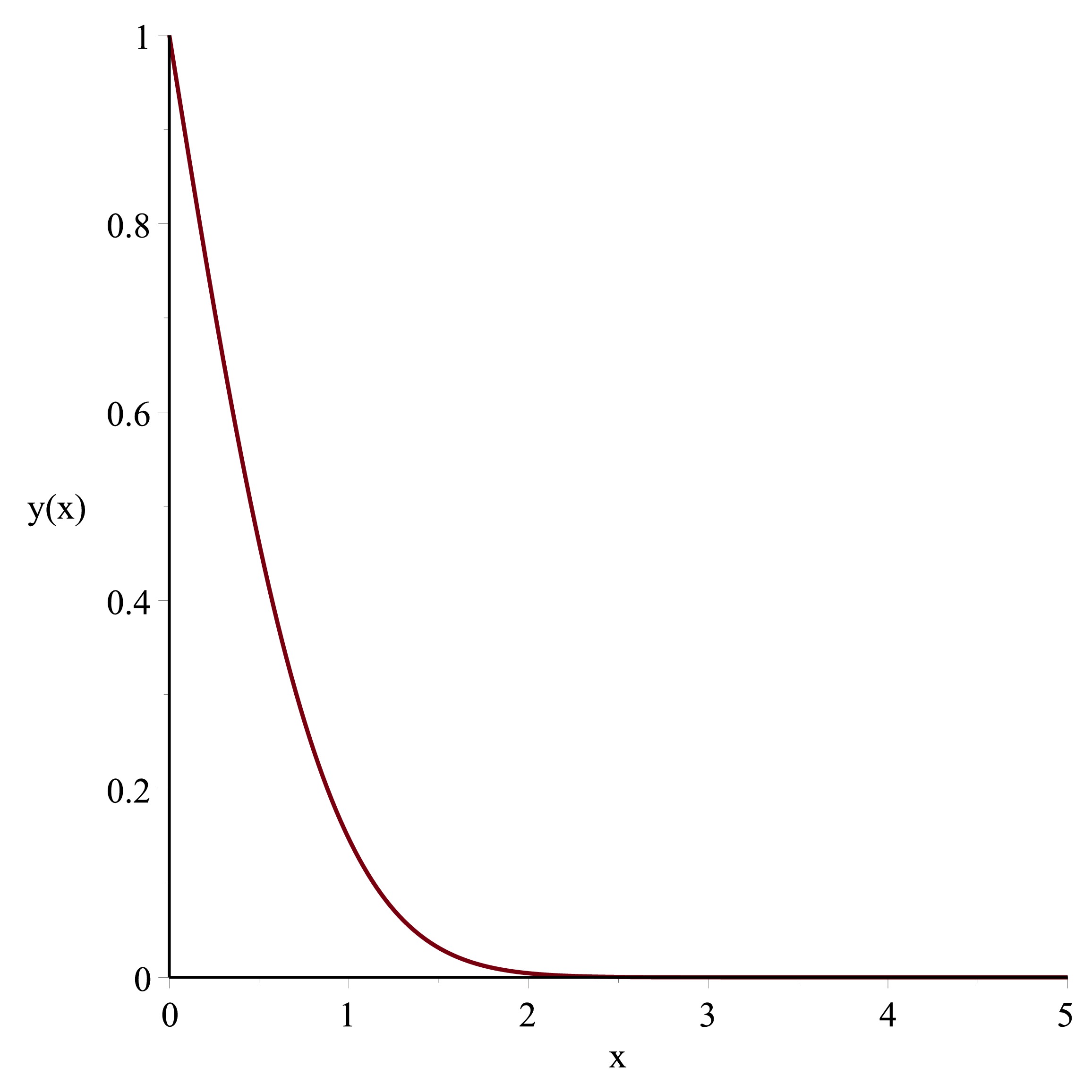
Figure 4: solution of $y(x)$ when $N=30$.

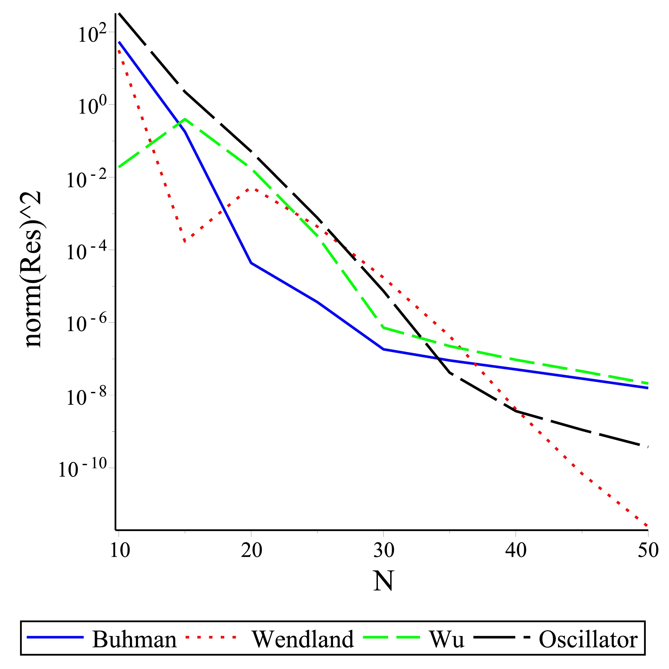
Figure 5: The graph of residual error versus $N$ when $r_{\omega}=3$, $\alpha=0.5$ and $xi=1.5$

in Figure 5. displays the convergence rates of the CSRBFs method for Eq. (8) for some value of $N$ for $\alpha=0.5$. These figures illustrate the convergence rate of the method.

4 Conclusion

The fundamental goal of this paper was the construct an approximation to the solution of unsteady gas equation. a set of CSRBFs with these properties were proposed for providing an effective but simple way to improve the convergence rate. A comparison was made among the solutions of [14, 17] and this work. the absolute error $\|Res\|^{2}$ were obtained. This paper has provided an acceptable method for Unsteady Gas equation. It was also confirmed by logarithmic figures of residual function that this method has an exponential convergence rate. Additionally, high convergence rate and good accuracy are obtained by the proposed method using relatively low numbers of collocate points.

References

- [1] R. E. Kidder, Unsteady flow of gas through a semi-infinite porous medium, J. Appl. Mech. 24 (1957) 329–332.
- [2] R. P. Agrawal, D. O’Regan, Infinite interval problems modelling the flow of a gas through a semi-infinite porous medium, Studies in Applied Mathematics , 108 (2002) 245–257.
- [3] R. C. Roberts, Unsteady flow of gas through a semi-infinite porous medium, Proceeding of the First US National Congress of Applied Mechanics , Ann Arbor, MI (1952) 773–776.
- [4] A. M. Wazwaz, The modified decomposition method applied to unsteady flow of gas through a porous medium, Appl. Math. Comput. 118 (2001) 123–132.
- Shokri and Dehghan [2010] A. Shokri, M. Dehghan, 2010. A not-a-knot meshless method using radial basis functions and predictor–corrector scheme to the numerical solution of improved boussinesq equation. Comput. Phys. Commun. 181, 1990–2000.
- Rashidi et al. [2014] K. Rashidi,H. Adibi,J. A. Rad, K. Parand, 2014. Application of meshfree methods for solving the inverse one-dimensional stefan problem,. Eng. Anal. Bound. Elem. 40, 1–21.
- [7] K. Parand, A. Taghavi, H. Fani, Lagrangian method for solving unsteady gas equation, Int. j. Comput. Meth. Sci. 3 (2009) 40–44.
- [8] K. Parand, M. Shahini, A. Taghavi, Generalized laguerre polynomials and rational chebyshev collocation method for solving unsteady gas equation, Int. j. Comput. Meth. Sci. 4 (2009) 1005–1011.
- [9] K. Parand, M. Nikarya, Solving the unsteady isothermal gas through a micro-nano porous medium via bessel function collocation method, j. Comput. Theor. Nano. 11 (2014) 1–6.
- Parand and Rad [2013] K. Parand, J. A. Rad, 2013. Kansa method for the solution of a parabolic equation with an unknown spacewise-dependent coefficient subject to an extra measurement. Comp. Phys. Commun. 184, 582–595.
- [11] J. A. Rad, K. Parand, Analytical solution of gas flow through a micro-nano porous media by homotopy perturbation method, World Academy of science Engineering and technology 4 (2009) 1188–1192.
- Rad et al. [2012] J. A. Rad, S. Kazem.,K. Parand, 2012. A numerical solution of the nonlinear controlled duffing oscillator by radial basis function. Comput. Math. Appl. 64, 2049–2065.
- Rad et al. [2014] J. A. Rad,S. Kazem,M. Shaban, K. Parand,A. Yildirim, 2014. Numerical solution of fractional differential equations with a tau method based on legendre and bernstein polynomials. Math. Meth. Appl. Sci. 37, 329–342.
- [14] S. Kazem, J. A. Rad, K. Parand, M. Shaban, H. Saberi, The numerical study on the unsteady flow of gas in a semi-infinite porous medium using an rbf collocation method, Int. J. Computer Math. 89 (2012) 2240–2258.
- [15] M. A. Noor, S. T. Mohyud-Din, Variational iteration method for unsteady flow of gas through a porous medium using he’s polynomials and padé approximants, Comput. Math. Appl. 58 (2009) 2182–2189.
- [16] Y. Khan, N. Faraz, A. Yildirim, Series solution for unsteady gas equation via mldm-padé technique, World Applied Sciences Journal 9 9 (2010) 1818–4952.
- [17] S. Upadhyay, K. N. Rai, Collocation method applied to unsteady flow of gas through a porous medium, Comput. Math. Appl. Res. 3 (2014) 251–259.
- [18] H. Roohani-Ghehsareh, S. H. Bateni, A. Zaghian, A meshfree method based on the radial basis functions for solution of two-dimensional fractional evolution equation, Eng. Anal. Bound. Elem. 61 (2015) 52–60.
- [19] N. S. O’Brien, K. Djidjili, S. J. Cox, Solving an eigenvalue problem on a periodic domain using a radial basis function finite difference schem, Eng. Anal. Bound. Elem. 37 (2013) 1594–1601.
- [20] C. A. Bustamante, H. Power, Y. H. Sua, W. F. Florez, A global meshless collocation particular solution method ( integrated radial basis function ) for two-dimensional stokes flow problems, Appl. Math. Model. 37 (2013) 4538–4547.
- [21] S. ul Islam, B. Sarler, R. Vertnik, G. Kosec, Radial basis function collocation method for the numerical solution of the two-dimensional transient nonlinear coupled burgers’ equations, Appl. Math. Model. 36 (2012) 1148–1160.
- [22] Q. Shen, A meshless scaling iterative algorithm based on compactly supported radial basis functions for the numerical solution of lane-emden-fowler equation, Numer. Methods Partial Differential Eq. 28 (2012) 554–572.
- [23] S. M. Wong, Y. C. Hon, M. A. Golberg, Compactly supported radial basis function for shallow water equations, Appl. Math. Comput. 127 (2002) 79–101.
- [24] H. Wendland, Piecewise polynomial , positive definite and compactly supported radial functions of minimal degree, Adv. Comput. Math. 4 (1995) 389–396.
- [25] H. Wendland, Scattered Data Approximation, Cambridge University Press, New York, 2005.
- [26] G. E. Fasshauer, Meshfree Approximation Methods With Matlab, World Scientific Publishing Co. Pte. Ltd., 2007.
- [27] G. E. Fasshauer, On smoothing for multilevel approximation with radial basis functions, Vanderbilt University Press,, 1999.
- [28] Z. Wu, Compactly supported positive definite radial functions, Adv. in Comput. Math. 4 (1995) 283–292.
- [29] T. Gneiting, Compactly supported correlation functions, j. Multivariate Analysis 83 (2002) 493–508.
- [30] M. D. Buhman, A new class of radial basis functions with compact support, Math. Comput. 70 (233) (2000) 307–318.
- Noye and Dehghan [1999] B. J. Noye, M. Dehghan, 1999. New explicit finite difference schemes for two-dimensional diffusion subject to specification of mass. Numer. Meth. Par. Diff. Eq. 15, 521–534.
- Dehghan and Shokri [2008] M. Dehghan, A. Shokri, 2008. A numerical method for solution of the two-dimensional sine-gordon equation using the radial basis functions. Math. Comput. Simul. 79, 700–715.
- Dehghan and Shokri [2009a] M. Dehghan,A. Shokri, 2009a. A meshless method for numerical solution of the one-dimensional wave equation with an integral condition using radial basis functions. Numer. Algorithms 52, 461–477.
- Dehghan and Shokri [2009b] M. Dehghan,A. Shokri, 2009b. Numerical solution of the nonlinear klein–gordon equation using radial basis functions. J. Comput. Appl. Math. 230, 400–410.
- Bu et al. [2015] W. Bu,Y. Ting,Y. Wu ,J. Yang, 2015. Finite difference/finite element method for two-dimensional space and time fractional bloch–torrey equations. J. Comput. Phys. 293, 264–279.
- Choi and Kweon [2016] H. J. Choi, J. R. Kweon, 2016. A finite element method for singular solutions of the navier–stokes equations on a non-convex polygon. J. Comput. Appl. Math. 292, 342–362.