Imperial College London
Department of Computing

 
Implementing a teleo-reactive programming system
 

Author:

Robert Webb

Supervisor:
Dr Anthony Field

Submitted in partial fulfillment of the requirements for the MSc degree in Advanced Computing of Imperial College London

Abstract

This thesis explores the teleo-reactive programming paradigm for controlling autonomous agents, such as robots. Teleo-reactive programming provides a robust, opportunistic method for goal-directed programming that continuously reacts to the sensed environment. In particular, the TR and TeleoR systems are investigated. They influence the design of a teleo-reactive system programming in Python, for controlling autonomous agents via the Pedro communications architecture. To demonstrate the system, it is used as a controller in a simple game.

*Acknowledgements

I would like to express my gratitude to Dr Anthony Field for his support and guidance throughout my project.

I would also like to thank Dr Keith Clark and Dr Peter Robinson for their support with the Qulog software and discussion in person and via email.

Finally, I thank my family, my friends and all my professors at Imperial College.

Chapter 0 Introduction

Teleo-reactive programming is a programming paradigm for autonomous agents (such as robots) that offers a way to deal with the unpredictable nature of the real world, as well as the challenge of connecting continuously-sensed inputs (percepts, sensed data) to outputs (actions). It incorporates ideas from control theory such as continuous feedback but it also incorporates features from computer science such as procedures and variable instantiation[Nilsson, 1994].

1 Objectives

One of the reasons why robotics is so challenging is that the real world is unpredictable. If a robot sets out to achieve some action, unexpected things might happen that “set back” the robot’s progress or cause the robot to fortuitously skip a few steps in its algorithm. Another challenge is that the world changes continuously, while computers and computer programs operate in terms of discrete time-steps. Teleo-reactive programming both of these problems by allowing robust (able to recover from setbacks) and opportunistic (able to take advantages of fortuitous changes in the environment) computer programs to be developed, that also continuously react to their sensed environment.

This report aims to describe in detail the seminal teleo-reactive system TR[Nilsson, 1994, 2001] and the later system TeleoR[Clark and Robinson, 2014a, b], which adds additional features to the original system. It also describes the Pedro communications protocol, which is used by TeleoR for inter-agent communication.

This report also describes a teleo-reactive system developed for this thesis project, which consists of an interpreter of a TR-like language which can communicate a simulation via Pedro, implemented in Python. The syntax and semantics (how the language is evaluated) will be explained in detail.

The teleo-reactive system will be demonstrated controlling a simple demonstration program. Sample teleo-reactive programs and explanations of their meaning are given. The report will also discuss whether teleo-reactive solves the problem of robot control well, what alternatives to TR and TeleoR exist, the alternatives to teleo-reactive programming and the miscellaneous practical considerations made when developing this project.

2 Overview

The structure of the report is as follows:
Chapter 1 provides background knowledge, describing Nilsson’s TR system and Clark & Robinson’s TeleoR system.
Chapter 2 describes the language of the system that was developed at a high level, covering the syntax.
Chapter 3 describes in more detail how the system works, the algorithms involved, the type system and what programs are (in)valid.
Chapter 4 presents a demonstration of the teleo-reactive system, gives an evaluation of the success of the system, the alternative teleo-reactive systems (other than TR and TeleoR) that have been developed, alternatives to teleo-reactive programming and practical decisions made during the project.
Chapter 5 sums up the project and suggests future related areas of research.

Chapter 1 Background

1 Teleo-reactive programming

Teleo-reactive programming involves creating programs whose actions are all directed towards achieving goals, in continuous response to the state of the environment. It offers a way to specify robust, opportunistic and goal-directed robot behaviour [Clark and Robinson, 2014a]. This means that it recovers from setbacks and will skip unnecessary actions if it can[Clark and Robinson, 2014b].

This section will explain teleo-reactive programming, by describing Nilsson’s TR language[Nilsson, 1994, 2001]. It will then describe TeleoR, a language by Clark and Robinson that extends the semantics of TR while adding performance optimisations and facilities for multi-agent programming. The two languages are intended as mid-level languages, they act as an interface between the senses and the actions performed by the agent[Clark and Robinson, 2014b].

1 Continuous evaluation

Designing autonomous agents is difficult because they must operate in a constantly changing environment which can be sensed only imperfectly and only affected with uncertain results. However, autonomous agents have been developed in other domains that do function effectively in the real world for long periods of time. For example, governors that control the speed of steam engines, thermostats and complex guidance systems. One thing that these systems have in common is that they continuously respond to their environment[Nilsson, 1992].

Nilsson proposes teleo-reactive programming as a paradigm that allows programs to be written that continuously respond to their inputs in a similar way that the output of an electronic circuit continuously responds to its input signals, but retains useful concepts from computer science such as hierarchical organisation of programs, parameters, routines and recursion[Nilsson, 1992]. He refers to computer programs that continuously respond to their inputs as having “circuit semantics”. Nilsson also intended for teleo-reactive programs to be responsive to the agent’s stored model of the environment, as well as directly sensed data[Nilsson, 1994].

2 TR

The TR language is Nilsson’s implementation of teleo-reactive programming[Nilsson, 2001]. This chapter will describe the design and features of the TR language, then explore the later TeleoR language which adds additional features to TR.

1 Triple-tower architecture

At the most abstract level, Nilsson splits the problem of decision making in autonomous agents into three tasks, which are performed by the triple-tower architecture[Nilsson, 2001]. The three parts of the system that perform these three tasks are called the “towers” of the architecture, because they work at multiple levels of abstraction, that incrementally build on lower layers. The three towers are:

• the perception tower - deducing further truths about the world (rules);

• the model tower - maintaining the agent’s knowledge about the world (predicates and truth maintenance system);

• the action tower - deciding what course of action to take (action routines);

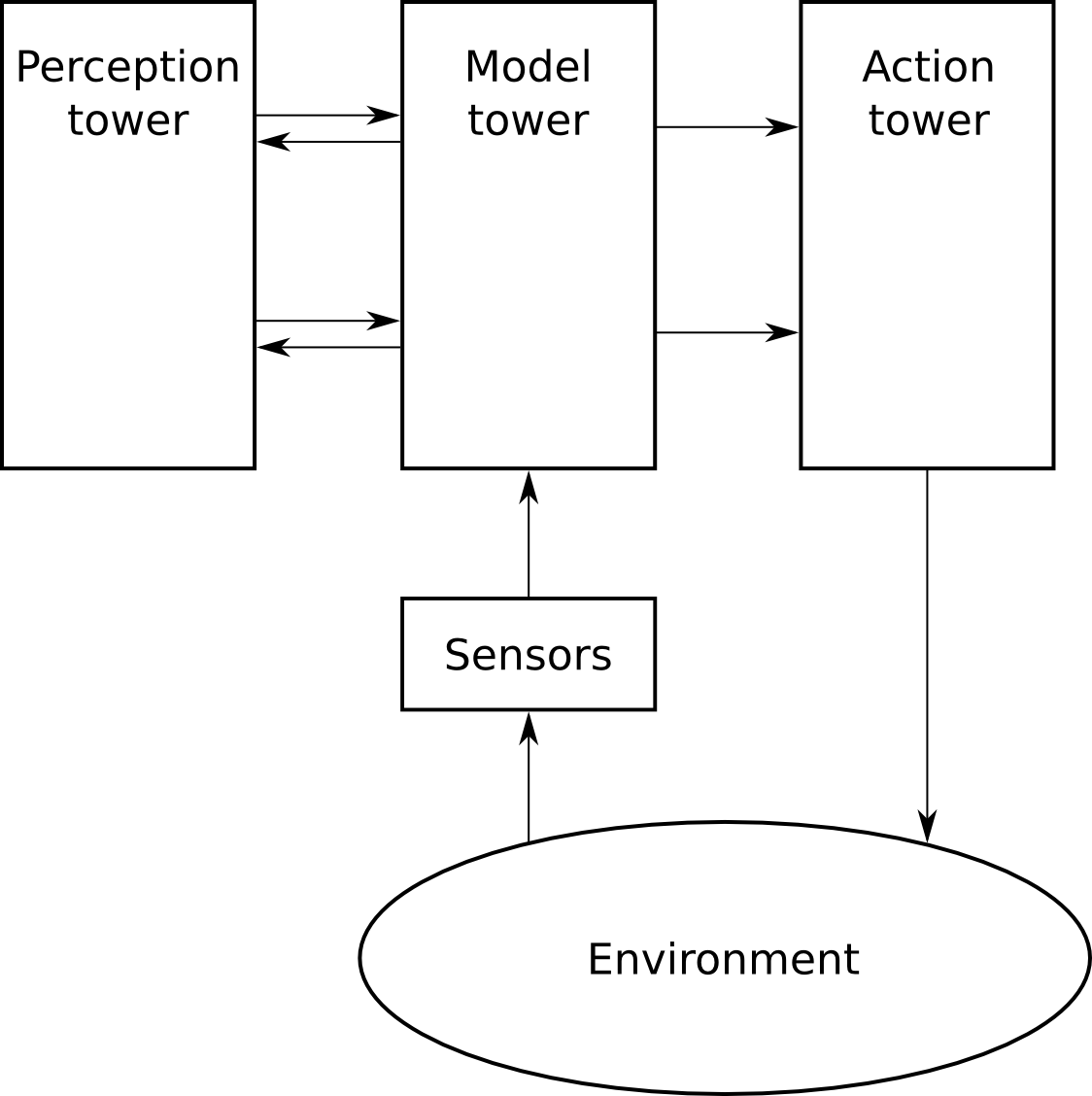
Figure 1: Diagram of the triple-tower architecture

Perception tower

The first tower is the perception tower. It consists of logical rules that are used to deduce new facts from existing knowledge. These can be expressed using a logic programming language. Each rule can be defined in terms of other rules, hence the “tower” nature of the perception tower. The perception tower creates higher-abstraction percepts from lower-abstraction ones[Nilsson, 2001].

For example, consider a scenario with a percept on(X,Y), objects block(X) (uniquely numbered, for $X\in\mathbb{N}$), the object table and the object nothing. on(X,Y) means that the object X is on top of the object Y. From this basic percept, a new predicate sorted_stack(X) can be defined which states that the block X is at the top of a stack of blocks, where the blocks are sorted with block(1) at the top and the highest numbered block at the bottom. This could be defined as follows:

sorted_stack(table).

sorted_stack(block(1)) :- on(empty, block(1)),
                          on(block(1), X),
                          sorted_stack(X).

sorted_stack(block(N)) :- on(block(N),
                          block(M)),
                          N >= M,
                          sorted_stack(block(M)).

This new predicate sorted_stack(X) can now be queried by another part of the program. This example uses Prolog expressions.

Model tower

The model tower consists of a truth-maintenance system that invokes the rules in the perception tower on the percepts sensed by the agent. The goal of the TMS is to keep the agent’s knowledge continuously faithful to changes in the environment[Nilsson, 2001].

Action tower

The action tower specifies what actions the robot should perform, based on the knowledge maintained by the model tower. It should be possible to define actions in terms of other (sub-)actions, so that complex behaviours can be defined in terms of simpler ones. For example, picking up a box involves moving an arm, opening and closing a gripper, etc.

The TR language was designed by Nilsson to perform the role of the action tower. Given facts about the world (percepts) and the robot’s knowledge (stored beliefs and predicates inferred from the beliesf and percepts), the robot can autonomously perform actions based on a series of rules[Nilsson, 2001]. The next few sections will explain what the TR language is and how it can be used.

2 TR sequences

The distinctive feature of teleo-reactive programming is the TR sequence, which is an ordered sequence of rules of the form “if some conditions are satisfied, then perform these actions”[Nilsson, 1994]. The conditions, or guards are defined in terms of percepts and beliefs. Percepts are information that has been sensed by the agent and beliefs are facts remembered by the agent. An action can be either be a tuple of primitive actions to be performed concurrently (e.g. move forward, turn left, look up) or a call to initiate another TR sequence[Clark and Robinson, 2014b].

The actions currently being performed by the agent are defined as the actions associated with the first satisfied condition in the TR sequence. If no condition of any of the rules can be satisfied, an error occurs, so the last rule is sometimes written so that it always fires (being a ‘none of the above’ condition)[Clark and Robinson, 2014b].

K_1 ~> A_1
K_2 ~> A_2
...
K_n ~> A_n

In order for a TR sequence to achieve a goal, the rules are written in a way that the topmost rule describes the goal state and every other rule brings the agent closer to satisfying the guards of the rules above them. A TR sequence with this feature is referred to as having the regression property. If a TR sequence has the regression property and a guard can always be satisfied (e.g. if the bottommost rule always applies), then it is a universal program[Clark and Robinson, 2014b].

Example

To give a simple example of a TR sequence, imagine a 2D world where there is a robot and a light. The goal of this procedure is for the robot to turn to face the light.

• The first rule defines the condition that the procedure is supposed to achieve - the robot is facing the light, in which case, do nothing.

• The second rule says that if the robot sees the light to the left of it, then turn left.

• The third rule says that if the robot sees the light to the right of it, then turn right.

• The fourth rule is fired if the robot does not see anything - it continually turns left until something comes into view that triggers the upper rules.

is_facing(light) ~> ()
see(light, left) ~> turn(left)
see(light, right) ~> turn(right)
() ~> turn(left)

3 TR procedures

Goals can be split into sub-goals, sub-sub-goals and so on, so to reflect this teleo-reactive programs can also be written in a hierarchical and structured way, using TR procedures. A TR procedure is a TR sequence that can be called by another TR sequence. Just like a procedure in a structured imperative language, it has a name and takes a tuple of parameters as input. TR procedures can be written that achieve sub-goals, that are then called by procedures to achieve higher goals [Clark and Robinson, 2014a]. For example, a program that tells an agent to pick up a box with a robotic arm could be made up of:

• a procedure that tells the agent to face the box

• a procedure that tells the agent to move forwards to the box

• a procedure that tells the agent to pick up the box that is in front of it

The syntax of a TR procedure is as follows:

procedure_name(param_1, param_2, ... , param_k){
  K_1 ~> A_1
  K_2 ~> A_2
  ...
  K_n ~> A_n
}

procedure_name is the name of the procedure, param_1, ... , param_k are names of the parameters passed to the procedure.

Guards in TR procedures can be partially instantiated, which means that some (or none) of the variables in the guard are from the parameters of the procedure, some are constant terms and some become instantiated when the rule is satisfied[Clark and Robinson, 2014b]. While not all variables on the left hand side of the rule have to be instantiated, all variables on the right hand side must be instantiated, otherwise an error is thrown. The ability to write rules in this way means that more general rules can be written, making the program code shorter and more readable.

Example

The procedure from the previous example could be rewritten as a TR procedure:

face_thing(Thing){
  is_facing(Thing) ~> ()
  see(Thing, Dir) ~> turn(Dir)
  () ~> turn(left)
}

Calling this procedure as face_thing(light) causes the variable Thing to be instantiated to light. Rewriting the original sequence as a procedure means that the robot can be told to face many different things, using the same code. The second and third lines of the original sequence have also been combined into a single rule. If the robot sees the light to the left hand side, then Dir is instantiated as left and the action turn(left) is performed. Likewise, if the robot sees the light to the right hand side, then Dir is instantiated as right and the action turn(right) is performed.

TR algorithm

Figure 2: Flowchart depicting the TR algorithm

The flowchart on the previous page (Figure 2) describes an informal algorithm[Clark and Robinson, 2014a] for executing TR programs. It describes the operation of a TR program that has been called with the call $TaskCall$. $FrdRules$ is the set of indexed active procedure calls. Each element of $FrdRules$ is a tuple of the form $(Dp,Call,R,\Theta)$ where $Dp-1$ is the number of intermediary procedure calls between $Call$ and $TaskCall$, $R$ is the number of the partially instantiated rules of the procedure for $Call$ that was last fired and $\Theta$ is the set of generated bindings for all the variables of the action of that rule. $Dp$ is the index of the tuple. $Acts$ is the last tuple of determined actions for $TaskCall$, initialised to $()$.

Step 1 initialises the state of the algorithm, which consists of $LActs$, $FrdRules$, $Index$ and $Call$.

Step 2 is the first step of the execution loop of the program, it checks that the maximum call depth has not been exceeded. The maximum depth is defined by the programmer with the parameter $MaxDp$. Step 3 finds the first rule in the current call. If no rule is fired, the algorithm goes to step 9 and fails. If a rule is found, the algorithm goes to step 3b. If the rule’s action (with variables instantiated) is a procedure call, then call the procedure and go back to step 2. If it is a tuple of primitive actions, go to step 6 and compute the controls and execute them, then go to step 7.

At step 7, wait for a BeliefStore update (i.e. a modification to the beliefs and percepts), then set $Index$ to $1$. Step 8 and 8b consist of a loop that checks every previously fired rule from the last call to see if it must continue to fire. This is done by keeping track of which predicates must be true or false to satisfy the guard conditions for each rule firing. If every previously fired rule has been found to continue, go back to step 7. Otherwise, go to step 11.

At step 11, re-evaluate the guards in the same way as in step 3 to find the rule that must now fire. If the rule and variable substitution are the same, go to step 10. If either of them are different, update $FrdRules$ so that the old rule at the current level in the call stack is replaced by the new rule, then go to step 3b. If no rule can be found, go to step 9 (failure)[Clark and Robinson, 2014b].

4 Continuation of firings

From the rule definitions, it is possible to know which predicates would have been queried to find the first fireable rule. With this information, it is possible to determine the conditions (i.e. which predicates must be inferable or not inferable) under which it would continue to fire.

There are only two ways in which a currently firing rule can be interrupted:

• The guard of a rule above the previously fired rule becomes inferable;

• The conditions for the previously fired rule become inferable for a different instantiation of variables.

Therefore, unless one of these two conditions holds, there is no need to re-evaluate the guards of the TR procedure. This can be expressed in terms of the “local dependent predicates” for a given rule, inside a TR procedure. This is a list of predicates, that if they were to become inferable / not inferable, would cause a given rule to no longer continue to fire. This is defined as a list of functors (names of predicates), prefixed with a symbol. If a predicate prefixed with a ++ is added to the belief store (either as a fact or rule), then the rule might stop firing. If a predicate prefixed with -- is removed from the belief store, then the rule might stop firing. For example, consider the below procedure:

proc1(){
a & b ~> m1
d & e ~> m2
f & g ~> m3
true ~> m4
}

The “local dependent predicates” for the first rule are [--a, --b].
For the second rule they are [--d, --e, ++a, ++b].
For the third rule they are [--f, --g, ++a, ++b, ++d, ++e].
For the last rule they are [++a, ++b, ++d, ++e, ++f, ++g].

To check if a rule must continue firing, the union of all of the local dependent predicates of all of the rule’s parent calls is calculated to produce the “dependent predicates” of the current state of the program[Clark and Robinson, 2014a].

To demonstrate this, consider the following program:

proc1(){
a & b ~> c
d & e ~> f
f ~> proc2()
true ~> g
}

proc2(){
k ~> l
m ~> n
true ~> q
}

Say the program was called by calling the proc1 procedure. If the second rule of proc2 is currently firing (as a result of the third rule of proc1 being fired), the “dependent predicates” can be determined by finding the union of the local dependent predicates for the third rule of proc1 and the second rule of proc2.
These are:
proc1, rule 3: [++a, ++b, ++d, ++e, --f].
proc2, rule 2: [++k, --m].

So the dependent predicates are [++a, ++b, ++d, ++e, --f] $\cup$ [++k, --m] $=$ [++a, ++b, ++d, ++e, --f, ++k, --m].

5 Evaluation of TR conditions

In Nilsson’s 2001 paper[Nilsson, 2001] introducing the “Triple Tower Architecture”, the inference rules in the Perception Tower were used to populate the Model Tower with derived knowledge but the way in which this is done is not elaborated on. However, there are papers have given formal semantics for TR, such as [Dongol et al., 2014] in a temporal logic and [Kowalski and Sadri, 2012] as abductive logic programming. Nilsson mentions that the “not” expression in TR means “negation-as-failure” so (given the fact that the rules in the “Perception Tower” resemble Horn clauses) it is reasonable to assume that TR uses SLDNF (Selective Linear Definite clause resolution with Negation by Failure)[Sergot, 2010].

3 TeleoR/Qulog

TeleoR is a language devised by Keith Clark and Peter Robinson as an extension of the original language TR[Clark and Robinson, 2014b]. The declarative logic/functional language used to express guard conditions, relations (predicates) and functions is called Qulog. The added features are as follows:

• procedures and the BeliefStore language (Qulog) are typed and allow for higher order programming;

• timed action sequences that can specify a sequence of actions to be executed cyclically;

• while/until rules which allow the programmer to provide additional conditions under which the rule can fire;

• wait/repeat actions can be given, which lets a discrete action be repeated if it has not resulted in the firing of another rule within some period of time. This is useful in cases where an action does not have the desired effect first time (e.g. if something in the robot mechanism jams);

• actions are provided that dynamically modify the BeliefStore, so that that agent can “remember” and “forget” facts;

• the ability to link BeliefStore updates and message send actions to any other agents with any rule action, allowing for inter-agent communication.

1 Two-tower architecture

The high-level design of TeleoR is different to that of TR in that it does not include a truth maintenance system. The three-tower architecture becomes a two-tower architecture, with two towers:

• the BeliefStore tower - this deduces truths about the world from the incoming percepts, essentially having the same functions as the perception tower in TR.

• the Action tower - this performs the same role as the action tower in TR, although the language used to determine the actions to perform is different, with some added features.

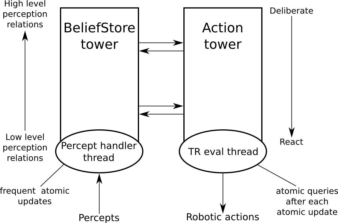
Figure 3: Diagram of the two-tower architecture

2 TeleoR Syntax

Now for the syntax of the TeleoR language. A procedure takes the following form. Like in the description of TR, procedure_name is the name of the procedure and param_1, ... param_k are the names of the parameters. Added to the procedure definition is a type declaration, where t_i is the type of parameter param_i.

procedure_name : (t_1, ..., t_k) ~>
procedure_name(param_1, ... , param_k){
  G_1 while WC_1 min WT_1 until UC_1 min UT_1 ~> R_1
  G_2 while WC_2 min WT_2 until UC_2 min UT_2 ~> R_2
  ...
  G_n while WC_n min WT_n until UC_n min UT_n ~> R_n
}

The first line is new to TeleoR, it is a type signature. It states which types of parameters can be passed to the procedure. The way in which types are checked and how this aids development will be discussed in another section. The left-hand side of each rule has also become more complex, these are the aforementioned “while/until” conditions. These are explained in the “Guard conditions” section. If a part of the guard contains vacuous constraints (i.e. constraints that do not alter the behaviour of the rule) then they can be omitted. The right-hand sides of the rules ($R_{1}$ to $R_{n}$ are also more complex than for TR. Not only can they contain a tuple of action primitives or a call to a procedure, they can contain expressions of the form:

A_1 for N_1; A_2 for N_2; ... ;A_m for N_m
A wait N_1 repeat N_2

where $A_{i}$ are either primitive actions to be executed in parallel (separated with commas) or single procedure calls. The semantics of the timed sequence actions and the wait/repeat actions will be explained later.

3 The BeliefStore in TeleoR

“BeliefStore” is a term used to describe whatever the source of percepts and beliefs in the teleo-reactive system is. In the case of TeleoR it is the language QuLog, which was also developed by Clark and Robinson. The language itself will be described in more detail later in this chapter[Clark and Robinson, 2014a] in Section 6, 7 and 8.

4 Extensions to TR rules

Guard conditions

In TeleoR, the language of guard conditions has been made more expressive. This has been done by the introduction of while and until conditions. These are of the form[Clark and Robinson, 2014b]:

G while WC min WT until UC min UT ~> A

This means that once the rule has begun to fire, it will continue to fire while (Equation 1) holds (the continuation condition).

$$\mathtt{inferable}(G)\lor((\mathtt{inferable}(WC)\lor\neg\mathtt{expired}(WT))\land(\neg\mathtt{inferable}(UC)\lor\neg\mathtt{expired}(UT)))$$ (1)

where $\mathtt{inferable}(X)$ means that the query $X$ is currently inferable and $\mathtt{expired}(T)$ means that more than $T$ seconds have elapsed since the rule started firing. If WC or UC are not given, they default to false. If WT or UT are not given, they default to 0. If X is 0, then $\mathtt{expired}(X)$ wil always be true. So, based on the original form, the following variations are possible:

G while WC min WT until UC

has the corresponding (simplified) continuation condition (Equation 2).

$$\mathtt{inferable}(G)\lor((\mathtt{inferable}(WC)\lor\neg\mathtt{expired}(WT))\land\neg\mathtt{inferable}(UC))$$ (2)

G while WC until UC min UT

has the corresponding (simplified) continuation condition (Equation 3).

$$\mathtt{inferable}(G)\lor(\mathtt{inferable}(WC)\land(\neg\mathtt{inferable}(UC)\lor\neg\mathtt{expired}(UT)))$$ (3)

G while WC min WT

has the corresponding (simplified) continuation condition (Equation 4).

$$\mathtt{inferable}(G)\lor(\mathtt{inferable}(WC)\lor\neg\mathtt{expired}(WT))$$ (4)

G while WC until UC

has the corresponding (simplified) continuation condition (Equation 5).

$$\mathtt{inferable}(G)\lor(\mathtt{inferable}(WC)\land\neg\mathtt{inferable}(UC))$$ (5)

G

has the corresponding (simplified) continuation condition (Equation 6).

$$\mathtt{inferable}(G)$$ (6)

The effect of while and until conditions is confined to the procedure-level. This means that if a rule in some procedure is fired but the procedure stops being called, the rule’s action will always stop firing, regardless of any while/until conditions that the rule may have[Clark and Robinson, 2015].

The behaviour of the while/until rules can be illustrated with diagrams showing example rule firings. Consider the rule G while WC min WT until UC min UT ~> A, where WT > UT. In the first case (Figure 4), the rule fires, then WC becomes inferable just after WT seconds, then the rule stops firing after WC stops being inferable. In the second case (Figure 5), the rule fires then UT becomes inferable, but it does not stop the rule from firing, then it stops being inferable. Then it becomes inferable again, but because this happens after UT seconds, it causes the rule to stop firing.

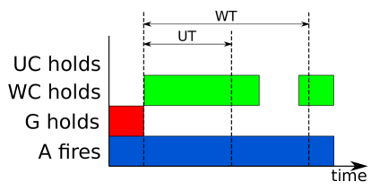
Figure 4: Example rule firing

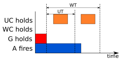
Figure 5: Example rule firing

Timed sequences of actions

A_1 for T_1; T_2 for T_2; ... ;A_m for T_m

The above action performs m actions in sequence. A_1 is performed for N_1 seconds and then A_2 will be performed for N_2 seconds and so on until A_m then the agent will start at A_1 again [Clark and Robinson, ]. A_i can be a tuple of primitive actions or a procedure call. If for T_m is missing, then the corresponding action will run indefinitely, until the rule stops firing.
For example, given a robot with a turn/1 durative action that takes a direction as input (direction ::= left | right) and a move_forward/0 durative action, a task could be defined that causes the robot to move in a zig-zag motion:

zigzag : () ~>
zigzag(){
true ~> move_forward, turn(left) for 0.2;
        move_forward, turn(right) for 0.2
}

In this example, the robot moves forward and turns left for 0.2 seconds, then moves forward and turns right for 0.2 seconds, then moves forward and turns left for 0.2 seconds and so on.

Timed sequence actions can also be used to tell the agent to do some things, then do one thing forever. For example, the task move_forward_then_turn_left could be defined as follows:

move_forward_then_turn_left : () ~>
move_forward_then_turn_left(){
true ~> move_forward for 1;
        turn(left)
}

This task tells the agent to move forward for 1 second, then turn left indefinitely.

wait … repeat actions

The wait … repeat construct allows an action to be tried, then retried a number of times at a given interval. This can be useful if the agent has to perform an action that may not succeed and may have to be retried. For example, if a door-opening grabs and turns a handle on a door, then it could be programmed to retry if the door does not open. It has the following syntax:

A wait T repeat R

The above code will perform the action A and after T seconds the action A will be tried again a maximum of R times unless another rule is chosen. If no rule is chosen after R repeats, an error is generated action_failure which appears as a percept which can be queried by the parent procedure [Clark and Robinson, 2014b, 2015].

For example, if an agent is programmed to open a door by pushing it (where push is a discrete action), it may not succeed on the first try (e.g. the door is jammed or is locked). So the wait/repeat construct can be used to retry the action a given number of times. In this example, if the do_things procedure is called then if agent sees a closed door then it will call open_the_door which (unless an open door is already observed) will cause the robot to push on the door, wait one second, then push on the door three more times at one second intervals. If no other rule is fired by that point, a special action_failure percept will be remembered, which will cause the first rule in do_things to fire. The robot can now deal with the fact that open_the_door had failed, e.g. by using a key (to unlock the door).

do_things(){
action_failure ~> use_key()
see(closed_door) ~> open_the_door()
true ~> ()
}

open_the_door(){
see(open_door) ~> ()
true ~> push wait 1 repeat 3
}

remember, forget actions

The TeleoR language provides primitive actions to add and remove beliefs dynamically from the BeliefStore, which can be used to give the agent some ‘memory’ or state. This is done with the remember and forget actions. The remember action adds a belief to the BeliefStore and the forget action removes a belief. These beliefs can be queried in the guards of the rules like the percepts[Clark and Robinson, 2014a]. The belief must have been declared as a belief (with a type) [Clark and Robinson, 2015].

5 Example TeleoR Programs

I will now give some example programs, that illustrate how TeleoR programs can be designed.

Teleo-reactive programming is ideal for expressing the behaviour of systems whose behaviour reacts continuously to the outside world. One such system is a thermostat. This is a machine that switches a heater on and off, in order to keep a room or other space at a certain temperature. In its simplest form, it consists of a thermometer that turns on a switch if the temperature is above (or below) a certain desired level. If the temperature is too low, the heating is turned on, if it is too high then the heating is turned off. This behaviour has been expressed in the following teleo-reactive program.

discrete turn_on_heating : (),
         turn_off_heating : ()

percept  is_too_cold : ()

thermostat_task : () ~>
thermostat_task(){
is_too_cold ~> turn_on_heating
true ~> turn_off_heating
}

This program has two actions turn_on_heating and turn_off_heating, and one percept is_too_cold which becomes inferable if the temperature of the room is too cold. In order to run the program, the thermostat_task procedure is called, with no arguments.

The next program generalises the above program, to take the desired temperature as an argument.

discrete turn_on_heating : (),
         turn_off_heating : ()

percept temperature : (num)


regulate_temperature : (num) ~>
regulate_temperature(Target){
temperature(Temperature) & Temperature < Target ~> turn_on_heating
true ~> turn_off_heating
}

The is_too_cold percept from the first example has been replaced with a temperature percept which, as stated in its type signature, has one term which is of type num (a number). If the percept temperature(T) is inferable, it means that the temperature is T degrees Celsius. The regulate_temperature task also takes a parameter, which is the temperature that the thermostat must maintain. So the temperature that the thermostat can be chosen by whatever calls the procedure. The first rule in the procedure states that if a certain temperature is sensed, if that temperature is lower than the desired temperature, then turn on the heating. The second rule covers all other cases (i.e. no temperature detected or the temperature was equal or greater than the desired temperature), in which case the heating is turned off. Now we have a general-purpose procedure for a thermostat that can maintain any temperature. This can then be re-used in another part of the program, as the following example will show:

discrete turn_on_heating : (),
         turn_off_heating : ()

percept temperature : (num),
        person_in_room : ()


thermostat_behaviour : () ~>
thermostat_behaviour(){
person_in_room ~> regulate_temperature(28)
true ~> regulate_temperature(18)
}

regulate_temperature : (num) ~>
regulate_temperature(Target){
temperature(Temperature) & Temperature < Target ~> turn_on_heating
true ~> turn_off_heating
}

This program introduces a new procedure thermostat_behaviour and a new percept person_in_room which is inferable if a person is detected in the room. The thermostat_behaviour procedure states that if a person is sensed in the room, maintain the temperature at 28 degrees, otherwise maintain it at 18 degrees. It shows how (like in other programming paradigms) procedures can be re-used to incrementally build up more complex behaviour. Another thing to note is that because of the type signatures given by the programmer, this program can be proven at compile time to never produce a run-time type error (unless provided with invalid percepts or arguments). The signature of regulate_temperature states that the argument must be a number, in both cases in thermostat_behaviour it is called with numbers (18 and 25). Given that, it is guaranteed that Target will not cause a type error when compared with Temperature (because Temperature is of type num, given the type signature of temperature).

6 Relation definitions

Relations can be defined in QuLog using two constructs: Unguarded Rules and Guarded Rules. The definition of the syntax of these rules is copied from the paper describing QuLog [Clark and Robinson, ].
Unguarded Rules have the following syntax:

Head
or
Head <= ComplexConj

where Head is a head predication of the form rel(Arg1, …, Argk) where k > 0.
A ComplexConj has the form Cond1 & ... Condn, $n\geq n$, with Condi being:

• a body predication RelExp(Exp1, ... , Expk), $k\geq 0$, where each Expi is an expression - a term that may contain function calls. RelExp is an expression returning a k-ary relation rel’ such that the values of the argument expressions will satsify the mode and type constraints of rel’ when it is called.

• a body predication prefixed with not, the QuLog negation-as-failure

• a body predication prefixed with once, indicating that only one successful evaluation should be found

• an expression value unification Exp1 = Exp2

• a non-deterministic pattern match Exp =? PtnTerm

• a meta-call call Call, of type !relcall

• a universally quantified implication (a forall) of the form: forall V1, ... , Vj (exists $EVarsSeq_{1}$ $SimpleConj_{1}$ => $EVarsSeq_{2}$ $SimpleConj_{2}$), $j\geq 1$
  The Vi variables are universally quantified over the implication. The sequence of variables of EVarsSeqi are existentially quantified over SimpleConj1 and SimpleConj2.

A SimpleConj is a ComplexConj that does not contain any forall.
Guarded Rules are of the following form:

Head :: Commit <= Body

Commit is a SimpleConj and Body is a ComplexConj.

The Commit is a test that, if passed, no other definitions will of the relation will be considered. So the above definition is similar to Head :- Commit, !, Body in Prolog, but Qulog does not have the cut (!) operator.

Every relation has a Relation Type Declaration, which states the type and mode of the terms of the relation. It is of the form:

rel: (m1t1, ... , mktk) <=

where rel is the name of the relation, ti is the ith type expression and each mi is one of the three prefix mode annotations !, ?, ??. If the type is omitted, then the type term is used (i.e. any type of term is accepted). The postfix ? is equivalent to ?? and the prefix ! can be dropped[Clark and Robinson, ].

7 Function definitions

Functions can be expressed in two ways:

fun(Arg0, ... , Argk) -> Exp
or
fun(Arg0, ... , Argk) :: SimpleConj -> Exp

Like in the rule definitions, the SimpleConj is the “commit test”. fun(Arg0, ... , Argk) is the head of the function definition. To evaluate a function call, the expressions Arg0, ... , Argk are first evaluated. Then, the first rule for fun with a head that matches the argument call and passes the commit test (if any) determines the call’s value. This is the value of the right hand side expression Exp, made ground by the argument call and any values from the evaluation of the commit test[Clark and Robinson, ].

8 Type system

Qulog allows the programmer to specify the types of variables, percepts, beliefs, actions and procedures in order to catch potential errors at compile time. In addition, relations/predicates can be assigned moded types which state whether the input/output of each term must be ground.

To demonstrate type checking, consider the following program. It has two declared types “thing” and “direction”. The percept “see” takes three terms of type “thing”, “direction” and “num”. When this program is loaded by Qulog, it will trigger a type error because the atom “dog” is not declared as belonging to the type “thing”.

thing ::= box | shoe | cat
direction ::= left | centre | right

durative move_forward : ()
         turn_right : ()

percept see : (thing, direction, num)

proc(){
see(box, left, 10) ~> move_forward
see(dog, right, 2) ~> turn_right, move_forward
}

Qulog also performs run-time type checking, for example if a percept was declared as having a certain type in the source program then if a percept with invalid type is received by the agent, an error will be fired.

Defining types

In QuLog, the type system was used to check if the terms of the predicates and actions were valid. QuLog was “statically typed”, which means that type checking took place at compile time. The types of percepts, beliefs, actions and procedures had to be given manually by the programmer. The language only performed type checking, not type inference.

The language consists of built-in types, from which the user can define new types. These are:

• $string$ - a string, enclosed in double quotes

• $integer$ - an integer, i.e. a whole number

• $natural$ - a natural number, i.e. an integer $N$ where $N\geq 0$.

• $number$ - a real (integer, floating point) number

• $atom$ - an atom

• $type$ - a type

• $top$ - the type at the top of the type hierarchy

• $bottom$ - the type at the bottom of the type hierarchy

The types are arranged in a partial order: if something belongs to a type, then it also belongs to all of its parent types. This relation is written with a $\geq$ or $>$ symbol. It has the following properties:

• transitivity - $A\geq B\land B\geq C\Longrightarrow A\geq C$

• equality - $A\geq A$

• bottom - $T>Bottom$, the bottom type is below all types

• top - $Top>T$, the top type is above all types

The ordering of types for the built-in types is:

• $atomic>num>int>nat$

• $atomic>atom$

• $atomic>string$

In this case, $atomic$ is the parent of all types, $num$ is the parent of $int$ and so on. This can be depicted as a tree, in Figure 6.

Figure 6: The type hierarchy of the built-in QuLog types

The user can define a new type in three different ways: as a disjunction of atoms, a disjunction of types or a range type. A disjunction of atoms definition states that each atom in the definition is a member of the new type. For example:

legume ::= haricotverts | cannellini | azuki | pea

The left-hand side of the “::=” operator is the new type and the constituent atoms are separated by a “|”. The above code defines a new type $legume$ which has four members, $haricotverts$, $cannellini$, $azuki$ and $pea$. As this type is a disjunction of atoms, the type $legume$ is below $atom$ in the type hierarchy. So after evaluating the above line, the type hierarchy now looks like the one in Figure 7.

Figure 7: The type hierarchy, after adding a new user-defined type $legume$.

The second way that new types can be defined is as a disjunction of types. The new type can be considered the “parent” type, which has many “child” types. The parent type is above every child type in the type hierarchy and below $atom$. For example, imagine that the $legume$ type from above is in the type hierarchy and a $tuber$ type has also been defined. A disjunction of types could be defined as follows:

plant ::= legume || tuber

This says that the new type $plant$ contains all items in $legume$ and $tuber$. The left hand side of the “::=” operator is the new parent type and the child types ($N\geq 2$) are separated by “||”. In other words, if an atom is in $legume$ or $tuber$, then it is also in $plant$. So the type hierarchy looks like the one in Figure 8.

Figure 8: The type hierarchy, after adding two types $legume$ and $tuber$ and a disjunction of types $plant$.

The third way of defining a type in QuLog is a range of integers. This define a new type that is a child of the built-in $int$ type. A maximum and minimum integer is given. For example, if one wants to define a new type $age$ with a lower bound $0$ and an upper bound $120$ then the definition would look like the following:

age ::= (0 .. 120)

This adds a new type to the type hierarchy, so that it looks like Figure 9

Figure 9: The type hierarchy, after adding two types $legume$ and $tuber$, a disjunction of types $plant$ and a range type $age$.

Type checking

The paper by Clark & Robinson [Clark and Robinson, ] gives rules to infer, check and simplify types in QuLog. It also gives an informal description of how to type check a QuLog program, using these rules.

Moded types

The way that predicates in languages like Prolog and QuLog are evaluated means that they can be defined in a way that allows them to be called in “either direction”. For example, consider the predicate “append” (from the SWI Prolog distribution) that has three terms, “List1”, “List2” and “List1AndList2”. The documentation states that “List1AndList2 is the concatenation of List1 and List2”. Depending on which terms are given as ground, this can be called in multiple different ways.

?- append([1,2], [3,4], Z).
Z = [1, 2, 3, 4].

The above query finds the list that is the concatenation of $[1,2]$ and $[3,4]$.

?- append([1,2], Y, [1,2,3,4]).
Y = [3, 4].

The above query finds the list that, when concatenated to the end of $[1,2]$, produces $[1,2,3,4]$.

?- append(X, [3,4], [1,2,3,4]).
X = [1, 2] ;
false.

The above query finds the list that, when $[3,4]$ is concatenated to the end of it, produces $[1,2,3,4]$.

?- append(X, Y, [1,2,3,4]).
X = [],
Y = [1, 2, 3, 4] ;
X = [1],
Y = [2, 3, 4] ;
X = [1, 2],
Y = [3, 4] ;
X = [1, 2, 3],
Y = [4] ;
X = [1, 2, 3, 4],
Y = [] ;
false.

The above query finds all of the possible lists that concatenate to produce $[1,2,3,4]$.

The above examples demonstrate that every argument/term of the “append/3” predicate can be given as a ground value (input) such as a list, string, number or atom or a variable (output). The unification algorithm used by Prolog determines the possible values of all of the remaining variables. However, some predicates require that certain arguments be given. Whether or not an argument must be given is its “mode”. In Prolog, the mode is given in the documentation for the predicates for the programmer’s information. QuLog improves on this by checking the modes of predicates at compile time as part of the type-checking process. The mode of the predicates is stated by putting one of three symbols before the declared type name:

• !, ground input - the term must be ground before the predicate is called;

• ?, ground output - the term will be ground after the predicate is called;

• ??, unconstrained output - the term does not have to be ground after the predicate is called.

Then, type checking rules are used to confirm that the modes are given correctly. The rules are given as follows:

$$!T_{1}\leq_{\textbf{m}}!T_{2}T_{2}\leq T_{1}$$ (7)

$$?T\leq_{\textbf{m}}??T$$ (8)

$$?T_{1}\leq_{\textbf{m}}!T_{2}T_{2}\leq T_{1}$$ (9)

$$??T_{1}\leq_{\textbf{m}}!T_{2}T_{2}\leq T_{1}$$ (10)

These definitions introduce a new comparison operator (lte with m). $T\leq_{\textbf{m}}T^{\prime}$ means that $T$ is less than or equal to $T^{\prime}$, as a moded type.

9 Evaluation of conditions in Qulog

In order to determine which rule to fire, the conditions on the left-hand side of the rules have to be evaluated. The conditions make up a QuLog query. If the query contains variables, then the instantiations of the variables which cause the query to be true will also have to be found. This method is used to evaluate the guard conditions, while conditions and until conditions of the left-hand side of the TR procedure rules, as well as individual queries made in the QuLog terminal. A guard condition is a ComplexConj object, as defined in Section 6[Clark and Robinson, 2015, ].

Unification

The unification problem is “given two terms containing some variables, find the simplest substitution (an assignment of variables to terms) that makes the terms equal”. Several algorithms exist for unification, the first one by Robinson in 1965 [Robinson, 1965] is simple but inefficient, since then faster algorithms have been devised such as those by Martelli & Montanari in 1976 [Martelli and Montanari, 1976] and 1982 [Martelli and Montanari, 1982] and Paterson & Wegman in 1976 [Paterson and Wegman, 1976].

10 Concurrency

Two forms of concurrency are provided by Qulog - concurrency within the agent and concurrency between agents. The first allows the agent to work towards fulfilling multiple goals (perform tasks) concurrently, the second lets agents communicate (and thereby collaborate) with each other[Clark and Robinson, 2015].

Concurrency within the agent

Concurrency within the agent is necessary because an agent may need to perform several tasks at the same time. Each task may have control of some resources that are shared among the tasks. For example, an agent could control a robot arm and it could be tasked with building several towers - but the robot arm can only build one tower at a time. So the robot arm is a resource, the control of which is shared among the tasks[Clark and Robinson, 2015]. The details of how this is achieved is beyond the scope of this report.

Concurrency between agents

To start an agent, use the action start_agent(Name, Handle, Convention), where Name is the name (atom) of the new agent and Handle is the message address of the interface or simulation with which the robot will interact. Convention is the percept update convention being used. This can be one of three values:

• all - the interface/simulation sends all percepts when there is an update;

• updates - the interface/simulation sends only the percepts that have changed when there is an update;

• user - the interface/simulation sends percepts in an application-specific way, in which case the action handle_percepts_ will need to be defined.

To kill (terminate) an agent, use the action kill_agent(Name), where Name is the name (atom) of the agent to be killed. This name is the same as the one used when starting the agent with start_agent[Clark and Robinson, 2015].

4 Pedro

The decision-making part of the robot (Qulog/TeleoR) needs to communicate with other programs. It will need to communicate with whatever the source of percepts is (simulation, sensors) and communicate with whatever the recipient of the actions is (simulation, actuators). It may also need to communicate with other robots and possibly receive information from their sensors or commands. Pedro provides a protocol that can be used to send and receive all of this information[Robinson and Clark, 2009, Clark and Robinson, 2015].

1 How agents connect to Pedro

The process for connecting to Pedro is as follows[Robinson and Clark, 2009]:

1. Create a socket in the client.

2. Use connect to connect the socket to the Pedro server. The default port is 4550.

3. Read an IP address and two ports (sent by the server as a newline terminated string). The IP address is to be used for the connection to the server. The two ports are for connecting two sockets (for acknowledgements and for data).

4. Close the socket.

5. Create a socket in the client for acknowledgements.

6. Use connect to connect to the Pedro server for acknowledgements. Pedro will be listening for the connection on the first of the two ports sent by the server.

7. Read the client ID on this socket (sent by the server as a newline terminated string).

8. Create another socket in the client, which will be used for data.

9. Use connect to connect the socket to the Pedro server for data. Pedro will be listening for the connection on the second of the two ports sent by the server.

10. Send the client the client ID on the data socket.

11. Read the status on the data socket. If the connection succeeds, the status will be the string ok\n.

2 Kinds of Pedro messages

Notifications

A notification is a string sent to the server ending in a newline character that represents an atom, list or compound Pedro term.

To process a notification, the server reads the characters in the message until it reaches a newline. Then it will attempt to parse the characters up to the newline as a compound Pedro term. If the notification parses correctly, the server will send a 1 back to the client, otherwise it will send a 0.

A Pedro compound term consists of an atom (the functor), an open parentheses, a comma-separated list of terms and then a closed parentheses. It is syntactically the same as a Qulog or Prolog predicate. The terms can be atoms, lists, compound Pedro terms, numbers, strings (in double quotes)[Robinson and Clark, 2009].

Subscriptions

A subscription is a special kind of notification. It is a request to receive all notifications that satisfy some condition. It always consists of a Pedro term subscribe with three terms, of the form:
subscribe(Head, Body, Rock) This subscription will cause the agent to receive all notifications that unify with the Head of the condition and (with this unifier) satisfy the condition in Body.

Rock is an integer. Its meaning is determined by each client, for example it could refer to a particular message queue or a thread[Robinson and Clark, 2009].

Subscriptions can be used to request the server to only send certain notifications, for example a subscription could be sent to receive only percepts from a Pedro server. For example:

subscribe(controls(X), length(X)>0, 0)

Registrations

As well as publish/subscribe, Pedro supports direct peer-to-peer communication. To do this, a client must register a name with the Pedro server. This is done by sending a register(name) notification, where name is the name being registered. The name must be an atom not containing the characters “,”, “:” and “@”. The server will acknowledge the client with a 1 if the registration succeeds and 0 if it fails[Robinson and Clark, 2009].

A registration can be removed by sending the following newline-terminated string: deregister(name) where name is the registered name of the process. The server will acknowledge the client with a 1 if the registration succeeds and 0 otherwise[Robinson and Clark, 2009].

Chapter 2 Language and Syntax

1 Implemented features

My teleo-reactive system was mostly modelled on Qulog, but due to the scale of the task and limited amount of time in which to implement it, not all features were included[Clark and Robinson, 2014b, a]. The features that were included were:

• The ability to write TR procedures, consisting of a series of TR rules;

• Type signatures for percepts, beliefs, actions and procedures;

• Compile-time checking of types for percepts, beliefs, actions and procedures;

• Dynamic modification of the BeliefStore;

• Integration with the Pedro server, with the ability to interact with demos provided with the original Qulog distribution;

• While/until actions.

Significant features[Clark and Robinson, 2014b, a] that were not included:

• A Prolog/Qulog-style inference system for rule conditions - it is not possible for the user to define their own predicates/relations in terms of primitive percepts and beliefs;

• Timed sequences of actions;

• Wait/repeat actions;

• Moded type declarations, but these were deemed to be unnecessary because of the lack of user-defined relations;

• Concurrency within the agent, i.e. the ability to give a teleo-reactive agent multiple tasks for it to complete simultaneously;

• Concurrency between agents - the ability for one teleo-reactive agent to send messages / commands to another, so that they may collaborate.

2 Syntax

At the topmost level, the language is composed of four constructs:

• Type definitions;

• Type declarations;

• Procedure type declarations;

• Procedure definitions.

The syntax of each of these will be described in the rest of this chapter.

1 Type definitions

Like in Qulog, type definitions can either be disjunctions of atoms, disjunction (union) of types or integer ranges. The syntax is the same as in Qulog[Clark and Robinson, ]. The following snippet shows the syntax of a disjunction of atoms type:

type_name ::= atom1 | atom2 | ... | atomk

The following snippet shows the syntax of a disjunction of types type:

type_name ::= type1 || type2 || ... || typen

The following snippet shows the syntax of a range type:

type_name ::= (min .. max)

2 Type declarations

These have the same syntax as in Qulog[Clark and Robinson, ], but the kinds of type declarations that can be given are restricted to belief, percept, durative and discrete. So these have the form:

percept_type name : type_def,
             name2 : type_def2,
             ...
             namek : type_defk

where percept_type can be either belief, percept, durative or discrete. name must start with a lower case letter, subsequent characters can be lower case letters, upper case letters, numerical digits or the underscore character.

3 Procedure type declarations

These have the form:

procedure_name : type_def ~>

where procedure_name is a name starting with a lower case letter, where subsequent characters can be lower case letters, upper case letters, numerical digits or the underscore character. type_def consists of zero or more type names inside parentheses, separated by commas, e.g. (), (num), (num, atom).

4 Procedure definitions

This is the part of the program that dictates what actions the agent performs in response to percepts and beliefs. Procedures are of the form:

procedure_name(params){
  rule1
  rule2
  ...
  rulek
}

procedure_name is the name of the procedure. It must have a corresponding type declaration (the syntax of which is defined above). params is a comma, separated list of variable names. This list of parameters must be the same length as the input types specified by the procedure type declaration. The first parameter has the first type in the declaration, and so on. rule1 to rulek are the rules of the procedure.

The rules of a procedure are of the form:

conditions ~> actions

where conditions is of one of the following forms:

G while WC min WT until UC min UT
G while WC until UC min UT
G while WC min WT until UC
G while WC until UC
G while WC min WT
G until UC min UT
G while WC
G until UC
G

G, WC and UC are lists of conditions and WT and UT are positive numbers. If WC is omitted, this is the equivalent to replacing it with true and if UC is omitted, this is equivalent to replacing it with false. If WT and UT are omitted, this is equivalent to replacing them with 0.

A condition can be either:

• A predicate, representing a query of a percept or belief;

• A binary comparison of two expressions;

• A negated condition (a condition preceded by not).

Every predicate representing a percept or belief must be declared as a percept or belief in a type declaration somewhere in the program. The terms of the predicate must match those in the corresponding declaration. A predicate consists of a name, or “functor” (beginning with a lower case letter or underscore, followed by upper/lower case letters, digits and underscore) optionally followed by parentheses containing one or more terms (which can be predicates, variable names or values). For example, the following strings are predicates:

look
see(thing, Direction, 10)
buy(hat)
sell_thing(X)
_controls(run)
_initialise
thing1
thing2(A, s23, B33)
sfs24aAfs(s, s, 55)

The left-hand side of the rule is either a single procedure call (given as a predicate) or a comma-separated list of predicates, each referring to a primitive action to be sent to the server. A primitive action is a predicate that has been defined as a durative or discrete action in a type declaration. Every procedure call or action must refer to a declared procedure call or action. The terms of the predicate must match the declared parameters of the procedure call or action.

A binary comparison consists of two expressions, separated by a binary comparison operator, which can be >, >=, ==, <= or <. An expression can be an equation, which consists of two expressions separated by a binary arithmetic operator (+, -, / or *), or a single numerical value.

Chapter 3 System design and implementation

1 Overall design

My language does not conform to the two-tower model[Clark and Robinson, 2014b], because the “BeliefStore tower” in my language does not consist of inference rules that construct more abstract predicates from more “low level” ones. In the case of my program, the conditions on the left hand side of the rules consist only of percepts and beliefs, not relations defined in terms of them. That said, the “Action tower” does work at different levels of abstraction, as tasks (TR procedures) can be written that call other tasks (procedures), in a hierarchical fashion.

2 Parser

The first stage in the execution of a program is parsing the source file. This involves converting a flat text file into a data structure (an abstract syntax tree) representing the hierarchical structure of the program, according to syntactic rules. This was achieved with use of the pyparsing parser generator library for Python[McGuire, 2015]. pyparsing provides a domain-specific language for specifying grammars by overloading the operators +, -, |, etc. For example, the following Python code produces a new ParserElement object that, when the .parseString function is called, will accept the strings >=, >, ==, <= and <. The | operator produces a MatchFirst object, which means that each of the five rules will be evaluated in sequence and the first one to parse correctly will match.

binary_comparison = Literal(">=") | Literal(">") | \
  Literal("==") | Literal("<=") | Literal("<")

3 Type checking

The language performs type checking at compile-time, to ensure that percepts/beliefs/actions/procedures are all invoked with arguments of the correct type. This is to catch as many of the problems caused by misuse of types before runtime as possible[Ranta, 2011]. This is possible because the language requires the programmer to manually specify the types of beliefs, percepts, actions and procedures. The compiler can then scan through the defined program and check that the code conforms to these definitions. Unlike some statically typed programming languages (such as Haskell[HaskellWiki, 2015a]), the compiler does not perform type inference.

1 Algorithm

Firstly, all of the type signatures of beliefs, percepts, actions and procedures are iterated over, in order to create a mapping from names of things to their corresponding types (and sorts, i.e. whether they are procedures, beliefs, etc). In doing so, duplicate definitions (and definitions that clash with built-in constructs) are caught by the parser. If a duplicate definition is detected then an error is raised and the program terminates.

Then the procedure definitions are checked. For each procedure, every rule is checked individually. From the type signatures, the parser can determine which predicates in the rules are beliefs, percepts, procedure calls or primitive actions, and the types of their arguments. If a predicate does not have an associated type signature, then an exception is thrown and the program terminates. Assuming that all predicates have type signatures, the parser can ensure that every procedure is typed safely (that is, every term is of the correct type and there are the correct number of terms).

Algorithm 1 describes the algorithm for checking that a particular object (predicate, value, etc) has is of a given type. $typeDefinitions$ is a mapping from type names to type definitions (e.g. disjunctions of atoms, disjunctions of types, range types). The mapping is determined when the program is parsed. The return statements in this algorithm of the form “$thing$ is an X” are boolean tests, so (for example) “$thing$ is a predicate” will equal True if $thing$ is a predicate.

input : $thing$ - the object whose type is being checked

$expectedType$ - the name of the expected type of the thing

$typeDefinitions$ - definitions of user-defined types

output : $matches$ - a boolean, stating whether or not $thing$ is of $expectedType$.

switch $expectedType$ do

       case some primitive type do

             return $thing$ is a value with some primitive type

       case $predicate$ do

             return $thing$ is a predicate/atom

       otherwise do

             /* $expectedType$ must be a user defined type */

             if $expectedType$ has a definition in $typeDefinitions$ then

                   switch what kind of type is $expectedType$? do

                         case disjunction of atoms do

                               return $thing$ is an atom $\land$ $thing$ is one of the atoms in the type

                         case disjunction of types do

                               return $thing$ belongs to one of the types

                         case range type do

                               /* the range type has a minimum $min$ and maximum $max$ value */

                               return $thing$ is an $integer$ $\land$ $min\leq i\leq max$

                         otherwise do

                               abort the program, with an “invalue type definition” error;

                              

                         end case

                        

                   end switch

                  

            else

                   abort the program, with an “undefined type” error;

                  

             end if

            

       end case

      

end switch

Algorithm 1 Type checking algorithm

4 Main algorithm

The algorithm for executing the parsed program was based on the algorithm for executing TR programs, with some modifications made in order to accommodate the additional features. Algorithm 2 describes the steps taken to initialise the program and the main perception-cognition-action loop. When the percepts have been received, Algorithm 3 is called. This algorithm takes a task (procedure) name, the program definition, the current BeliefStore, the current time, the rules that fired last time, the maximum recursion depth and the current recursion depth (which is initially 1) and returns a list of actions to be performed and the new list of fired rules. Another place where the algorithm differs to the TR algorithm is that a list of remembered facts is maintained - these are the beliefs that can be remembered or forgotten. The remember/1 and forget/1 actions add and remove beliefs from that list, respectively.

input : $progData$ - program data

$procName$ - the name of the first procedure to be called

$rawParams$ - the parameters to pass to the procedure

$maxDp$ - maximum depth of recursion

$shellName$ - the shell name

$serverName$ - the server name

Initialise the Pedro client, with the $shellName$ and $serverName$ parameters;

$parsedParams\leftarrow parse(rawParams)$;

$startTime\leftarrow$ the current system time;

$currentTime\leftarrow 0$;

$LastActions\leftarrow[]$;

$rememberedFacts\leftarrow[]$;

$previouslyfiredrules\leftarrow[]$;

while $True$ do

       $t\leftarrow$ the current system time;

      

      $currentTime\leftarrow t-currentTime$;

      

      $percepts\leftarrow$ percepts from the percept source (i.e. Pedro);

      

      $beliefStore\leftarrow percepts+rememberedFacts$;

      

      Call the top task call, taking the following input parameters: the previously fired rules the belief store parsed procedure call parameters the procedure name the program data current time;

       This will return: a list of actions to perform a list of fired rules;

      

      $primitiveActions\leftarrow[]$;

      

      for every action in the list do

             switch what kind of action is it? do

                   case a remember(X) action do

                         add the belief X to $rememberedFacts$;

                        

                   end case

                  case a forget(X) action do

                         remove the belief X from $rememberedFacts$, if present;

                        

                   end case

                  otherwise do

                         add it to $primitiveActions$;

                        

                   end case

                  

             end switch

            

       end for

      

      Send every action in $primitiveActions$ to the Pedro agent, using the initialised Pedro client;

      

end while

Algorithm 2 MainLoop

1 Procedure call

This part of the program is called once by the main algorithm for every iteration of the main loop. It returns the actions the agent should perform / send to Pedro and a list of all of the fired rules. Every time it is called, it checks if the call depth limit has been exceeded. If so, it aborts with an error. Otherwise, it evaluates the rules in the current procedure to find which rule should fire.

The algorithm returns a list of the currently fired rules, so that when it evaluates the procedure it is able to execute the while/until semantics (see Algorithm 4). If a rule at a certain depth of recursion stops firing, then all of the rules lower down in the call hierarchy (i.e. “child” rules called by it) are removed from the list of currently fired rules. This is the same as the behaviour of $FrdRules$ in step 11 and 12 of the the TR algorithm, shown in Figure 2 in Chapter 1.

input : $progData$ - the program data

$procName$ - the name of the procedure to be called

$parsedParams$ - procedure call parameters

$beliefStore$ - belief store

$currentTime$ - current time

$previousRules$ - list of previously fired rules

$maxDp$ - max depth of recursion

$Dp$ - current depth of recursion

output : $actions$ - list of the actions to be performed

$firedRules$ - a list of currently fired rules

if $Dp>maxDp$ then

       abort the program, with an error "exceeded-recursion-depth";

      

end if

look up the current procedure called $procName$ in $progData$;

$variables\leftarrow$ the arguments that were passed to the procedure, mapped to the names used inside the procedure;

if $length(previousRules)>Dp$ then

       /* then a rule at the same depth previously fired */

       $previousRule\leftarrow$ the last rule at the same depth, that previously fired;

       $newFiring\leftarrow GetAction(beliefStore,rules,variables,currentTime,previousRule)$;

      

      replace $previousRule$ in $previousRules$ with $newFiring$ to get $newPreviousRules$;

       if $newFiring$ is for a different rule or different actions to $previousRule$ then

             delete all subsequent rule firings in $newPreviousRules$;

            

       end if

      

end if

else

       /* no rule at the same depth previously fired */

       $newFiring\leftarrow GetAction(beliefStore,rules,variables,currentTime,null)$;

       append $newFiring$ to $previousRules$ to get $newPreviousRules$;

      

end if

switch What are the new actions? do

       case a procedure call do

             call the procedure using this algorithm (recursive call): $CallProcedure(progData,newProcName,newParsedParams,beliefStore,$

             $currentTime,newPreviousRules,maxDp,Dp+1)$;

             return the result of calling the procedure;

            

       end case

      

      case a tuple of primitive actions do

             return the tuple of actions and the list of current rule firings;

            

       end case

      

end switch

Algorithm 3 CallProcedure

2 Get Action

Algorithm 4 returns the next rule firing for a procedure, given the belief store, the procedure definition, the instantiated variables in the procedure call, the current time and the previous rule firing. The previous rule firing and current time are needed to execute the semantics of the while/until conditions. If a rule previously fired in this procedure with the same instantiated variables, then the while/until continuation conditions can be evaluated. Otherwise, the algorithm evaluates the guard conditions in the same way as the TR algorithm. The “firing” object keeps track of the time the rule was first fired, because this is what is used to determine whether the minimum time limits for while and until have expired.

input :  $beliefStore$ - belief store

$procedure$ - list of rules for the given procedure

$variables$ - variable instantiation for this call

$currentTime$ - current time

$prevFiring$ - the previous rule firing (this can be null)

output :  $newFiring$ - the new rule firing

$ruleFound\leftarrow False$;

if $prevFiring$ is not null then

       look up the rule in the procedure that fired previously;

       $WC\leftarrow$ the rule’s while condition;

       $WT\leftarrow$ the rule’s while minimum time limit;

       if  $WC$ is inferable under $beliefStore$, with the instantiated $variables$ $\lor$ $WT$ has not expired since the rule’s first firing  then

             $UC\leftarrow$ the rule’s until condition;

             $UT\leftarrow$ the rule’s until minimum time limit;

             if $UC$ is NOT inferable under $beliefStore$ with the instantiated $variables$ $\lor$ $UT$ has not expired since the rule’s first firing then

                  

                  $ruleFound\leftarrow True$;

                   $newVariables\leftarrow variables$;

                   $firstFired\leftarrow$ whenever $prevFiring$ first fired;

                   set the output to be the current rule firing;

                  

             end if

            

       end if

      

end if

if $ruleFound=False$ then

       starting with the first rule in the procedure, find the first rule that has inferable guard conditions under the current belief store;

      

      if a rule is found then

             $ruleFound\leftarrow True$;

             $R\leftarrow$ the number of the rule (i.e. the first rule in the procedure will be 0, etc);

             $newVariables\leftarrow$ the variable mapping from the procedure parameters, plus variables instantiated when the guard was evaluated;

             $firstFired\leftarrow currentTime$;

            

       end if

      

end if

if $ruleFound=True$ then

       return { ’actions’ : the actions on the RHS of the fired rule, ’R’ : the ID of the rule, ’first_fired’ : $firstFired$ ’variables’ : $newVariables$ } ;

      

end if

else

       abort with an error "no-firable-rule";

      

end if

Algorithm 4 GetAction

5 Evaluation of conditions

On the left-hand side of the rules, a list of conditions is given. A condition can be a belief/percept query (e.g. see(thing, left, Distance)), a negated belief/percept query (e.g. not see(thing, right, 10)) or a binary comparison (e.g. X > 2).

The evaluation of conditions can be split into two parts:

• Evaluating a single individual condition;

• Evaluating a conjunction of conditions.

Firstly, the way in which a single condition is evaluated will be explained. Then, it will be explained how a conjunction of conditions is evaluated.

The algorithm to evaluate a single condition (Algorithm 5) takes three inputs: $condition$ the condition itself, $beliefStore$ the current set of beliefs/percepts and $variables$ a mapping from variable names to values. The algorithm returns a boolean $success$ which is True if the condition can be inferred and $bindings$ which is a list of all possible mappings of variables under which the condition is inferable (where every mapping contains all the mappings in $variables$).

input :  $condition$ - the condition being evaluated, which can be a beliefpercept query, a negated beliefpercept query or a binary comparison

$beliefStore$ - the BeliefStore. This is a list of beliefs and percepts known by the agent

$variables$ - the existing mapping of variable names to instantiated values

output :  $success$ - a boolean, this is true if the condition is true for some variable mapping

$bindings$ - a list of all of the possible mappings from variables to values, that include the mappings in $variables$

switch what is $condition$? do

      

      case $condition$ is a binary condition do

             evaluate the binary condition, with respect to the instantiated variables;

             if the binary condition is satisfied then

                   $success\leftarrow True$;

                   $bindings\leftarrow$ singleton list containing $variables$;

                  

             end if

            

       case $condition$ is a negated query do

             evaluate the original query;

             if the query succeeds then

                   $success\leftarrow False$;

                   $bindings\leftarrow None$;

                  

            else

                   $success\leftarrow True$;

                   $bindings\leftarrow$ singleton list containing $variables$;

                  

             end if

            

       case $condition$ is a query do

             find all of the variable instantiations that cause $condition$ to match with some predicate in $beliefStore$ where all variables in $condition$ have been replaced with the associated values in $variables$ (if possible);

            

            if $cond$ cannot match with anything in $beliefStore$ then

                   $success\leftarrow False$;

                   $bindings\leftarrow None$;

                  

            else

                   $success\leftarrow True$;

                   $bindings\leftarrow$ a list of all the returned variable instantiations;

                  

             end if

            

       otherwise do

             Abort with error: invalid condition;

            

       end case

      

end switch

return success, bindings

Algorithm 5 Algorithm for evaluating conditions

1 Evaluation of a single query

This part will describe the process for evaluating whether a single query (a predicate) is inferable. This is similar to answering the question “is this predicate present in the BeliefStore?”, where the BeliefStore is a list of ground predicates, but is made slightly more complicated by the fact that query conditions can have variables as their terms. So instead the algorithm checks if some ground predicate in the BeliefStore is able to “match” with it. For a ground predicate to “match” with a query, there must be some mapping of variables to ground values (or, “instantiation”), that when applied to the query causes it to be syntactically equal to the ground predicate. Two arguments will be returned by this algorithm: a boolean saying whether the query is inferable and (if the query is inferable) a list containing all the instantiations or (if the query is not inferable) a null value.

The “match” condition is less sophisticated than unification[Martelli and Montanari, 1976], because only one argument will ever contain any variables (the query condition). Contrast this with unification, where both objects can be or contain uninstantiated variables. This restriction also makes the use of moded type declarations unnecessary because a query to the BeliefStore will ground all variables in the query.

Algorithm 6 describes the process of evaluating a single query and Algorithm 7 describes the process for matching a query (with variables) with a ground predicate.

input :  $condition$ - the query to be evaluated

$beliefStore$ - a list of predicates, the BeliefStore

$variables$ - the current variable mapping

output :  $success$ - boolean, True if $condition$ matches with something in $beliefStore$

$bindings$ - list of all variable mappings that cause $condition$ to match with

something in $beliefStore$, that include the mappings already in $variables$

$bindings\leftarrow[]$;

for $fact\in beliefStore$ do

       try to match $fact$ with $condition$, given the existing variable instantiation $variables$;

       if $fact$ can match with $condition$ then

             add its variable instantiation to $bindings$;

            

       end if

      

end for

if length of $bindings$ $=$ $0$ then

       return False, [];

      

else

       return True, $bindings$;

      

end if

Algorithm 6 Algorithm for evaluating a single query

input :  $ipred$ - input predicate

$gped$ - ground predicate

$vars$ - variable mapping

output :  $success$ - boool, True if matches

$newvars$ - new variable inst!

if ipred is a variable then

       if $ipred\in vars$ then

             $p\leftarrow$ look up ipred in vars;

             $s$, $newvars$ $\leftarrow$ match(p, $gpred$, $vars$);

             return $s$, $newvars$;

            

      else

             $newvars\leftarrow vars$;

             add $ipred\rightarrow gpred$ to $newvars$;

             return True, $newvars$

       end if

      

else if ipred is a predicate then

       $vars\_temp\leftarrow vars$;

       $s1\leftarrow T$;

       $ipredArgs\leftarrow$ the terms in $ipred$;

       $gpredArgs\leftarrow$ the terms in $gpred$;

       if length($ipredArgs$) $=$ length($gpredArgs$) then

             for $x$,$y$ $\in$ zip(, gpred.args) do

                   /* try to match each of the pairs */

                   $s1$, $vars\_temp$ $\leftarrow$ match($x$,$y$,$vars\_temp$);

                   if $s1$ is False then

                         /* two terms do not match */

                         return False, null

                   end if

                  

             end for

            

      else

             /* the query and predicate have different number of terms, definitely do not match */

             return False, null

       end if

      

      return True, $vars\_temp$

else

       throw error $ipred$ is unrecognised;

      

end if

Algorithm 7 Algorithm for matching a query with a ground predicate

2 Evaluation of binary comparisons

A binary condition is evaluated by initialising any variables on both sides of the comparison using the mapping in vars, evaluating the arithmetic expressions on both sides, then comparing the resulting values. The possible comparisons are:

• > - greater than;

• >= - greater than or equal;

• == - equal;

• <= - less than or equal;

• < - less than.

For a binary comparison to take place, the expressions on either side must have evaluated to ground numerical values. So it is not possible to evaluate something like X > 3 when X has not been instantiated, this will result in an error being thrown.

3 Evaluation of arithmetic expressions

An arithmetic expression is evaluated recursively. The order of precedence of operators is handled by the parser. It produces a binary tree, which is traversed every time the expression is evaluated. Depending on what the expression is, it can be evaluated in one of three ways:

• a ground numerical value, i.e. an integer or floating point number. Return the numerical value;

• a single variable, e.g. X. Look up the value in the variable mapping, then return it. If there is no value then raise an error, as the expression cannot be evaluated.

• two arithmetic expressions and a binary operator such as +, -, / or *. Evaluate the left and right hand expressions, then apply the relevant operator.

Chapter 4 Experiments & Evaluation

1 Demonstration

One way to demonstrate that the teleo-reactive system I have produced works is to have it interact with something. This section outlines how that can be done and gives an example demonstration.

1 Creating a demonstration

As mentioned before, a teleo-reactive program takes a stream of percepts as input and produces a stream of actions. Therefore, in order to demonstrate a teleo-reactive program, it is necessary to provide a program that accepts a stream of actions and produces a stream of percepts. For example, this could be a game (if one wanted to create a video game playing “bot”), a simulation of a real world robotics scenario or an interface to a real robot’s actuators and sensors. Intermediate layers between the actuators, sensors and the teleo-reactive program can also be incorporated, for example one could perform object recognition on a video input.

In the case of Qulog and my system, communication of percepts and actions between the teleo-reactive program and the environment is handled by the Pedro communication system, which is explained more in previous sections. The Pedro distribution comes with C, Java and Python APIs so it is possible to write a program that interacts with teleo-reactive systems without understanding the communications protocol itself [Robinson and Clark, 2009].

2 Asteroids demonstration

I adapted an asteroids game I had previously programmed (in Python, using the Pygame library (http://www.pygame.org) to send and receive Pedro percepts[Webb, 2015]. The details of how the game itself was implemented are not relevant to this report. Figure 1 shows a screenshot of a game in progress.

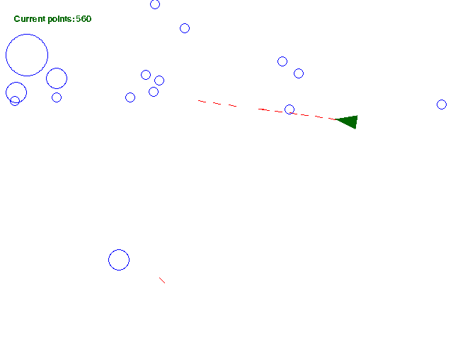
Figure 1: Screenshot of the asteroids game

The game itself involves a spaceship that can move around a 2D world and shoot bullets. Asteroids (depicted as circles) float around the world. The objective is to control the spaceship to shoot all of the asteroids, without being hit by an asteroid.

The game produces three kinds of percepts:

• see(Obj,Dir,Dist) - “the spaceship sees the object Obj in the direction Dir (left, right, centre or dead_centre) at a distance of Dist (pixels)”;

• facing_direction(RDir) - “the spaceship is currently facing in the direction RDir (measured in radians, where $0^{r}$ is east)”;

• speed(S) - “the spaceship is currently travelling with speed S”.

One see/3 percept is produced for every single thing the spaceship sees. In this game, the only thing that can be seen are asteroids. The number of see/3 percepts that are generated depends on how many asteroids are in the spaceship’s field of vision. It expected that a real robotic agent will not know the full state of the world, so it makes sense to restrict a simulated model’s knowledge as well, to demonstrate how teleo-reactive programming can operate on incomplete sensory information.

If the asteroids are almost directly in front of the space ship, then the Dir term of the percept will be dead_centre. If the asteroids are almost in front of the space ship, but not close enough to be dead_centre, the term will be center. If they are to the left or right (up to some angle) then the term will be left or right. So asteroids that are behind the spaceship will not be sensed. Asteroids that are more than 300 pixels away from the asteroid will also not be sensed. The space ship’s field of vision is illustrated in the diagram (Figure 2).

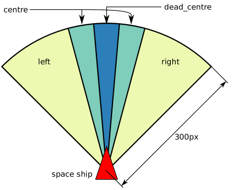
Figure 2: Diagram showing the behaviour of the see/3 percept

The actions that can be received by the program are:

• move_forward - move the space ship forward;

• move_backward - move the space ship backward;

• turn_left - turn the space ship left;

• turn_right - turn the space ship right;

• shoot - shoot.

All of these actions are durative, which means that one signal is sent to Pedro to indicate that the action is to start, then another one is sent when the action ends. This is to be contrasted with discrete actions, where one signal is sent to tell the agent to do the action.

Example programs

Every program for this demonstration has the same type definitions and declarations - these define the valid inputs and outputs. These are:

thing ::= asteroid | something_else
direction ::= left | right | centre | dead_centre

durative turn_right : (),
         turn_left : (),
         move_forward : (),
         move_backward : (),
         nothing : (),
         shoot : ()

percept facing_direction : (num),
        see : (thing, direction, num),
        speed : (num)

This defines two types: thing and direction. It also declares the types of six durative actions and three percepts. These are then referred to in the right hand side and left hand side of the rules, respectively. Procedures can now be written in terms of these percepts and actions.

The simplest procedure consists of one rule with a guard that is always inferable (true), which tells the agent (space ship) to do nothing. The procedure has no arguments and so has a type of (). Its is written:

proc1 : () ~>
proc1(){
true ~> ()
}

If the agent is to do anything, an action will have to be placed on the right hand side. This procedure tells the space ship to move forward, indefinitely:

proc2 : () ~>
proc2(){
true ~> move_forward
}

Now for a more advanced program. The verbose nature of this code was a result of a feature being accidentally missed out - the ability to put a conjunction of queries under a negation by failure statement (e.g. “q(a) & not (b(X) & c(X))”). inner_proc_left and inner_proc_right function as negation by failure statements.

proc3 : () ~>
proc3(){
see(asteroid, left, D) ~> inner_proc(D)
see(asteroid, right, D) ~> inner_proc(D)
true ~> move_forward
}

inner_proc : (num) ~>
inner_proc(D){
see(asteroid, left, D2) & D2 < D ~> inner_proc(D2)
see(asteroid, right, D2) & D2 < D ~> inner_proc(D2)
see(asteroid, left, D2) & D2 == D ~> turn_left, shoot
see(asteroid, right, D2) & D2 == D ~> turn_right, shoot
}

In this program, proc3 calls inner_proc with a numerical argument D which represents the current distance asteroid that has just been spotted (that is on the left or right of the space ship). inner_proc recursively calls itself until it has found the closest asteroid to the space ship (that is on the left or right of the space ship). Then, depending on the side, it tells the space ship to turn left or right and shoot. This is definitely not the best way to write this program, the intended meaning of the program was more like:

proc3 : () ~>
proc3(){
see(asteroid, left, Dist1) &
  not (see(asteroid,X,Dist2) & Dist2 < Dist1) ~> turn_left, shoot
see(asteroid, right, Dist1) &
  not (see(asteroid,X,Dist2) & Dist2 < Dist1) ~> turn_right, shoot
true ~> move_forward
}

This program is able to play Asteroids and win some games. It prioritises destroying the nearest asteroid. However, it sometimes exhibits strange behaviour because it does not take all information about the world into account. If an asteroid is travelling near the space ship and is about to pass it, the space ship may not be able to turn round quickly enough to aim at it. This sometimes causes it to miss.

Another situation that confounds this program is when there are multiple asteroids all at a similar distance from the space ship, the space ship will constantly be changing direction to aim at a different one. The result being that it does not succeed in aiming at any of them. One way to address this could be to set a small minimum limit on the amount of time that a rule can fire. This could be done by adding a “while min T” clause to the rule conditions, where T is a positive floating point number. No while condition is given, so it defaults to false. So the revised rules would look like this:

proc3 : () ~>
proc3(){
see(asteroid, left, Dist1) &
  not (see(asteroid,X,Dist2) &
  Dist2 < Dist1) while min 0.1 ~> inner_proc_left(Dist1)

see(asteroid, right, Dist1) &
  not (see(asteroid,X,Dist2) &
  Dist2 < Dist1) while min 0.1~> inner_proc_right(Dist1)
true ~> move_forward
}

Another program that could be written is one that maintains some percept, such as the speed of the space ship. The following program contains a procedure regulate_speed which takes a number as input and ensures that the space ship travels at that speed. It does so by speeding up when its speed drops below the level and doing nothing otherwise (the game world has some friction so the ship is inclined to slow down gradually). This example shows how self-regulating behaviour can be programmed.

proc4 : () ~>
proc4(){
true ~> regulate_speed(5)
}

regulate_speed : (num) ~>
regulate_speed(D){
speed(S) & S < D ~> move_forward
true ~> ()
}

3 Evaluation of the demonstration

The problem that I set out to investigate with teleo-reactive programming was that of developing robust, opportunistic programs to control robots in continuously varying environments. In this situation, a program is robust if it is able to recover from failures or setbacks. A program is opportunistic if it is able to take advantage of fortunate circumstances to more quickly achieve its goals. I do not believe that the Asteroids demo was sufficient to demonstrate that teleo-reactive programming was robust or opportunistic for these reasons:

To win at asteroids, the player has to do two things: shoot at asteroids and avoid being hit by asteroids. Unlike solving a puzzle, or performing a complex task, these tasks are not (obviously) made up of a high number of sub-tasks. If an agent is pursuing some strategy that is made up of one or two steps, if something happens to disrupt its behaviour, it will be set back at most one or two steps. This kind of robustness is simple enough that it can be hand-coded into a non-teleo-reactive program. In short, the Asteroids problem does not require a sufficiently hierarchical solution for it to be a good test of teleo-reactive programming.

That said, the Asteroids demo does demonstrate how easy it is to program applications that continuously react to the environment using teleo-reactive programming. For example, a procedure can be written in about eight lines (in a language that lets the programmer write negation of failure of conjunctions of predicates) that can play a game of Asteroids. Still, in order for this to be properly tested, a more complex example would need to be constructed.

2 Evaluation of my implementation

From the perspective of the user, my implementation of teleo-reactive programming has far fewer features than Qulog/TeleoR. Features that it lacks[Clark and Robinson, 2014a, b] include:

• The ability for the user to define their own functions and relations;

• The ability to execute tasks (procedures) in parallel;

• Communication with other teleo-reactive agents - communication is solely between the agent and its sensors / actuators;

• Timed sequences of action;

• Wait/repeat actions;

• Moded type declarations;

However, this does not entirely exclude it from being of use for simple tasks. Situations where feedback loops or reactive behaviour are required can be modelled in this application (as shown by the Asteroids example).

3 Practical considerations

This section concerns issues about the project that do not specifically correspond to teleo-reactive programming.

1 Why was Python used?

The TR algorithm stated in [Clark and Robinson, 2014b, a] formed the initial basis of the teleo-reactive system. I chose Python because it is the programming language I am most comfortable with and the fact that it is typically used as an imperative language meant that the TR algorithm easily translated to Python code. The choice of language was mostly a matter of personal preference.

Initially, I considered embedding Qulog in Haskell because simpler logic programming languages had already been successfully embedded in it[Claessen and Ljunglöf, 2000, Spivey and Seres, 1999]. This course of action was not taken in the end because it was agreed that it might not be feasible to embed enough of Qulog in Haskell to produce a complete working system in the time available.

2 Can the teleo-reactive system be compiled?

Python programs are typically run as interpreted programs, but can be converted to stand-alone executables that do not require Python to be installed to run. This can be done using a programs such as Pyinstaller[Various, 2015a] or py2exe[Various, 2015b]. The compiled program can then run on the computer controlling the robot, providing that it can run one of the operating systems supported by Pyinstaller/py2exe.

3 How does it scale?

No empirical analysis was done of the system’s scalability (i.e. by testing it on a very large input). With that said, some points where the program could be made more efficent were identified.

Redundancy when evaluating guard conditions - every time a single guard condition is queried, every predicate(percept/belief) in the BeliefStore is checked against it. Depending on the number of sensors, the amount of predicates (i.e. sensor data) in the BeliefStore could be very high. One solution is to use a relational database like MySQL or SQLite[MySQL, 1995, Hipp and Kennedy, 2007]. Every percept and belief could be represented by a table in the database. All of the variable instantiations for a single guard condition can be returned by a single SQL query.

Modifications to the teleo-reactive component of the system should also be considered. The optimisation described in Section 4 could be used to minimise the number of times that rules are re-evaluated, by only querying the relevant guard conditions. Another optimisation to consider is that of Mousavi and Broda [Mousavi and Broda, 2003], which offers methods for simplfying teleo-reactive sequences by removing redundant rules and literals.

4 Why did you write an interpreter?

The objective of this project was to explore teleo-reactive programming, rather than one into compiler design. Interpreters are easier to write than compilers because they do not involve a code generation step. Since code generation was not the aim of this project, the decision to write an interpreter was taken.

Another alternative to an interpreter is an embedding of the language. A “shallow embedding” of Qulog in Haskell was originally considered, along the lines of[Claessen and Ljunglöf, 2000, Spivey and Seres, 1999]. A shallow embedding is when the operations of the language (i.e. Qulog) are implemented in the host language (i.e. Python or Haskell). In the case of Qulog, this would be functions to perform logic programming (unification, resolution, search) for the guard conditions, evaluate TR procedures, functions and concurrency. There was no reason other than familiarity with the idea of writing interpreters and compilers that an interpreter was developed and not an embedding.

4 Other implementations of teleo-reactive programming

Many variations and extensions of the original TR language [Nilsson, 1994] have been developed over the years. A systematic review of teleo-reactive programming produced in 2014 provided references to most of the following papers[Morales et al., 2014]. The first one cited by [Morales et al., 2014] is [Lee and Durfee, 1994] which proposes a new circuit semantics Structured Circuit Semantics. This addresses some shortcomings with Nilsson’s original formalism:

• Execution Cycle - The paper proposes that because a teleo-reactive system as implemented on a computer works (at some level) in a discrete fashion, then durative (here called “energized”) actions should instead be treated as many discrete (or “ballistic”) actions. This makes no difference to the actual operation of the agent, so long as the perception-cognition-action frequency (i.e. the frequency of the main TR loop) is at or higher than the characteristic frequency of the system the agent is operating in.

• Non-Deterministic Behaviour - the original TR language requires the programmer to order the rules in a procedure strictly and statically (i.e. they must be in some order and the order cannot change mid-execution). Lee and Durfee’s modification allows the programmer to specify multiple “equally good” actions using a do any statement. This takes multiple rules and tries one non-deterministically. If it fails, it will try another one. If every rule fails then the whole rule fails.

• Best-First Behaviour - Sometimes, the best rules to consider (i.e, the order in which rules should be given) depends on some dynamically changing cost function. The modified language includes a do best statement that can contain multiple rules, each with a cost function. When such a statement is evaluated, the cost functions of each rule are evaluated and the condition/action pair of the one with the best cost function is then considered. This introduces an extra level of reasoning, which the paper called the “decision layer”.

• Failure Semantics - In SCS, every primitive action returns “success” or “failure” depending on whether it successfully had an effect on the world. These propagate upwards, for example if a group of actions are to be performed sequentially, then that group of actions will fail if any one of the actions fails. This success/fail message determines how do any and do best behave.

In addition to the above features, there are a few others such as parallel execution of steps, the do first structure (which chooses the first rule whose conditions are satisfied, much like in a TR program)[Lee and Durfee, 1994]. The syntax is also different to TR [Nilsson, 1994] and TeleoR [Clark and Robinson, 2014b].

In 1995, Zelek introduces TR+ , an extension to TR which lets actions be performed concurrently. The programmed agent was also able to perform dynamic real time path planning. TR+ was tested out on real life robots and software tools were developed to aid the development of TR+ applications: PVM, which allows TR+ programs to be run on a cluster of heterogenous computers (i.e. the computers do not have to be identical) and a program for displaying and manipulating TR+ programs as tree graphics[Zelek and Levine, 1995].

Nils Nilsson and Scott Sherwood Benson extended TR in [Benson and Nilsson, 1993] to allow the agent to work towards achieving multiple goals with different and time-varying urgencies, take advantage of a planning system to augment its own program and to change its program based on input from humans, successful/unsuccessful experiences and supervised/unsupervised training methods[Benson and Nilsson, 1993].

In 1996, Scott Sherwood Benson describes TRAIL (Teleo-Reactive Agent with Inductive Learning). It does so by recording its environment as it executes a plan or by observing a trainer. Then it identifies instances of action success or failure. Finally it uses a variant of the Inductive Logic Programming algorithm DINUS to induce action models (TR programs) based on the recorded data. This is applied to several problems domains: a 2D “Botworld” which involves a robot grabbing a bar, the “Delivery domain” where a robot has to navigate between rooms to perform some task and a flight simulator, where TRAIL was connected to an existing flight simulator[Benson, 1996].

In 2003, Mousavi and Broda describe a method for simplfying TR sequences. An algorithm is presented which, given a TR program, returns one that is smaller but semantically equal to the original. It does so by removing redundant rules (rules which will never be evaluated) and redundant literals (predicates that do not affect the result of the computation). It also shows how this method can be applied to simplify decision lists[Mousavi and Broda, 2003].

In 2008, Gubisch et al introduce an architecture based on teleo-reactive programming for control of mobile robots. This implementation translates the given TR program into C++ code, which can then be compiled by the g++ C++ compiler into a program that can be executed quickly by the robot. The paper describes how this was applied to control RoboCup (a robotic soccer competition) robots[Gubisch et al., 2008].

In 2014, Soto, Sánchez, Mateo, Alonso and Navarro developed an educational tool that converts teleo-reactive programs to VHDL, VHSIC Hardware Description Language. This language can then be used in programmable hardware devices, such as field programmable gate arrays (FPGAs)[Soto et al., 2014].

In 2012, Robert Kowalski and Fariba Sadri gave a semantics for teleo-reactive programs, expressed in terms of abductive logic programming (ALP). It compares the semantics to that of LPS (Logic-based Production System and agent language), another language that can also be expressed in terms of ALP[Kowalski and Sadri, 2012].

In summary, in addition to TeleoR[Clark and Robinson, 2014a, b], various other extensions of the original TR language have been proposed [Lee and Durfee, 1994, Zelek and Levine, 1995, Benson and Nilsson, 1993, Benson, 1996]. Various methods of implementing teleo-reactive programs have also been introduced, such as compiled C++ code[Gubisch et al., 2008], virtual hardware descriptions[Soto et al., 2014] and abductive learning[Kowalski and Sadri, 2012].

5 Alternatives to teleo-reactive programming

According to the paper [Dongol et al., 2014], the advantage that teleo-reactive programming provides over formalisms such as continuous action systems[Back et al., 2000, Meinicke and Hayes, 2006], TLA+[Lamport, 2002] and hybrid automata[Henzinger, 2000] is that it uses durative actions that specify a behaviour over time instead of instantaneous discrete actions. This and that fact that teleo-reactive programs have a hierarchical organisation means that the representations can be less complicated than the equivalent action system[Dongol et al., 2014].

One system that could perform a similar role to teleo-reactive programming is functional reactive programming (FRP). It can be used to describe hybrid systems - which are systems that combine both continuous and discrete components[Hudak et al., 2003]. FRP extends functional programming to allow programs where the outputs continuously react to their inputs to be written[Nilsson et al., 2002]. Several systems exist to allow this, such as Elm [Czaplicki, 2012] (used for creating web-based graphical user interfaces) and many Haskell libraries [HaskellWiki, 2015b].

Chapter 5 Conclusion & Future Work

This report has given a detailed background summary on two instances of teleo-reactive programming, TR and TeleoR. It has discussed the implementation issues associated with several of the features of those two systems. Concepts behind teleo-reactive programming were discussed, such as the triple and two tower architectures.

A teleo-reactive system was built in Python, modelled on TR and TeleoR. To demonstrate its effectiveness, it was used to control a simple video game, throug the Pedro communications architecture. The implementation of the teleo-reactive system was discussed, with regards to some of the design decisions made, such as those concerning typed expressions. Example programs were provided.

Future Work

If I had more time, I would have liked to implement concurrency in my application - Qulog provides one method but several other approaches have been discussed by others

To really demonstrate the utility of teleo-reactive programming, a more complex problem than “Asteroids” should be found. The problem should require a solution that is too complex for a single programmer to think about it in its entirety all at once. The “Asteroids” example was too simple, because the problem was small enough that a programmer could imagine the complete solution (programming an AI that wins the game by shooting all the asteroids) as one strategy. That said, “Asteroids” was a useful tool for debugging the Python implementation - I ensured that the simulation itself was stable by controlling it with Qulog, then replaced Qulog with my implementation.

Another aspect of teleo-reactive programming that should be better demonstrated is its robustness. A real-world demonstration would demonstrate this because of the complexity and unpredictable nature of the real world, compared to virtual worlds. A good place to start would be with the Robot Operating System (ROS), which is a modular collection of robotics software (nodes) and a communications protocol to connect those nodes together. It supports publish/subscribe messaging using “topics” that nodes can subscribe to and direct peer-to-peer communication using “services”[Quigley et al., 2009]. It also has a simulator, Gazebo, which means that control code can be tested out on a simulated robot and then run on a real life robot with the same physical attributes[Koenig and Howard, 2004].

Another area that would have been interesting to explore is a possible connection between teleo-reactive and functional reactive programming. Both of them concern outputs that vary depending on continuous input. Functional reactive programming has been used for robotics [Hudak et al., 2003].

References

- Nilsson [1994] NJ Nilsson. Teleo-reactive programs for agent control. JAIR, 1:139–158, 1994. URL http://www.jair.org/media/30/live-30-1375-jair.ps.Z.
- Nilsson [2001] NJ Nilsson. Teleo-reactive programs and the triple-tower architecture. Electron. Trans. Artif. Intell., 5(B):99–110, 2001. URL http://citeseerx.ist.psu.edu/viewdoc/download?doi=10.1.1.131.3833&rep=rep1&type=pdf.
- Clark and Robinson [2014a] K L Clark and P J Robinson. Programming Robotic Agents : A Teleo-Reactive Multi-Tasking Approach. 2014a.
- Clark and Robinson [2014b] KL Clark and PJ Robinson. Robotic Agent Programming in TeleoR. doc.ic.ac.uk, 2014b. URL http://www.doc.ic.ac.uk/~klc/ShortTeleoRIntro.pdf. [Online; accessed 03-09-2015].
- Nilsson [1992] NJ Nilsson. Toward Agent Programs With Circuit Semantics. 1992. URL http://ai.stanford.edu/users/nilsson/trweb/cktsem.pdf.
- Dongol et al. [2014] Brijesh Dongol, Ian J Hayes, and Peter J Robinson. Reasoning about goal-directed real-time teleo-reactive programs. Formal Aspects of Computing, 26(3):563–589, 2014.
- Kowalski and Sadri [2012] Robert A Kowalski and Fariba Sadri. Teleo-reactive abductive logic programs. In Logic Programs, Norms and Action, pages 12–32. Springer, 2012.
- Sergot [2010] Marek Sergot. Negation as failure (normal logic programs) (v1.3e), 2010. URL http://www.doc.ic.ac.uk/~mjs/teaching/KnowledgeRep491/NBF_491-2x1.pdf.
- Clark and Robinson [2015] K L Clark and P J Robinson. The Qulog/TeleoR 0.4 Reference Manual, 2015. URL http://staff.itee.uq.edu.au/pjr/HomePages/QulogFiles/manual/index.html. [Online; accessed 21-08-2015].
- [10] K L Clark and P J Robinson. QuLog : A flexibly typed logic based language with function and action rules. pages 1–17.
- Robinson [1965] J. A. Robinson. A machine-oriented logic based on the resolution principle. J. ACM, 12(1):23–41, January 1965. ISSN 0004-5411. 10.1145/321250.321253. URL http://doi.acm.org/10.1145/321250.321253.
- Martelli and Montanari [1976] Alberto Martelli and Ugo Montanari. Unification in linear time and space: A structured presentation. Istituto di Elaborazione della Informazione, Consiglio Nazionale delle Ricerche, 1976.
- Martelli and Montanari [1982] Alberto Martelli and Ugo Montanari. An efficient unification algorithm. ACM Trans. Program. Lang. Syst., 4(2):258–282, April 1982. ISSN 0164-0925. 10.1145/357162.357169. URL http://doi.acm.org/10.1145/357162.357169.
- Paterson and Wegman [1976] Michael S Paterson and Mark N Wegman. Linear unification. In Proceedings of the eighth annual ACM symposium on Theory of computing, pages 181–186. ACM, 1976.
- Robinson and Clark [2009] Peter J Robinson and Keith L Clark. Pedro : A publish / subscribe server using Prolog technology. pages 1–16, 2009.
- McGuire [2015] Paul McGuire. Pyparsing wiki, 2015. URL https://pyparsing.wikispaces.com. [Online; accessed 30-08-2015].
- Ranta [2011] Aarne Ranta. Lecture 7: Type checking, 2011. URL http://www.cse.chalmers.se/edu/year/2011/course/TIN321/lectures/proglang-07.html. [Online; accessed 30-08-2015].
- HaskellWiki [2015a] HaskellWiki. Type inference, 2015a. URL https://wiki.haskell.org/index.php?title=Type_inference&oldid=17047. [Online; accessed 01-09-2015].
- Webb [2015] Robert Webb. Asteroids game, 2015. URL https://github.com/rjwebb/asteroids.
- Morales et al. [2014] Jose Luis Morales, Pedro Sánchez, and Diego Alonso. A systematic literature review of the teleo-reactive paradigm. Artificial Intelligence Review, 42(4):945–964, 2014.
- Lee and Durfee [1994] Jaeho Lee and Edmund H Durfee. Structured circuit semantics for reactive plan execution systems. Ann Arbor, 1001:48109, 1994.
- Zelek and Levine [1995] John S Zelek and Martin D Levine. Teleo-reactive autonomous mobile navigation. In Electrical and Computer Engineering, 1995. Canadian Conference on, volume 1, pages 477–480. IEEE, 1995.
- Benson and Nilsson [1993] Scott Benson and Nils J Nilsson. Reacting, planning, and learning in an autonomous agent. In Machine intelligence 14, pages 29–64. Citeseer, 1993.
- Benson [1996] Scott Sherwood Benson. Learning action models for reactive autonomous agents. PhD thesis, stanford university, 1996.
- Mousavi and Broda [2003] Seyed R Mousavi and Krysia Broda. Simplification Of Teleo-Reactive sequences. Imperial College of Science, Technology and Medicine, Department of Computing, 2003.
- Gubisch et al. [2008] Gerhard Gubisch, Gerald Steinbauer, Martin Weiglhofer, and Franz Wotawa. A teleo-reactive architecture for fast, reactive and robust control of mobile robots. In New Frontiers in Applied Artificial Intelligence, pages 541–550. Springer, 2008.
- Soto et al. [2014] Fulgencio Soto, Pedro Sánchez, Antonio Mateo, Diego Alonso, and Pedro J Navarro. An educational tool for implementing reactive systems following a goal-driven approach. Computer Applications in Engineering Education, 22(4):764–773, 2014.
- Back et al. [2000] R-J Back, Luigia Petre, and Ivan Porres. Generalizing action systems to hybrid systems. In Formal Techniques in Real-Time and Fault-Tolerant Systems, pages 202–213. Springer, 2000.
- Meinicke and Hayes [2006] Larissa Meinicke and Ian J Hayes. Continuous action system refinement. In Mathematics of Program Construction, pages 316–337. Springer, 2006.
- Lamport [2002] Leslie Lamport. Specifying systems: the TLA+ language and tools for hardware and software engineers. Addison-Wesley Longman Publishing Co., Inc., 2002.
- Henzinger [2000] Thomas A Henzinger. The theory of hybrid automata. Springer, 2000.
- Hudak et al. [2003] Paul Hudak, Antony Courtney, Henrik Nilsson, and John Peterson. Arrows, robots, and functional reactive programming. In Advanced Functional Programming, pages 159–187. Springer, 2003.
- Nilsson et al. [2002] Henrik Nilsson, Antony Courtney, and John Peterson. Functional reactive programming, continued. In Proceedings of the 2002 ACM SIGPLAN workshop on Haskell, pages 51–64. ACM, 2002.
- Czaplicki [2012] Evan Czaplicki. Elm: Concurrent frp for functional guis. Senior thesis, Harvard University, 2012.
- HaskellWiki [2015b] HaskellWiki. Functional reactive programming - haskellwiki, 2015b. URL https://wiki.haskell.org/index.php?title=Functional_Reactive_Programming&oldid=60037. [Online; accessed 03-09-2015].
- Claessen and Ljunglöf [2000] K Claessen and Peter Ljunglöf. Typed Logical Variables in Haskell. Electr. Notes Theor. Comput. Sci., 41(1):37, 2000. URL http://citeseerx.ist.psu.edu/viewdoc/download?doi=10.1.1.37.2565&rep=rep1&type=pdf.
- Spivey and Seres [1999] JM Spivey and Silvija Seres. Embedding Prolog in Haskell. Proceedings of Haskell, pages 1–14, 1999. URL http://www.researchgate.net/profile/Silvija_Seres/publication/2592935_Embedding_PROLOG_in_HASKELL/links/09e4150de391feb21e000000.pdf.
- Various [2015a] Various. pyinstaller, 2015a. URL https://github.com/pyinstaller/pyinstaller/wiki.
- Various [2015b] Various. py2exe, 2015b. URL http://www.py2exe.org/.
- MySQL [1995] AB MySQL. MySQL: the world’s most popular open source database. MySQL AB, 1995.
- Hipp and Kennedy [2007] D Richard Hipp and D Kennedy. Sqlite, 2007.
- Quigley et al. [2009] Morgan Quigley, Ken Conley, Brian Gerkey, Josh Faust, Tully Foote, Jeremy Leibs, Rob Wheeler, and Andrew Y Ng. Ros: an open-source robot operating system. In ICRA workshop on open source software, volume 3, page 5, 2009.
- Koenig and Howard [2004] Nathan Koenig and Andrew Howard. Design and use paradigms for gazebo, an open-source multi-robot simulator. In Intelligent Robots and Systems, 2004.(IROS 2004). Proceedings. 2004 IEEE/RSJ International Conference on, volume 3, pages 2149–2154. IEEE, 2004.