Pancharatnam Phase Deficit can detect Macroscopic Entanglement

Abstract

The Pancharatnam phase deficit is defined as the difference between the Pancharatnam phase acquired by the global system and sum of the Pancharatnam phases acquired by subsystems during local unitary evolutions. We show that a non-zero value of the Pancharatnam phase deficit for a composite quantum system can be a signature of quantum entanglement. In the context of macroscopic quantum systems, we illustrate how the Pancharatnam phase deficit can be used to detect macroscopically entangled states. In particular, we use the Pancharatnam phase deficit to detect the entanglement for macroscopic superposition of coherent states. Furthermore, we show that by measuring the Pancharatnam phase deficit one can measure the concurrence of two spin singlets between distant boundaries.

1 Introduction

Berry’s phase, alternatively called as the Panchratnam phase [1] has been a subject of great importance in quantum mechanics. The Barry phase has been generalized for non adiabatic but cyclic evolutions of quantum system [2] and for noncyclic evolutions [3]. In general, without taking into account the initial ideas of adiabaticity, cyclicity, and unitarity for geometric phase, if a quantal system undergoes an evolution, we can can compute the phase difference in the process of evolution by the inner product between the states before and after evolution, with an exception of initial and final states being orthogonal [4, 5]. The geometric phase has been studied for various quantum systems [6, 7, 8] and it has important applications [9, 10, 11, 12, 13, 15, 16, 17, 14, 18] in literature.

Quantum entanglement [19, 20] being at the heart of quantum information theory, its detection plays very important role in quantum systems. The connection of geometric phase and entanglement has also been studied before [21, 22, 23] and the noncyclic geometric phase for entangled states was calculated by Sjöqvist [24]. Since, in principle, quantum mechanics may permit the existence of a macroscopic object which is in a quantum superposition, it has become very important to study the macroscopic quantumness and macroscopic entanglement. Macroscopic quantumness is one of the crucial aspects of the present research on quantum systems and it is strongly connected with the quantum to classical transition and the measurement problem [21]. There have been several proposals to quantify macroscopicity based on different criteria involving effective number of particles in the superposition states, dishtinguishability and operational interpretations [25, 26, 27, 28]. In recent years, macroscopic quantum states have been proposed in various systems such as superconductors [29, 30, 31, 32], nanoscale qubits [33, 34], trapped ions [35], and photonic qubits in microwave cavity [36]. Constructing such macroscopically superposed states [37, 38], studying and detecting entanglement in such macroscopic states are need of the hour to understand the extent of applicability of quantum mechanics.

In this letter we make use of the notion of the Pancharatnam phase deficit during arbitrary local unitary evolution of a macroscopic quantum system and show how one can detect entanglement using the Pancharatnam phase deficit. A bipartite pure quantum system, subjected to local unitary evolution acquires a Pancharatnam phase during the evolution. However, the individual subsystems also acquire their respective Pancharatnam phases during the evolution. We show that if the state is separable, then the difference in the global Pancharatnam phase and sum of the local Pancharatnam phases, which we call as the Pancharatnam phase deficit, will be zero. Therefore, a nonzero value of the Pancharatnam phase deficit acquired by the pure composite system is a signature of entanglement. We show how the Pancharatnam phase deficit can be a signature of entanglement in macroscopic superposition of quantum states. Interestingly, in some specific examples, we show that the entropy of entanglement and concurrence for macroscopic system can be expressed solely using the Pancharatnam phase deficit.

2 Pancharatnam Phase Deficit for Bipartite States

Consider an arbitrary initial product state $|\Psi(0)\rangle_{AB}=|\psi(0)\rangle_{A}\otimes|\phi(0)\rangle_{B}\in{\cal H}_{A}\otimes{\cal H}_{B}$ of a bipartite composite system. Let this evolve under local unitary evolution, namely, the system is subject to Hamiltonian of the form $H=H_{A}\otimes I+I\otimes H_{B}$. Under the action of the Hamiltonian the state evolves unitarily as $|\Psi(0)\rangle_{AB}\rightarrow|\Psi(t)\rangle_{AB}=U(t)\ket{\psi(0)}_{A}\otimes V(t)\ket{\phi(0)}_{B}$, where $U(t)=e^{-iH_{A}t/\hbar}$ and $V(t)=e^{-iH_{B}t/\hbar}$. In this section we consider the local unitary evolution of a bipartite state and try to characterize the entanglement in terms of the difference of the Pancharatnam phases acquired by the system in global and local scenarios. The Pancharatnam phase acquired by the composite system is given by

$$\Phi_{T}^{AB} = Arg(\langle\Psi(0)|\Psi(t)\rangle).$$ (1)

Now, the Pancharatnam phases acquired by the subsystem $A$ and $B$, respectively, are given by

$$\Phi_{T}^{A}=Arg(\langle\psi(0)|\psi(t)\rangle),~{}\Phi_{T}^{B}=Arg(\langle\phi(0)|\phi(t)\rangle).$$ (2)

The Pancharatnam phase deficit is defined as the difference of the Pancharatnam phase acquired by the composite system and the sum of the Pancharatnam phases acquired by the local subsystems, i.e.,

$$\Delta = \Phi_{T}^{AB}-[\Phi_{T}^{A}+\Phi_{T}^{B}].$$ (3)

For product states, the Pancharatnam phase deficit is identically zero. Therefore, if it is nonzero, then the state will be entangled. Hence, a non-zero Pancharatnam phase deficit is shown to be a signature of entanglement in the composite quantum system.

Suppose we have a general bipartite state in $\cal H_{A}^{\text{\it N}}\otimes\cal H_{B}^{\text{\it M}}$ for the composite system. Using the Schmidt decomposition theorem we can write the combined bipartite state (with $N<M$) as

$$|\Psi\rangle_{AB}=\sum_{n=1}^{N}\sqrt{\lambda_{n}}|a_{n}\rangle|b_{n}\rangle,$$ (4)

where $\lambda_{n}$’s are the Schmidt coefficients with $\sum_{n}\lambda_{n}=1$, $|a_{n}\rangle\in{\cal H}_{A}$ and $|b_{n}\rangle\in{\cal H}_{B}$ are the orthonormal Schmidt basis. Let the state evolve as $|\Psi\rangle_{AB}\rightarrow U(t)\otimes V(t)|\Psi\rangle_{AB}$. Under this local unitary evolution, the Pancharatnam phase for the composite state is given by

$$\Phi_{T}^{AB} = Arg(\langle\Psi|U(t)\otimes V(t)\Psi\rangle).$$ (5)

To find the Pancharatnam phases for subsystems, we have to recourse to the notion of the mixed state Pancharatnam phase [18]. For the subsystems $A$ and $B$ this is given by

$$\Phi_{T}^{A}=Arg(Tr[\rho_{A}U(t)]),~{}\Phi_{T}^{B}=Arg(Tr[\rho_{B}V(t)]).$$ (6)

Therefore, for a general bipartite entangled state the Pancharatnam phase deficit is given by

$$\Delta = \Phi_{T}^{AB}-[\Phi_{T}^{A}+\Phi_{T}^{B}]$$

$$= \tan^{-1}\big{[}\frac{\sum_{kl}\sqrt{\lambda_{k}\lambda_{l}}(ImU_{kl}ReV_{kl}+ReU_{kl}ImV_{kl})}{\sum_{kl}\sqrt{\lambda_{k}\lambda_{l}}(ReU_{kl}ReV_{kl}-ImU_{kl}ImV_{kl})}\big{]}$$

$$-\tan^{-1}\big{[}\frac{\sum_{k}\lambda_{k}ImU_{kk}}{\sum_{k}\lambda_{k}ReU_{kk}}\big{]}-\tan^{-1}\big{[}\frac{\sum_{k}\lambda_{k}ImV_{kk}}{\sum_{k}\lambda_{k}ReV_{kk}}\big{]},$$

where $U_{kl}=\langle a_{k}|U|a_{l}\rangle,$ and $V_{kl}=\langle b_{k}|V|b_{l}\rangle$. Note that for entangled state under local unitary evolutions, the global dynamical phase is equal to the sum of local dynamical phases for the subsystems $A$ and $B$, i.e., $\Phi_{D}^{AB}=\Phi_{D}^{A}+\Phi_{D}^{B}$. Hence, if one defines the dynamical phase deficit that will be always zero for entangled as well as separable states. Therefore, dynamical phase deficit cannot detect entanglement of bipartite states. It is the Pancharatnam phase that captures the notion of entangled state via a non-zero Pancharatnam phase deficit.

In the present method, we can detect entanglement without state tomography or measuring the spin observables. Also our method can detect entanglement and measure the entropy of entanglement for two spin half particles using the Pancharatnam phase deficit. Since we do not need cyclic or adiabatic conditions for the Pancharatnam phase deficit, our proposal is more general. Our result can be applied to detect entanglement across microscopic-microscopic as well as microscopic-macroscopic system partitions. For example, one can imagine that the subsystem $A$ is made of large number of elementary sub-sub systems (say $N\sim 10^{4}$) and the multiparticle states are orthonormal and have macroscopically distinct average value of a physical quantity. Such systems can also be imagined with quantum simulators [39] which will be able to emulate a large number of quantum systems and can exhibit quantum properties being a quantum system itself.

3 Pancharatnam Phase Deficit for Multi-particles

Suppose, we have a multi-particle state which is not in a product state. Then, let it undergo local unitary evolutions, i.e., $\ket{\Psi}_{A_{1}A_{2}....A_{N}}\rightarrow U_{1}\otimes U_{2}\otimes\cdots U_{N}\ket{\Psi}_{A_{1}A_{2}....A_{N}}$. The Pancharatnam phase acquired by the composite state is given by

$$\Phi_{T}^{A_{i}..A_{N}}=Arg(\langle\Psi|U_{1}\otimes U_{2}\otimes\cdots U_{N}\ket{\Psi}_{A_{1},A_{2}....A_{N}},$$ (8)

However, the constituent systems would also acquire their respective Pancharatnam phases during local evolutions and we denote them by $\Phi_{T}^{A_{i}}$, where $A_{i}=A_{1},A_{2},\ldots A_{N}$. The local Pancharatnam phase is given by

$$\Phi_{T}^{A_{i}}=Arg(Tr[\rho_{A_{i}}U_{i}]),$$ (9)

where $i=1,2,\ldots N$. The Pancharatnam phase deficit for $N$ particle is given by

$$\Delta = \Phi_{T}^{A_{i}..A_{N}}-\bigg{[}\sum_{i}\Phi_{T}^{A_{i}}\bigg{]}$$ (10)

$$= Arg(\bra{\Psi}|U_{1}\otimes U_{2}\otimes\cdots U_{N}\ket{\Psi}_{A_{1},A_{2}....A_{N}})$$

$$-\sum_{i}Arg(Tr[\rho_{A_{i}}U_{i}])$$

If $N$-particle state is a pure product state, then $\Delta=0$. This implies that a non-zero $\Delta$ signifies that the state $\Psi_{A_{1}A_{2}\ldots A_{N}}$ is entangled.

Our method can be applied to detect entangled states in quantum interferometry. In Mach-Zehnder interferometer set up, we can measure the relative phase acquired during the local unitary evolution by the global system and the local subsystems. Relative phase being easier to measure in interferometry, this is a convenient method to detect entanglement in composite systems. Whether our method of detecting entanglement using the Pancharatnam phase deficit is robust for decoherence, will be explored in future. It should be stressed that the explorations in macroscopic quantum systems is strongly related with the quantum to classical transition and the measurement problem. For example, it has been shown the existence of the environment which usually causes decoherence, can induce the Berry phase and entanglement between the system and the environment can be measured with the help of the Barry phase [40, 41].

4 Pancharatnam Phase Deficit for Entangled Macroscopic and Microscopic Systems

Using the single photon quantum-injected optical parametric amplification, the entanglement between the microscopic qubit and the macroscopic part has been obtained experimentally [42]. The macroscopic part consists of large number of photons. Below, we show how our result can be applied to detect the micro-macro entangled state. Consider a system composed of macroscopic and microscopic parts in an entangled state [42] such as,

$$|\Psi\rangle_{AB}=\sqrt{\lambda_{0}}~{}|\psi\rangle\otimes|0\rangle+\sqrt{\lambda_{1}}~{}|\bar{\psi}\rangle\otimes|1\rangle,$$ (11)

where the subsystem $A$ is a macroscopic quantum system (contains photon number of the order $10^{4}$) with $|\psi\rangle$, $|\bar{\psi}\rangle$ are the mutually orthogonal multiparticle macroscopic state (See for details [42]) and the subsystem $B$ is a microscopic system. Let the system evolve under local time-independent Hamiltonian

$$H=\epsilon_{1}|\bar{\psi}\rangle\langle\bar{\psi}|\otimes I_{B}+\epsilon_{2}I_{A}\otimes|1\rangle\langle 1|,$$ (12)

where $\epsilon_{1},\epsilon_{2}>0$ and $I_{A},I_{B}$ are the identity operators on $\cal H_{A}$ and $\cal H_{B}$. Under this Hamiltonian, the state $|\Psi\rangle_{AB}$ undergoes local unitary evolution given by $|\Psi\rangle_{AB}\rightarrow U\otimes V|\Psi\rangle$ and the evolved state is

$$|\Psi\rangle_{AB}(t) = e^{-i\epsilon_{1}t/\hbar|\bar{\psi}\rangle\langle\bar{\psi}|}\otimes e^{-i\epsilon_{2}t/\hbar|1\rangle\langle 1|}|\Psi\rangle_{AB}$$

$$= \sqrt{\lambda_{0}}~{}|\psi\rangle\otimes|0\rangle+\sqrt{\lambda_{1}}~{}e^{-i(g_{1}+g_{2})}|\bar{\psi}\rangle|1\rangle,$$

where $g_{1}=\epsilon_{1}t/\hbar$ and $g_{2}=\epsilon_{2}t/\hbar$. We have used the unitary evolution operators as

$$U = e^{-i\epsilon_{1}t/\hbar|\bar{\psi}\rangle\langle\bar{\psi}|}=(I-|\bar{\psi}\rangle\langle\bar{\psi}|)+e^{-i\epsilon_{1}t/\hbar}|\bar{\psi}\rangle\langle\bar{\psi}|,$$

$$V = e^{-i\epsilon_{1}t/\hbar|1\rangle\langle 1|}=(I-|1\rangle\langle 1|)+e^{-i\epsilon_{1}t/\hbar}|1\rangle\langle 1|.$$ (14)

The Pancharatnam phase acquired by the composite system during this evolution turns out to be

$$\Phi_{T}^{AB}=tan^{-1}\bigg{[}\frac{-\lambda_{1}\sin(\epsilon_{1}+\epsilon_{2})t/\hbar}{\lambda_{0}+\lambda_{1}\cos(\epsilon_{1}+\epsilon_{2})t/\hbar}\bigg{]}.$$ (15)

The local Pancharatnam phase shifts are given by

$$\Phi_{T}^{A} = tan^{-1}\bigg{[}\frac{-\lambda_{1}\sin\epsilon_{1}t/\hbar}{1+\lambda_{1}(\cos\epsilon_{1}t/\hbar-1)}\bigg{]},$$ (16)

$$\Phi_{T}^{B} = tan^{-1}\bigg{[}\frac{-\lambda_{1}\sin\epsilon_{2}t/\hbar}{1+\lambda_{1}(\cos\epsilon t_{2}/\hbar-1)}\bigg{]}.$$ (17)

Therefore, the Pancharatnam phase deficit is given by

$$\Delta = \tan^{-1}\bigg{[}\frac{-\lambda_{1}\sin(\epsilon_{1}+\epsilon_{2})t/\hbar}{\lambda_{0}+\lambda_{1}\cos(\epsilon_{1}+\epsilon_{2})t/\hbar}\bigg{]}$$ (18)

$$-\tan^{-1}\bigg{[}\frac{-\lambda_{1}\sin\epsilon_{1}t/\hbar}{1+\lambda_{1}(\cos\epsilon_{1}t/\hbar-1)}\bigg{]}$$

$$-\tan^{-1}\bigg{[}\frac{-\lambda_{1}\sin\epsilon_{2}t/\hbar}{1+\lambda_{1}(\cos\epsilon t_{2}/\hbar-1)}\bigg{]}.$$

Now, if we choose the parameters in the Hamiltonian such that $\epsilon_{1}=\epsilon_{2}$ and $2\epsilon t/\hbar=\pi$, then we get

$$\lambda_{0}=\frac{1}{1+\tan\Delta/2},~{}\lambda_{1}=\frac{\tan\Delta/2}{1+\tan{\Delta/2}}.$$ (19)

The entropy of entanglement between the macroscopic and microscopic parts for this system is given by $E_{N}=-Tr(\rho_{A}\ln\rho_{A})=-Tr(\rho_{B}\ln\rho_{B})$. On using Eqs. (19) in this expression, we can express the entanglement entropy solely in terms of the Pancharatnam phase deficit. This is given by

$$E_{N} = -\frac{1}{1+\tan\Delta/2}\ln\Big{(}\frac{1}{1+\tan\Delta/2}\Big{)}$$ (20)

$$-\frac{\tan\Delta/2}{1+\tan\Delta/2}\ln\Big{(}\frac{\tan\Delta/2}{1+\tan\Delta/2}\Big{)}.$$

Thus, by suitably choosing the parameters in the Hamiltonian, one can directly measure the entanglement with the help of the Pancharatnam phase deficit in quantum interferometry.

5 Pancharatnam Phase deficit for macroscopic superposition of coherent states

Liu et al. [37] have proposed the generation of superposition of macroscopically distinguishable coherent states using a microwave cavity with a superconducting charge qubit. The evolved entangled state at time $t$ generated can be written in the form

$$|\Psi(t)\rangle_{AB}=\frac{1}{\sqrt{2}}\big{(}k|\alpha_{-}\rangle|g\rangle+k^{*}|\alpha_{+}\rangle|e\rangle\big{)},$$ (21)

where $k=e^{-i\bm{\psi}}$ is a complex constant with $\bm{\psi}=$ Im$\Big{[}\frac{\zeta E_{J}}{\hbar\omega}\alpha^{\prime}(1-e^{i\omega t})\Big{]}$ such that $\Omega=\zeta^{*}E_{J}/\hbar$ is complex Rabi frequency (see for details [37]). The injected coherent field $|\alpha^{\prime}\rangle$ has real amplitude $\alpha^{\prime}$ and $\omega$ is the frequency of single mode cavity field. $|g\rangle$ and $|e\rangle$ denote the ground state and the excited state of the atom, respectively. In order to test the entanglement in this given system, let this state evolve under $U\otimes V$ with $U$ and $V$ chosen as phase shifting operator and Pauli spin operator $U=e^{-i\theta\hat{N}}$ and $V=\sigma_{x}$, respectively. Here, $\hat{N}$ is number operator and $\sigma_{x}$ is the Pauli matrix. The transition amplitude under local evolution of the entangled state in Eq.(21) is given by

$$Tr[\rho_{AB}(t)U\otimes V]$$

$$=\frac{1}{2}\exp\big{(}-1/2(|\alpha_{-}|^{2}+|\alpha_{+}|^{2})\big{)}$$

$$\Big{[}\Big{(}k^{2}\exp\big{(}|\alpha_{-}||\alpha_{+}|\cos(\xi-\theta)\big{)}\cos\big{(}|\alpha_{-}||\alpha_{+}|\sin(\xi-\theta)\big{)}$$

$$+k^{*2}\exp\big{(}|\alpha_{-}||\alpha_{+}|\cos(\xi+\theta)\big{)}\cos\big{(}|\alpha_{-}||\alpha_{+}|\sin(\xi+\theta)\big{)}\Big{)}$$

$$+i\Big{(}k^{2}\exp\big{(}|\alpha_{-}||\alpha_{+}|\cos(\xi-\theta)\big{)}\sin\big{(}|\alpha_{-}||\alpha_{+}|\sin(\xi-\theta)\big{)}$$

$$-k^{*2}\exp\big{(}|\alpha_{-}||\alpha_{+}|\cos(\xi+\theta)\big{)}\sin\big{(}|\alpha_{-}||\alpha_{+}|\sin(\xi+\theta)\big{)}\Big{)}\Big{]},$$

(22)

on using the notations $\xi=\chi_{1}-\chi_{2}$, and $\alpha_{-}=|\alpha_{-}|e^{i\chi_{1}},~{}\alpha_{+}=|\alpha_{+}|e^{i\chi_{2}}$. The local phases acquired during this unitary evolution by the individual quantum systems can be given by

$$Tr[\rho_{A}(t)U]$$

$$=\frac{1}{2}\Big{[}\Big{(}\exp(|\alpha_{-}|^{2}(\cos\theta-1))\cos(|\alpha_{-}|^{2}\sin\theta)$$

$$+\exp(|\alpha_{+}|^{2}(\cos\theta-1)\cos(|\alpha_{+}|^{2}\sin\theta)\Big{)}$$

$$-i\Big{(}\exp(|\alpha_{-}|^{2}(\cos\theta-1))\sin(|\alpha_{-}|^{2}\sin\theta)$$

$$+\exp(|\alpha_{+}|^{2}(\cos\theta-1)\sin(|\alpha_{+}|^{2}\sin\theta)\Big{)}\Big{]},$$ (23)

$$Tr[\rho_{B}(t)V]$$

$$=\frac{1}{2}\exp\big{(}-1/2(|\alpha_{-}|^{2}+|\alpha_{+}|^{2})+|\alpha_{-}||\alpha_{+}|\cos\xi\big{)}$$

$$\Big{[}(k^{2}+k^{*2})\cos(|\alpha_{-}||\alpha_{+}|\sin\xi)$$

$$+i(k^{2}-k^{*2})\sin(|\alpha_{-}||\alpha_{+}|\sin\xi)\Big{]}.$$ (24)

Eq. (LABEL:difference_bipartite) gives the Pancharatnam phase deficit for this entangled state after unitary evolution as

$$tan^{-1}\left[\frac{\begin{multlined}\Big{(}k^{2}\exp\big{(}n\cos(\xi-\theta)\big{)}\sin\big{(}n\sin(\xi-\theta)\big{)}\\ -k^{*2}\exp\big{(}n\cos(\xi+\theta)\big{)}\sin\big{(}n\sin(\xi+\theta)\big{)}\Big{)}\end{multlined}\Big{(}k^{2}\exp\big{(}n\cos(\xi-\theta)\big{)}\sin\big{(}n\sin(\xi-\theta)\big{)}\\ -k^{*2}\exp\big{(}n\cos(\xi+\theta)\big{)}\sin\big{(}n\sin(\xi+\theta)\big{)}\Big{)}}{\begin{multlined}\Big{(}k^{2}\exp\big{(}n\cos(\xi-\theta)\big{)}\cos\big{(}n\sin(\xi-\theta)\big{)}\\ +k^{*2}\exp\big{(}n\cos(\xi+\theta)\big{)}\cos\big{(}n\sin(\xi+\theta)\big{)}\Big{)}\end{multlined}\Big{(}k^{2}\exp\big{(}n\cos(\xi-\theta)\big{)}\cos\big{(}n\sin(\xi-\theta)\big{)}\\ +k^{*2}\exp\big{(}n\cos(\xi+\theta)\big{)}\cos\big{(}n\sin(\xi+\theta)\big{)}\Big{)}}\right]$$ (29)

$$-tan^{-1}\left[\frac{\begin{multlined}\Big{(}-\exp(n_{-}(\cos\theta-1))\sin(n_{-}\sin\theta)\\ -\exp(n_{+}(\cos\theta-1)\sin(n_{+}\sin\theta)\Big{)}\end{multlined}\Big{(}-\exp(n_{-}(\cos\theta-1))\sin(n_{-}\sin\theta)\\ -\exp(n_{+}(\cos\theta-1)\sin(n_{+}\sin\theta)\Big{)}}{\begin{multlined}\Big{(}\exp(n_{-}(\cos\theta-1))\cos(n_{-}\sin\theta)\\ +\exp(n_{+}(\cos\theta-1)\cos(n_{+}\sin\theta)\Big{)}\end{multlined}\Big{(}\exp(n_{-}(\cos\theta-1))\cos(n_{-}\sin\theta)\\ +\exp(n_{+}(\cos\theta-1)\cos(n_{+}\sin\theta)\Big{)}}\right]$$ (34)

$$-tan^{-1}\Big{[}\frac{(k^{2}+k^{*2})\sin(n\sin\xi)}{(k^{2}-k^{*2})\cos(n\sin\xi)}\Big{]},$$

where $n_{-}=|\alpha_{-}|^{2},n_{+}=|\alpha_{+}|^{2}$ and $\sqrt{n_{-}n_{+}}=n$. To compare with the other measures of entanglement, we calculate the entropy of entanglement for this state as

$$E_{N} = -Tr(\rho_{A}\ln\rho_{A})$$

$$= \frac{1}{2\ln 2}\Big{(}kk^{*}e^{\frac{-n_{-}}{2}\frac{-n_{+}}{2}+n_{-}n_{+}\cos\xi}-1\Big{)}$$

$$\ln\Big{[}\frac{1}{2}\Big{(}1-kk^{*}e^{\frac{-n_{-}}{2}\frac{-n_{+}}{2}+n_{-}n_{+}\cos\xi}\Big{)}\Big{]}$$

$$-\frac{1}{2\ln 2}\Big{(}1+kk^{*}e^{\frac{-n_{-}}{2}\frac{-n_{+}}{2}+n_{-}n_{+}\cos\xi}\Big{)}$$

$$\ln\Big{[}\frac{1}{2}\Big{(}1+kk^{*}e^{\frac{-n_{-}}{2}\frac{-n_{+}}{2}+n_{-}n_{+}\cos\xi}\Big{)}\Big{]}$$

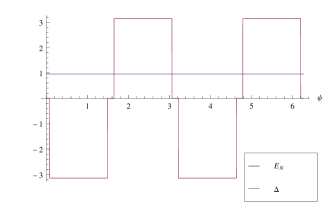
Figure 1: (Color Online) Variation of the Pancharatnam phase deficit $\Delta$ and entropy of entanglement $E_{N}$ with $\bm{\psi}$ for $|\alpha_{-}|^{2}=2,|\alpha_{+}|^{2}=1,~{}\xi=\pi/4$ and $\theta=\pi$.The blue line indicates the entropy of entanglement and the magenta line indicates the value of Pancharatnam phase deficit.

Now, we plot the entropy of entanglement and the Pancharatnam phase deficit for some specific values of parameters and very small photon numbers in the two coherent modes in Fig. 1. It is evident from the illustration that the non zero phase deficit is a sufficient condition for entanglement in a macroscopic quantum system.

6 Pancharatnam Phase deficit for two distant boundary spins

Bayat et al. [38] have proposed a method to create high entanglement between very distant boundary spins which is generated by suddenly connecting two long Kondo spin chains. As an example, they consider two spin singlets each formed by only two spins interacting with a Heisenberg interaction of strength $J_{1}$ and $J_{2}$, respectively. One may generate high entanglement between the boundary spins 1 and 4, by just turning on an interaction $J_{m}$ between the two spins 2 and 3. On choosing a specific condition $J_{m}=J_{1}+J_{2}$ at certain time, the evolved state at time $t$ (up to a global phase) for boundary spins 1 and 4 of the system, is given by

$$|\Psi(t)\rangle_{1234}=\frac{-i\sin(2J_{m}t)}{2}\big{(}|0011\rangle+|1100\rangle\big{)}-\frac{\cos(2J_{m}t)}{2}$$

$$\times\big{(}|1001\rangle+|0110\rangle\big{)}+\frac{e^{i2J_{m}t}}{2}\big{(}|0101\rangle+|1010\rangle\big{)}.$$

(36)

The concurrence $E$ [43] for spins 1 and 4 is given by

$$E=\max\bigg{\{}0,\frac{1-3\cos(4J_{m}t)}{4}\bigg{\}}.$$ (37)

Using the method discussed in this paper, we would see that not only the entanglement can be detected by nonzero phase deficit but the maximum phase deficit reflects the maximum entanglement. For the state given by Eq. (36) we choose the local unitary evolution under the following Hamiltonian in order to connect the entanglement between the spins 1 and 4 and the Pancharatnam phase deficit. The Hamiltonian is given by

$$H=\epsilon_{1}|1\rangle\langle 1|\otimes I_{2}\otimes I_{3}\otimes I_{4}+I_{1}\otimes I_{2}\otimes I_{3}\otimes\epsilon_{4}|1\rangle\langle 1|,$$ (38)

where $\epsilon_{1},\epsilon_{4}>0$ and $I_{1},I_{2},I_{3}$ and $I_{4}$ are the identity operators. Under this Hamiltonian, the state $|\Psi(t)\rangle$ undergoes local unitary evolution for another time $\tau$ as given by

$$|\Psi(t)\rangle_{1234}\rightarrow U_{1}\otimes I_{2}\otimes I_{3}\otimes U_{4}|\Psi(t)\rangle_{1234}$$

$$=e^{-i{\epsilon_{1}\tau/\hbar|1\rangle\langle 1|}}\otimes I_{2}\otimes I_{3}\otimes e^{-i{\epsilon_{4}\tau/\hbar|1\rangle\langle 1|}}|\Psi(t)\rangle_{1234}$$

(39)

This state after evolution can be written as

$$|\Psi^{{}^{\prime}}\rangle_{1234} = \frac{-i\sin(\theta)}{2}\bigg{\{}e^{-i\epsilon_{4}\tau/\hbar}|0011\rangle+e^{-i\epsilon_{1}\tau/\hbar}|1100\rangle\bigg{\}}$$ (40)

$$-\frac{\cos(\theta)}{2}\bigg{\{}(e^{-i(\epsilon_{1}+\epsilon_{4})\tau/\hbar}|1001\rangle+|0110\rangle\bigg{\}}$$

$$+\frac{e^{i\theta}}{2}\bigg{\{}e^{-i\epsilon_{4}\tau/\hbar}|0101\rangle+e^{-i\epsilon_{1}\tau/\hbar}|1010\rangle\bigg{\}},$$

where $\theta=2J_{m}t$. The global phase shifts yield to the following expression

$$\Phi_{T}^{1234}=\tan^{-1}\left[\frac{\begin{multlined}-(1+\sin^{2}\theta)(\sin g_{1}+\sin g_{4})\\ -\sin(g_{1}+g_{4})+\sin^{2}\theta\sin(g_{1}+g_{4})\end{multlined}-(1+\sin^{2}\theta)(\sin g_{1}+\sin g_{4})\\ -\sin(g_{1}+g_{4})+\sin^{2}\theta\sin(g_{1}+g_{4})}{\begin{multlined}(1+\sin^{2}\theta)(\cos g_{1}+\cos g_{4})\\ +\cos(g_{1}+g_{4})-\sin^{2}\theta\cos(g_{1}+g_{4})\end{multlined}(1+\sin^{2}\theta)(\cos g_{1}+\cos g_{4})\\ +\cos(g_{1}+g_{4})-\sin^{2}\theta\cos(g_{1}+g_{4})}\right],$$ (41)

and the local phase shifts are given by

$$\Phi_{T}^{1} = tan^{-1}\bigg{[}\frac{-\sin g_{1}}{1+\cos g_{1}}\bigg{]},$$

$$\Phi_{T}^{4} = tan^{-1}\bigg{[}\frac{-\sin g_{4}}{1+\cos g_{4}}\bigg{]},$$ (42)

where $g_{1}=\epsilon_{1}\tau/\hbar,~{}g_{4}=\epsilon_{4}\tau/\hbar$. Therefore, the Pancharatnam phase deficit is given by

$$\Delta = \Phi_{T}^{1234}-[\Phi_{T}^{1}+\Phi_{T}^{4}]$$ (48)

$$= \tan^{-1}\left[\frac{\begin{multlined}-(1+\sin^{2}\theta)(\sin g_{1}+\sin g_{4})\\ -\sin(g_{1}+g_{4})+\sin^{2}\theta\sin(g_{1}+g_{4})\end{multlined}-(1+\sin^{2}\theta)(\sin g_{1}+\sin g_{4})\\ -\sin(g_{1}+g_{4})+\sin^{2}\theta\sin(g_{1}+g_{4})}{\begin{multlined}(1+\sin^{2}\theta)(\cos g_{1}+\cos g_{4})\\ +\cos(g_{1}+g_{4})-\sin^{2}\theta\cos(g_{1}+g_{4})\end{multlined}(1+\sin^{2}\theta)(\cos g_{1}+\cos g_{4})\\ +\cos(g_{1}+g_{4})-\sin^{2}\theta\cos(g_{1}+g_{4})}\right]$$

$$-tan^{-1}\bigg{[}\frac{-\sin g_{1}}{1+\cos g_{1}}\bigg{]}-tan^{-1}\bigg{[}\frac{-\sin g_{4}}{1+\cos g_{4}}\bigg{]}.$$

If we choose $g_{1}=g_{4}=\pi/2$ in Eq. (48), it provides a connection between the Pancharatnam phase deficit and the concurrence as in Eq. (37) given by

$$E=\frac{tan\Delta+2}{tan\Delta-2}.$$ (49)

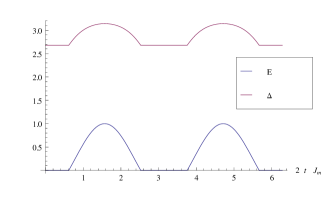
Figure 2: (Color Online) Variation of the Pancharatnam phase deficit $\Delta$ and concurrence $E$ with $\theta=2J_{m}t$ for $g_{1}=g_{4}=\pi/2$. The blue line indicates the concurrence which is always nonzero and the magenta line indicates the value of Pancharatnam phase deficit.

As evident from this equation and also illustrated in Fig. 2, nonzero Pancharatnam phase deficit is a clear signature of macroscopic entanglement in this system.

7 Conclusions

In quantum information, detection of entanglement in bipartite and multipartite states is very important. We have shown that for pure states a nonzero Pancharatnam phase deficit can detect entanglement. It happens to be a sufficient condition for entanglement and we use this to get an insight of entanglement in macroscopic superpositions of quantum states. All the entangled systems may not show the phase deficit nonzero but if it holds a nonzero value, macroscopic entanglement is witnessed. This can be a very useful method to detect entanglement in macroscopic quantum systems. We have illustrated our method to detect entanglement for macroscopic superposition of coherent states and for macroscopically distant boundary spin states. For these specific cases, we have shown that the entanglement entropy and the concurrence can be expressed directly in terms of the Pancharatnam phase deficit. Since, the Pancharatnam phase deficit can be measured in an experimental set up with the help of Mach-Zehnder interferometer, this method could easily be applied to detect entanglement of macroscopic quantum systems in the quantum interferometry.

8 Acknowledgment

NS acknowledges the research fellowship of Department of Atomic Energy.

References

• [1] \NameM. V. Berry \REVIEWProc.R. Soc.Lond A392198445.
• [2] \NameY. Aharnov, J. Anandan \REVIEWPhys. Rev. Lett.5819871593.
• [3] \NameJ. Samuel and R. Bhandari \REVIEWPhys. Rev. Lett.6019882339.
• [4] \NameS. Pancharatnam \REVIEWProc. Indian Acad. Sci. A441956247.
• [5] \NameB. Simon \REVIEWPhys. Rev. Lett.5119832167.
• [6] \NameD. M. Tong, E. Sjöqvist, L.C. Kwek, C.H. Oh, M. Ericsson \REVIEWPhys. Rev. A682003022106.
• [7] \NameX. X. Yi, L. C. Wong, T.Y. Jheng \REVIEWPhys. Rev. Lett.92200415.
• [8] \NameK. P. Marzlin, S. D. Bartlett, and B. C. Sanders \REVIEWPhys. Rev. A.672003022316.
• [9] \NameA. K. Pati \REVIEWPhys. Rev. A5219952576
• [10] \NameJ. A. Jones, V. Vedral, A. Ekert, and G. Castagnoli \REVIEWNature (London)4031999869
• [11] \NameA. Ekert, M. Ericsson, P. Hayden, H. Inamori, J.A. Jones, D. K. L. Oi, V. Vedral \REVIEWJournal of Modern Optics4720002501
• [12] \NameE. Sjöqvist and M. Hedström \REVIEWPhys. Rev. A5619973417
• [13] \NameS. R. Jain and A. K. Pati \REVIEWPhys. Rev. Lett.801998650
• [14] \NameA. K. Pati \REVIEWPhys. Rev. A601999121
• [15] \NameJ. Pachos, P. Zanardi, R. Rasetti \REVIEWPhys. Rev. A612000010305.
• [16] \NameJ. Pachos, P. Zanardi \REVIEWInt. Journal of Mod Phys. B1520011257.
• [17] \NameA. Carollo, I. F. Guridi, M. F. Santos, V. Vedral \REVIEWPhys. Rev. Lett.902003160402.
• [18] \NameE. Sjöqvist, A. K. Pati, A. Ekert, J. S. Ananadan, M. Ericsson, D. K. L. Oi, V. Vedral \REVIEWPhys. Rev. Lett.8520002845.
• [19] \NameN. J. Cerf, and C. Adami \REVIEWPhys. Rev. Lett.7919975194.
• [20] \NameR. Horodecki, and P. Horodecki \REVIEWPhys. Lett. A1971994147.
• [21] \NameD. Calvani, A. Cuccoli, N. I. Gidopoulos, and P. Verrucchi \REVIEWPNAS11020136748.
• [22] \NameJ. Hartley and V. Vedral \REVIEW J. Phys. A: Math. Gen.37200411259.
• [23] \NameB. Basu \REVIEWEurophys. Lett.732006833.
• [24] \NameE. Sjöqvist \REVIEWPhys. Rev. A622000022109.
• [25] \NameA. J. Leggett \REVIEWProg. Theor. Phys. Suppl.69198080.
• [26] \NameW. Dür, C. Simon, J.I. Cirac \REVIEWPhys. Rev. Lett.892002210402.
• [27] \NameA. Shimizu, T. Miyadera \REVIEWPhys. Rev. Lett.892003270403.
• [28] \NameG. Björk, P.G.L. Mana \REVIEW J. Opt. B: Quantum Semiclassical Opt.61980429.
• [29] \Name R. Rouse, S. Han, J. E. Luckens \REVIEWPhys. Rev. Lett.7519951614.
• [30] \NameJ. Clarke, A. N. Cleland, M. H. Devoret, D. Esteve, J. M. Martinis \REVIEWScience2391988992.
• [31] \NameP. Silvestrini, V. G. Palmieri, B. Ruggiero, M. Russao \REVIEWPhys. Rev. Lett.7919973046.
• [32] \NameY. Nakamura, Y. A. Pashkin, J. S. Tsai \REVIEWNature3981999786.
• [33] \NameJ. R. Friedman, M. P. Sarachik, J. Tejada, R. Ziolo \REVIEWPhys. Rev. Lett.7619963830.
• [34] \NameW. Wernsdorfer, E. B. Orozco, K. Hasselbach, A. Benoit, D. Mailly, O. Kubo, H. Nakano, B. Barbara \REVIEWPhys. Rev. Lett.7919974014.
• [35] \NameC. Monroe, D. M. Meekhof, B.E. King, D. J. A. Wineland \REVIEWScience27219961131.
• [36] \NameM. Brune, E. Hagley, J. Dreyer, X. Maitre, A. Malli, C. Wunderlich, J. M. Raimond, S. Haroche \REVIEWPhys. Rev. Lett.7719964887.
• [37] \NameY. Liu, L. F. Wei, and F. Nori \REVIEWPhys. Rev. A712005063820.
• [38] \NameA. Bayat, S. Bose, and P. Sodano \REVIEWPhys. Rev. Lett.1052010187204.
• [39] \NameI. Buluta and F. Nori \REVIEWScience32620095949.
• [40] \NameD. Calvani, A. Cuccoli, N. I. Gidopoulos, and P. Verrucchi \REVIEWInt. J. of Theoretical Physics5320143434.
• [41] \NameP. Liuzzo-Scorpo, A. Cuccoli, and P. Verrucchi \REVIEWEurophys. Lett.111201540008.
• [42] \NameF. D. Martini, F. Sciarrino, and C. Vitelli \REVIEWPhys. Rev. A1002008253601.
• [43] \NameS. Hill and W. K. Wootters \REVIEWPhys. Rev. Lett.78199726.