Structure of the Accretion Disk in the Lensed Quasar Q 2237+0305 from Multi-Epoch and Multi-Wavelength Narrow Band Photometry

Abstract

We present estimates for the size and the logarithmic slope of the disk temperature profile of the lensed quasar Q2237+0305, independent of the component velocities. These estimates are based on six epochs of multi-wavelength narrowband images from the Nordic Optical Telescope. For each pair of lensed images and each photometric band, we determine the microlensing amplitude and chromaticity using pre-existing mid-IR photometry to define the baseline for no microlensing magnification. A statistical comparison of the combined microlensing data (6 epochs $\times$ 5 narrow bands $\times$ 6 image pairs) with simulations based on microlensing magnification maps gives Bayesian estimates for the half-light radius of $R_{1/2}=8.5^{+7.5}_{-4.0}\sqrt{\langle M\rangle/0.3\,M_{\odot}}$ light-days, and $p=0.95\pm 0.33$ for the exponent of the logarithmic temperature profile $T\propto R^{-1/p}$. This size estimate is in good agreement with most recent studies. Other works based on the study of single microlensing events predict smaller sizes, but could be statistically biased by focusing on high-magnification events.

1 Introduction

The basic model for describing the inner regions of quasars is the thin disk model (Shakura & Sunyaev 1973; Novikov & Thorne 1973) which predicts the size of the accretion disk and the radial dependence of its surface temperature. Gravitational microlensing (Chang & Refsdal 1979, 1984; see also Kochanek 2004 and Wambsganss 2006) is the main tool used to estimate both parameters, either from time variability or through the wavelength dependence of the microlensing magnification. Microlensing studies (see e.g. Pooley et al. 2007; Morgan et al. 2010; Sluse et al. 2011, Blackburne et al. 2011, 2014, 2015; Mosquera $\&$ Kochanek 2011; Jiménez-Vicente et al. 2012, 2014; Hainline et al. 2013; Mosquera et al. 2013; MacLeod et al. 2015) have found that the mean sizes of quasar accretion disks are roughly a factor of 2-3 greater than the predictions of the standard thin disk model. These differences are too large to be explained by contamination from the broad emission lines and the pseudo-continuum contributions, or scattering on scales larger than the accretion disk (Dai et al. 2010, Morgan et al. 2010). Recent measurements of wavelength-dependent continuum lags in two local active galactic nuclei (AGNs) are consistent with the microlensing results (Shappee et al. 2014, Edelson et al. 2015, Fausnaugh et al. 2015).

The study of the disk temperature profile is more complicated because multi-wavelength observations are needed to detect chromatic microlensing (Anguita et al. 2008; Poindexter et al. 2008; Bate et al. 2008; Eigenbrod et al. 2008; Floyd et al. 2009; Blackburne et al. 2011, 2015; Mediavilla et al. 2011a; Mosquera et al. 2011; Muñoz et al. 2011; Motta et al. 2012, Rojas et al. 2014). In this case, it also becomes more important to separate the contributions from strong emission lines. Such a separation can be done most cleanly using narrow band photometry or spectroscopy.

Many of the studies of the source size in Q 2237+0305 are based on the fitting of its light curves with tracks extracted from simulated microlensing magnification maps (Kochanek 2004; Poindexter & Kochanek 2010b; Mosquera et al. 2013). As an alternative to light-curve fitting, we will study the size and temperature profile of Q 2237+0305 using several epochs of multi-wavelength narrowband observations. This allows us to remove the influence of the broad emission lines on the amplitude of the continuum microlensing (Mosquera et al. 2009). We will follow a procedure similar to that used in SBS 0909+532 (Mediavilla et al. 2011a) and HE 1104–1804 (Muñoz et al. 2011), but in the case of Q 2237+0305 we have significantly better statistics with six epochs (four will be considered independent) and four quasar images. This method relies on changes in the microlensing amplitude and chromaticity but not on its dependence with time and hence no velocity estimates are necessary. However, a baseline for the intrinsic flux ratios in the absence of microlensing is needed, and we will define these by the mid-IR flux ratios from Minezaki et al. (2009, see also Agol et al. 2000). In Section 2 we describe the observations and data. Section 3 is devoted to the statistical analysis and in Section 4 we discuss the results.

2 Observations and Data Analysis

Q 2237+0305 (Huchra et al. 1985) was observed with the 2.56 m Nordic Optical Telescope (NOT) located at the Roque de los Muchachos Observatory, La Palma (Spain). We used the 2048$\times$2048 ALSFOC detector, with a spatial scale of 0.188 arcsec/pixel. We obtained a total of five epochs in 2006 and 2007 which we combine with an earlier epoch from Mosquera et al. (2009) taken in 2003. A set of seven narrow filters plus the wide Bessel I filter were used, covering the wavelength range 3510-8130 Å. Table 1 provides a log of our observations. For the first epoch, a V-band image was also taken. In the second epoch, the wavelength coverage was poorer, because we were unable to observe with all the filters due to bad weather conditions.

The data were reduced using standard IRAF procedures, and pont-spread function (PSF) photometry fitting was used to derive the difference in magnitude as a function of wavelength between the four images. As in Mosquera et al. (2009), the galaxy bulge was modeled with a de Vaucouleurs profile, and the quasar images as point sources. This model was convolved with PSFs derived from stars observed in each of the frames, and fit to the image using $\chi^{2}$ statistics following McLeod et al. (1998) and Lehár et al. (2000). Even in the bluest filters, the fits were excellent due to the good seeing conditions for most of the epochs (0$\farcs$6 in I-band). Among the narrower filters that we used, only two were affected by the broad emission lines of the quasar. The Strömgren-u filter contains roughly 40% of the Ly$\alpha$ emission line, based on the SDSS quasar composite spectrum from Vanden Berk et al. (2001). And at $\lambda=4110$ Å, the wavelength range covered by the Strömgren-v filter coincides with the position and width of the CIV emission line (for more details see Mosquera et al., 2009).

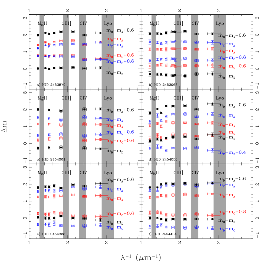
Figure 1: Magnitude differences as a function of the inverse of the observed wavelength for Q 2237+0305 during the six epochs of observation. Image A showed chromaticity on epoch HJD 2452879 (a), as previously analyzed by Mosquera et al. (2009). Here we find that image A also shows evidence of chromaticity on HJD 2454056 (d) and HJD 2454404 (f), as does image B on HJD 2454056 (d). The shaded regions correspond to the wavelength location and full width of the most prominent quasar broad emission lines. The horizontal error bars indicate the FWHM of the filters.

Figure 1 shows the results for the six nights and Table 1 reports the photometry for the new data. A clear wavelength dependence of the flux ratios $(m_{i}-m_{A})_{i=B,C,D}$ relative to image $A$ is observed for the epochs HJD 2454056 (Fig. 1d) and HJD 2454404 (Fig. 1f). Chromatic effects are also observed relative to image $B$ $(m_{i}-m_{B})_{i=A,C,D}$ on the first of these two dates. Since extinction effects would be common to all the epochs (e.g. Falco et al. 1999 or Muñoz et al. 2004) and the time delays are negligible, this dependence can only be explained by chromatic microlensing of images $A$ and $B$ (for more details see Mosquera et al., 2009). Since image $C$ seems little affected by chromatic microlensing on any of those nights, the difference $(m_{C}-m_{A})^{I}-(m_{C}-m_{A})^{b}$ allows us to determine the chromaticity in image $A$, with values of $m^{b}_{A}-m^{I}_{A}=-0.43\pm 0.16$ and $m^{b}_{A}-m^{I}_{A}=-0.33\pm 0.16$ for HJD 2454056 and HJD 2454404 respectively. In a similar way, the chromaticity for image $B$ is $m^{b}_{B}-m^{I}_{B}=-0.25\pm 0.16$ for HJD 2454056. The $I$ and $b$ filters were chosen to perform these calculations since they are the reddest and bluest filters that are not affected by the broad emission lines. The other epochs do not show any significant dependence on wavelength. In particular the magnitude difference as a function of wavelength for the epoch HJD 2454001 (Fig. 1c) is flat given our errors of order $\sim 0.1$ mag. This suggests a smaller differential extinction than the estimates of Agol et al. (2000), although we cannot rule out fortuitous cancellations of color variations due to extinction by chromatic microlensing effects. Finding chromatic microlensing during this period of observations is not a surprise, since the Optical Gravitational Lensing Experiment (OGLE) V-band continuum data (Woźniak et al., 2000) shows significant brightness variations in the three independent magnitude differences at this time. This implies that microlensing is strongly affecting the quasar images, making chromatic microlensing effects more likely.

3 Results

The statistical procedure used to estimate the size of the accretion disk and the strength of the chromaticity is a variant of that described in Mediavilla et al. (2011a), Muñoz et al. (2011) and Jiménez-Vicente et al. (2012). The main difference is that the observed magnitudes for the four quasar images in the five different bands are used simultaneously to calculate the probability distributions.

The magnification maps were calculated using the Inverse Polygon Mapping algorithm (Mediavilla et al. 2006, Mediavilla et al. 2011a). We have used canonical values for $\kappa$ and $\gamma$ for the four images from Schmidt et al. (1998) and put all the mass into equal mass stars. The models used by Poindexter $\&$ Kochanek (2010a) are very similar but with a mass spectrum for the stars. The 2000$\times$2000 pixels maps have a pixel size of 0.5 light-days for a mean stellar mass of $\langle M\rangle=1M_{\sun}$ and all linear sizes can be scaled with $(\langle M\rangle/M_{\sun})^{1/2}$. We considered three surface brightness profiles. In all three models, the scaling of the source size with wavelength is described by a power-law, $r_{s}(\lambda_{2})=(\lambda_{2}/\lambda_{1})^{p}r_{s}(\lambda_{1})$ where $\lambda_{i}$ is the rest wavelength corresponding to each filter. The first model we consider is a simple Gaussian, $I(R)\propto\exp(-R^{2}/2r_{s}^{2})$. The second model, $I(R)\propto\left(\exp\left[(R/r_{s})^{3/4}\right]-1\right)^{-1}$ becomes the standard thin disk model when $p=4/3$. The third model, $I(R)\propto\left(\exp\left[(R/r_{s})^{1/p}\right]-1\right)^{-1}$ also becomes the standard thin disk model when $p=4/3$. The third model corresponds to a thermally emitting disk with a temperature profile $T\propto R^{-1/p}$ and is well-defined only for $p>1/2$ since we are not including an inner edge. The second model is a hybrid, but by holding the exponent in the blackbody function fixed and only varying the scale length, the brightness profile is well defined for all $p$. We will refer to the three models as the Gaussian, hybrid and thin disk models. The length scales $r_{s}$ will depend on the profile and $p$, however, we expect the estimates of the half-light radii for the different profiles to agree based on the results of Mortonson et al. (2005). We use the bluest observed wavelength, $\lambda_{1}^{obs}=4670\,\rm\AA$ as the reference wavelength, corresponding to $\lambda_{1}=1736$ Å in the rest frame. When no reference is made to a specific wavelength the size is for this reference wavelength, $r_{s}\equiv r_{s}(1736\,\rm\AA)$.

The observed magnitude of image $I=(A,B,C,D)$ is

$$m_{I}^{obs}(t_{j},i)=m_{0}(t_{j},i)+\mu_{I}+\delta\mu_{I}(t_{j},i)$$ (1)

where $m_{0}(t_{j},i)$ is the intrinsic magnitude of the source at time $t_{j}$ in filter $i$, $\mu_{I}$ is the macro magnification (in mag) of image $I$ and $\delta\mu_{l}(t,i)$ is the time varying microlensing magnification (in mag) of image $I$ in filter $i$. Since we have no direct information on the intrinsic variability of the source or the absolute magnifications, we ultimately want to work in terms of magnitude differences between images. We assume that the mid-IR flux ratios from Minezaki et al. (2009) (cf. their Table 4) correctly estimate the intrinsic flux ratios $\mu_{IJ}^{ir}$, which means that they define all the values of $\mu_{IJ}^{ir}=\mu_{I}-\mu_{J}$. Following Kochanek (2004), we eliminate the intrinsic magnitude of the source $m_{0}(t_{j},i)$ by starting from the fit to the four individual images at a single epoch and wavelength

$$\chi^{2}(t_{j},i)=\sum_{I}\sigma_{I}(t_{j},i)^{-2}\left[m_{I}^{obs}(t_{j},i)-m_{0}(t_{j},i)-\mu_{I}-\delta\mu_{I}(t_{j},i)\right]^{2}$$ (2)

and optimizing for the best source model $m_{0}(t_{j},i)$. If we then substitute this best fit source model into $\chi^{2}(t_{j},i)$, we are left with a sum over the six possible pairs between the four images

$$\chi^{2}(t_{j},i)=\sum_{I}\sum_{J>I}\sigma_{IJ}(t_{j},i)^{-2}\left[\Delta m_{I}(t_{j},i)-\Delta m_{J}(t_{j},i)\right]^{2}$$ (3)

where

$$\Delta m_{I}(t_{j},i)=m_{I}^{obs}(t_{j},i)-\mu_{I}-\delta\mu_{I}(t_{j},i)$$ (4)

and the errors $\sigma_{IJ}(t_{j},i)$ are defined in the equation 7 of Kochanek (2004) but reduce to $\sigma_{IJ}(t_{j},i)=2\,\sigma(t_{j},i)$ if $\sigma_{I}=\sigma_{J}(\equiv\sigma)$ as we will assume here. This expression only depends on $\mu_{I}-\mu_{J}$, whose values are supplied by the mid-IR flux ratios. Thus, the full $\chi_{j}^{2}$ for a given epoch $t_{j}$ becomes the sum of Equation 3 over the filters,

$$\chi_{j}^{2}=\sum_{i}\chi^{2}(t_{j},i)$$ (5)

which can be evaluated for any microlensing trial defining the values of $\delta\mu_{I}(t_{j},i)$.

For a given pair of parameters $(r_{s},p)$, the magnification maps for the four images $A,B,C,D$ are convolved to the size $r_{s}(\lambda/\lambda_{0})^{p}$ appropriate for each wavelength and the $\chi_{j}^{2}$ are calculated for N=$10^{8}$ randomly selected locations in each of the four magnification maps. The probability density function $P_{j}(r_{s},p)$ for each epoch is computed as the sum

$$P_{j}(r_{s},p)\propto\sum_{i=1}^{N}{{{e^{-{1\over 2}\chi_{j}^{2}}}}}$$ (6)

over a 2D grid of values for $r_{s}$ and $p$. We have used a logarithmic grid in $r_{s}$ such that $\ln(r_{s}^{i}/\mbox{light-days})=0.3\times i$ for $i=0,\cdots,17$ and a linear grid in $p$ with $p^{j}=0.25\times j$ for $j=0,\cdots,9$. This way, $r_{s}$ spans from roughly 1 to 165 light-days and $p$ runs from 0 to 2.25. For the thin disk model, which is only defined for $p>1/2$, we ran extra cases at $p=0.55$ and $0.68$ and then follow the remainder of the sequence.

We have data for six different epochs between August 2003 and October 2007. Some of the epochs are very close on time and we have combined them into a single epoch because they cannot be considered independent. Epoch HJD 2453968 (Aug 21st 2006) is combined with HJD 2454001 (Sep 23rd 2006) and epoch HJD 2454388 (Oct 15th 2007) is combined with HJD 2454404 (Oct 31st 2007). The dispersion around the mean for all values of the combined epochs is 0.08 mags, which is the same as the measurement error we adopted for the merit function above.

The joint probability distribution ${\cal P}(r_{s},p)$ for the four independent epochs is obtained by the product of the probabilities for each of the epochs

$${\cal P}(r_{s},p)=\prod_{j}P_{j}(r_{s},p)$$ (7)

The resulting joint probability distributions of the three surface brightness profiles are shown in Figure 2 and are compared to previous size estimates for Q 2237+0305 in Figure 3. The maximum likelihood estimate corresponds to $r_{s}=(15.6^{+5.5}_{-7.9},5.3^{+1.9}_{-2.4},27^{+22}_{-19})$ $\sqrt{\langle M\rangle/0.3M_{\odot}}$ light-days and $p=(0.50^{+0.15}_{-0.27},1.0^{+0.25}_{-0.50},0.85^{+0.25}_{-0.25})$ for the Gaussian, hybrid and thin disk models respectively. Using a logarithmic (linear) prior for $r_{s}$ ($p$), we obtain Bayesian estimates for the expected values of $r_{s}=(7.0^{+10.0}_{-4.1},3.7_{-1.8}^{+3.5},7.9_{-5.3}^{+16.6})\sqrt{\langle M\rangle/0.3M_{\odot}}$ light-days and $p=(0.66\pm 0.32,1.04\pm 0.29,0.95\pm 0.33)$. As a test we also computed the joint probability distribution without merging the closely separated epochs and obtained very similar results.

4 Discussion and Conclusions

At $\lambda_{1}=1736\$Å, the half-light radius estimates for the three (Gaussian, hybrid, and thin disk) models of $R_{1/2}=(8.3^{+11.8}_{-4.8},9.0^{+8.4}_{-4.4},8.5_{-4.0}^{+7.5})\sqrt{\langle M\rangle/0.3M_{\odot}}$ light-days are remarkably similar (see Figure 2), consistent with the prediction from Mortonson et al. (2005) that estimates of the half-light radius should be insensitive to the particular surface brightness profile shape. Our $R_{1/2}$ estimations are also in agreement with previous estimates by Poindexter & Kochanek (2010b; $R_{1/2}=5.4\pm 3.2$ light-days), Sluse et al. (2011; $R_{1/2}=3.4^{+6.4}_{-2.4}$ light-days) and Mosquera et al. (2013; $R_{1/2}=9.9^{+5.1}_{-3.3}$ light-days), as shown in Figure 3. The latter two results are also scaled to $\langle M\rangle=0.3M_{\odot}$. The Poindexter & Kochanek (2010b) result marginalizes over the uncertainties in $\langle M\rangle$, finding $\langle M\rangle=0.52M_{\odot}$ ($0.12M_{\odot}<M<1.94M_{\odot}$). Poindexter & Kochanek (2010ab), Mosquera et al. (2013) and Sluse et al. (2011) set the scales by adopting priors on the effective source velocity rather than choosing a fixed mean mass $\langle M\rangle$. That our results agree demonstrates that these priors are reasonable.

Analyses of individual high magnification events tend to measure smaller sizes. For example Anguita et al. (2008) find $R_{1/2}=1.0^{+0.2}_{-0.5}$ light-days and Eigenbrod et al. (2008) find $R_{1/2}=3.0\pm 2.0$ light-days. However, studies of high magnification events are likely biased toward small quasar size estimates because it is easier to obtain high magnifications with small sources (e.g. Kochanek 2004; Eigenbrod et al. 2008; Blackburne et al. 2011). It is also interesting to note that without considering any velocity prior (i.e. adopting a uniform prior), the size determinations of Eigenbrod et al. (2008) and Anguita et al. (2008) increase by a factor $\sim 4$ (see Sluse et al. 2011) but would then require cosmologically unrealistic peculiar velocities for the lens/source.

In any case, most of the results derived from the optical may be reconciled near a value of $\sim(7\pm 4)\sqrt{\langle M\rangle/0.3M_{\odot}}$ light-days. This value is large compared to the predictions of the thin disk model based on the flux ($\sim 1$ light-day, Mosquera $\&$ Kochanek 2011). It is in agreement with the results from other lenses, where the Morgan et al. (2010) black hole-mass-size correlation predicts a size of $\sim 5$ light-days for an estimated black hole mass of $1.2\times 10^{9}M_{\odot}$ (Assef et al. 2011). This size discrepancy is now also seen in the recent size estimates for two local AGN using measurements of continuum lags (Shappee et al. 2014, Edelson et al. 2015, Fausnaugh et al. 2015). The size problem is clearly not unique to the microlensing method.

The hybrid and thin disk models both find $p=1.0\pm 0.3$ for the slope of the dependence of the disk size on wavelength, while the Gaussian model favors a steeper (in temperature) slope of $p=0.7\pm 0.3$. The three estimates are mutually compatible and smaller than the prediction of the standard thin disk model ($p=4/3$). The differences for the (presumably) more physical hybrid or thin disk models are small enough to represent only a modest inconsistency. Experiments with broader wavelength ranges are needed to provide better estimates of the temperatures exponent.

Acknowledgments: This research was supported by the Spanish Ministerio de Educación y Ciencia with the grants AYA2010-21741-C03-01/02, AYA2011-24728, AYA2013-47744-C3-1/3-P and AYA2014-53506-P. JAM is also supported by the Generalitat Valenciana with the grant PROMETEO/2014/60. JJV is also supported by the Junta de Andalucía through the FQM-108 project. AMM is supported by NSF grant AST-1211146.

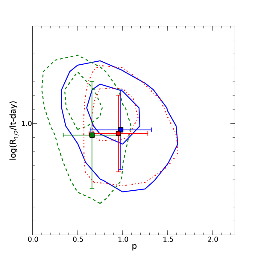
Figure 2: Joint probability density function ${\cal P}(r_{s},p)$ in terms of the half-light radius $R_{1/2}$, at rest $\lambda_{1}=1736$ Å, and the logarithmic slope $p$ ($r_{s}\propto\lambda^{p}$). The contours for each model correspond to the 1-$\sigma$ and 2-$\sigma$ levels for one parameter. The Gaussian, hybrid and thin disk models are shown by the green (dashed), blue (solid) and dotted (red) colors (lines). The filled squares are the Bayesian estimates for the expected values of $R_{1/2}$ and $p$.

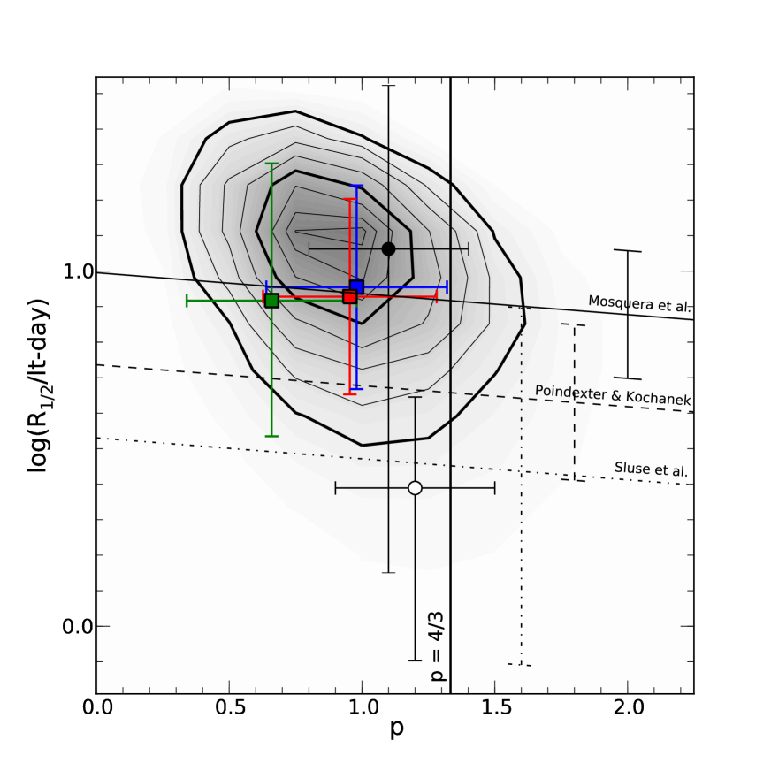
Figure 3: Joint probability density function ${\cal P}(r_{s},p)$ in terms of the half-light radius $R_{1/2}$, at rest $\lambda_{1}=1736$ Å, and the logarithmic slope $p$ ($r_{s}\propto\lambda^{p}$) for the hybrid model. The separation between consecutive contours corresponds to 0.25 $\sigma$, the 1-$\sigma$ and 2-$\sigma$ for one parameter contours are heavier. The blue filled square is our Bayesian estimate for the expected value of $R_{1/2}$ and $p$ for the hybrid model (the values for the Gaussian and thin disk models are also plotted as green and red filled squares respectively for comparison). The open (filled) circle corresponds to the measurement by Eigenbrod et al (2008) with (without) a velocity prior. Straight lines correspond to the measurements by Poindexter & Kochanek 2010b (dashed line), Sluse et al. 2011 (dotted-dashed line) and Mosquera et al. 2013 (continuous line), that have no estimate on $p$; the associated error bars correspond to their $\pm 1\sigma$ uncertainties. The size comparisons have been made setting the mean mass of the stars to $\langle M\rangle=0.3\,M_{\odot}$.

Table 1: Q 2237+0305 PHOTOMETRY

Filter	$m_{B}-m_{A}$	$m_{C}-m_{A}$	$m_{D}-m_{A}$	Observation date
Str-u ($\lambda=3510$ Å)	1.18$\pm$0.07	1.56$\pm$0.11	1.47$\pm$0.06	Aug 21 2006
Str-v ($\lambda=4110$ Å)	1.15$\pm$0.06	1.58$\pm$0.08	1.46$\pm$0.06	Aug 21 2006
Str-b ($\lambda=4670$ Å)	1.19$\pm$0.06	1.59$\pm$0.07	1.61$\pm$0.06	Aug 21 2006
V-band ($\lambda=5300$ Å)	1.19$\pm$0.04	1.64$\pm$0.06	1.56$\pm$0.06	Aug 21 2006
Str-y ($\lambda=5470$ Å)	1.19$\pm$0.03	1.59$\pm$0.05	1.59$\pm$0.04	Aug 21 2006
Iac#28 ($\lambda=6062$ Å)	1.14$\pm$0.10	1.50$\pm$0.10	1.51$\pm$0.10	Aug 21 2006
H$\alpha$ ($\lambda=6567$ Å)	1.15$\pm$0.06	1.51$\pm$0.08	1.47$\pm$0.03	Aug 21 2006
Iac#29 ($\lambda=7015$ Å)	1.16$\pm$0.06	1.54$\pm$0.06	1.48$\pm$0.06	Aug 21 2006
I-band ($\lambda=8130$ Å)	1.16$\pm$0.08	1.59$\pm$0.15	1.48$\pm$0.06	Aug 21 2006
Str-u ($\lambda=3510$ Å)	1.13$\pm$0.08	1.49$\pm$0.05	1.44$\pm$0.07	Sep 23 2006
Str-v ($\lambda=4110$ Å)	1.13$\pm$0.10	1.55$\pm$0.10	1.41$\pm$0.10	Sep 23 2006
Str-y ($\lambda=5470$ Å)	1.10$\pm$0.10	1.39$\pm$0.10	1.34$\pm$0.10	Sep 23 2006
H$\alpha$ ($\lambda=6567$ Å)	1.14$\pm$0.05	1.47$\pm$0.08	1.38$\pm$0.06	Sep 23 2006
I-band ($\lambda=8130$ Å)	1.15$\pm$0.06	1.53$\pm$0.09	1.41$\pm$0.06	Sep 23 2006
Str-u ($\lambda=3510$ Å)	1.22$\pm$0.09	1.74$\pm$0.08	1.74$\pm$0.10	Nov 17 2006
Str-v ($\lambda=4110$ Å)	1.14$\pm$0.02	1.57$\pm$0.03	1.41$\pm$0.03	Nov 17 2006
Str-b ($\lambda=4670$ Å)	1.22$\pm$0.05	1.74$\pm$0.09	1.63$\pm$0.05	Nov 17 2006
Str-y ($\lambda=5470$ Å)	1.22$\pm$0.08	1.73$\pm$0.11	1.60$\pm$0.06	Nov 17 2006
Iac#28 ($\lambda=6062$ Å)	1.30$\pm$0.03	1.59$\pm$0.07	1.62$\pm$0.04	Nov 17 2006
H$\alpha$ ($\lambda=6567$ Å)	1.02$\pm$0.08	1.38$\pm$0.07	1.22$\pm$0.04	Nov 17 2006
Iac#29 ($\lambda=7015$ Å)	1.17$\pm$0.07	1.64$\pm$0.12	1.43$\pm$0.05	Nov 17 2006
I-band ($\lambda=8130$ Å)	1.05$\pm$0.08	1.31$\pm$0.13	1.19$\pm$0.08	Nov 17 2006
Str-u ($\lambda=3510$ Å)	1.33$\pm$0.10	1.84$\pm$0.09	1.44$\pm$0.09	Oct 15 2007
Str-v ($\lambda=4110$ Å)	1.28$\pm$0.06	1.74$\pm$0.10	1.29$\pm$0.06	Oct 15 2007
Str-b ($\lambda=4670$ Å)	1.37$\pm$0.05	1.83$\pm$0.05	1.37$\pm$0.04	Oct 15 2007
Str-y ($\lambda=5470$ Å)	1.31$\pm$0.04	1.63$\pm$0.10	1.18$\pm$0.06	Oct 15 2007
Iac#28 ($\lambda=6062$ Å)	1.28$\pm$0.10	1.60$\pm$0.09	1.29$\pm$0.10	Oct 15 2007
H$\alpha$ ($\lambda=6567$ Å)	1.24$\pm$0.06	1.63$\pm$0.10	1.25$\pm$0.06	Oct 15 2007
Iac#29 ($\lambda=7015$ Å)	1.25$\pm$0.08	1.63$\pm$0.08	1.26$\pm$0.06	Oct 15 2007
I-band ($\lambda=8130$ Å)	1.25$\pm$0.06	1.58$\pm$0.06	1.21$\pm$0.06	Oct 15 2007
Str-u ($\lambda=3510$ Å)	1.43$\pm$0.03	2.06$\pm$0.09	1.48$\pm$0.04	Oct 31 2007
Str-v ($\lambda=4110$ Å)	1.32$\pm$0.08	1.89$\pm$0.10	1.37$\pm$0.09	Oct 31 2007
Str-b ($\lambda=4670$ Å)	1.39$\pm$0.09	2.02$\pm$0.10	1.46$\pm$0.07	Oct 31 2007
Str-y ($\lambda=5470$ Å)	1.37$\pm$0.08	1.98$\pm$0.10	1.43$\pm$0.06	Oct 31 2007
Iac#28 ($\lambda=6062$ Å)	1.33$\pm$0.09	1.97$\pm$0.11	1.45$\pm$0.08	Oct 31 2007
H$\alpha$ ($\lambda=6567$ Å)	1.34$\pm$0.06	1.82$\pm$0.10	1.40$\pm$0.08	Oct 31 2007
Iac#29 ($\lambda=7015$ Å)	1.24$\pm$0.06	1.67$\pm$0.10	1.21$\pm$0.02	Oct 31 2007
I-band ($\lambda=8130$ Å)	1.22$\pm$0.08	1.69$\pm$0.12	1.22$\pm$0.08	Oct 31 2007

References

- Agol et al. (2000) Agol, E., Jones, B., & Blaes, O. 2000, ApJ, 545, 657
- Anguita et al. (2008) Anguita, T., Schmidt, R. W., Turner, E. L., Wambsganss, J., Webster, R. L., Loomis, K. A., Long, D., McMillan, R. 2008, A&A, 480, 327
- Assef et al. (2011) Assef, R. J., Denney, K. D., Kochanek, C. S., et al. 2011, ApJ, 742, 93
- Bate et al. (2008) Bate, N. F., Floyd, D. J. E., Webster, R. L., Wyithe, J. S. B. 2008, MNRAS, 391, 1955
- Blackburne et al. (2011) Blackburne, J. A., Pooley, D., Rappaport, S., Schechter, P. L. 2011, ApJ, 729, 34
- Blackburne et al. (2014) Blackburne, J. A., Kochanek, C. S., Chen, B., Dai, X., Chartas, G. 2014, ApJ, 789, 125
- Blackburne et al. (2015) Blackburne, J. A., Kochanek, C. S., Chen, B., Dai, X., Chartas, G. 2015, ApJ, 798, 95
- Chang & Refsdal (1979) Chang, K., & Refsdal, S. 1979, Nature, 282, 561
- Chang & Refsdal (1984) Chang, K., & Refsdal, S. 1984, A&A, 132, 168
- Dai et al. (2010) Dai, X., Kochanek, C. S., Chartas, G., Kozlowski, S., Morgan, C. W., Garmire, G., Agol, E. 2010, ApJ, 709, 278
- Edelson et al. (2015) Edelson, R., Gelbord, J. M., Horne, K., et al. 2015, ApJ, 806, 129
- Eigenbrod et al. (2008) Eigenbrod, A., Courbin, F., Meylan, G., Agol, E., Anguita, T., Schmidt, R. W., Wambsganss, J. 2008, A&A, 490, 933
- Falco et al. (1999) Falco, E. E., Impey, C. D., Kochanek, C. S., et al. 1999, ApJ, 523, 617
- Fausnaugh et al. (2015) Fausnaugh et al. 2015, in preparation
- Floyd et al. (2009) Floyd, D. J. E., Bate, N. F., Webster, R. L. 2009, MNRAS, 398, 233
- Hainline et al. (2013) Hainline, L. J., Morgan, C. W., MacLeod, C. L., et al. 2013, ApJ, 774, 69
- Huchra et al. (1985) Huchra, J., Gorenstein, M., Kent, S., Shapiro, I., Smith, G., Horine, E., Perley, R. 1985, AJ, 90, 691
- Jiménez-Vicente et al. (2014) Jiménez-Vicente, J., Mediavilla, E., Kochanek, C. S., et al. 2014, ApJ, 783, 47
- Jiménez-Vicente et al. (2012) Jiménez-Vicente, J., Mediavilla, E., Muñoz, J. A., Kochanek, C. S. 2012, ApJ, 751:106
- Kochanek (2004) Kochanek, C. S. 2004, ApJ, 605, 58
- Lehár et al. (2000) Lehár, J.; Falco, E. E.; Kochanek, C. S., et al. 2000, ApJ, 536, 584
- MacLeod et al. (2015) MacLeod, C. L., Morgan, C. W., Mosquera, A. M., et al. 2015, ApJ, 806, 258
- McLeod et al. (1998) McLeod, B. A., Bernstein, G. M., Rieke, M. J., Weedman, D. W. 1998, AJ, 115, 1377
- Mediavilla et al. (2006) Mediavilla, E., Muñoz, J. A., Lopez, P., et al. 2006, ApJ, 653, 942
- Mediavilla et al. (2011a) Mediavilla, E., Muñoz, J. A., Kochanek, et al. 2011a, ApJ, 730, 16
- Mediavilla et al. (2011b) Mediavilla, E., Mediavilla, T., Muñoz, J. A., et al. 2011b, ApJ, 741, 42
- Minezaki et al. (2009) Minezaki, T., Chiba, M. Kashikawa, N., Inoue, K. T. & Kataza, H. 2009, ApJ, 697, 610
- Morgan et al. (2010) Morgan, C. W., Kochanek, C. S., Morgan, N. D., Falco, E. E. 2010, ApJ, 712, 1129
- Mortonson et al. (2005) Mortonson, M. J., Schechter, Paul L., Wambsganss, J. 2005, ApJ, 628, 594
- Mosquera et al. (2009) Mosquera, A. M., Muñoz, J. A., Mediavilla, E. 2009, ApJ, 691, 1292
- Mosquera et al. (2011a) Mosquera, A. M., Muñoz, J. A., Mediavilla, E., Kochanek C. S. 2011, ApJ, 728, 145
- Mosquera Kochanek (2011b) Mosquera, A. M., Kochanek, C. S. 2011, ApJ, 738, 96
- Mosquera et al. (2013) Mosquera, A. M., Kochanek, C. S., Chen, B., et al. 2013, ApJ, 769, 53
- Motta et al. (2012) Motta, V., Mediavilla, E., Falco, E., Muñoz, J. A. 2012, ApJ, 755, 82
- Muñoz et al. (2004) Muñoz, J. A., Falco, E. E., Kochanek, C. S., McLeod, B. A., & Mediavilla, E. 2004, ApJ, 605, 614
- Muñoz et al. (2011) Muñoz, J. A., Mediavilla, E., Kochanek, C. S., Falco, E. E., Mosquera, A. M. 2011, ApJ, 742, 67
- Novikov & Thorne (1973) Novikov, I. D., & Thorne, K. S. 1973, Black Holes (Les Astres Occlus), 343
- Poindexter et al. (2008) Poindexter, S., Morgan, N., Kochanek, C. S. 2008, ApJ, 673, 34
- Poindexter Kochanek (2010a) Poindexter, S., Kochanek, C. S. 2010a, ApJ, 712, 658
- Poindexter Kochanek (2010b) Poindexter, S., Kochanek, C. S. 2010b, ApJ, 712, 668
- Pooley et al. (2007) Pooley, D., Blackburne, J. A., Rappaport, S., Schechter, P. L. 2007, ApJ, 661, 19
- Rojas et al. (2014) Rojas, K., Motta, V., Mediavilla, E., et al. 2014, ApJ, 797, 61
- Schmidt et al. (1998) Schmidt, R., Webster, R. L., Lewis, G. F. 1998, MNRAS, 295,488
- Shakura Sunyaev (1973) Shakura, N. I., Sunyaev, R. A. 1973, A&A, 24, 337
- Shappee et al. (2014) Shappee, B. J., Prieto, J. L., Grupe, D., et al. 2014, ApJ, 788, 48
- Sluse et al. (2011) Sluse, D., Schmidt, R., Courbin, F., Hutsemékers, D., Meylan, G., Eigenbrod, A., Anguita, T., Agol, E., Wambsganss, J. 2011, A&A, 528, 100
- Vanden Berk et al. (2001) Vanden Berk, D. E., Richards, G. T., Bauer, A., et al. 2001, AJ, 122, 549
- Wambsganss (2006) Wambsganss, J. 2006, in Saas-Fee Advanced Course 33, Gravitational Lensing: Strong, Weak and Micro, ed. G. Meylan, P. Jetzer, P. North (Berlin: Springer), 453
- Woźniak et al. (2000) Woźniak, P. R., Alard, C., Udalski, A., et al. 2000, ApJ, 529, 88