Quantum gate learning in qubit networks: Toffoli gate without time dependent control

Abstract

We put forward a strategy to encode a quantum operation into the unmodulated dynamics of a quantum network without the need of external control pulses, measurements or active feedback. Our optimization scheme, inspired by supervised machine learning, consists in engineering the pairwise couplings between the network qubits so that the target quantum operation is encoded in the natural reduced dynamics of a network section. The efficacy of the proposed scheme is demonstrated by the finding of uncontrolled four-qubit networks that implement either the Toffoli gate, the Fredkin gate, or remote logic operations. The proposed Toffoli gate is stable against imperfections, has a high-fidelity for fault tolerant quantum computation, and is fast, being based on the non-equilibrium dynamics.

Introduction

Computational devices based on the laws of quantum mechanics hold promise to speed up many algorithms known to be hard for classical computers Nielsen and Chuang (2000). The implementation of a full scale computation with existing technology requires an outstanding ability to maintain quantum coherence (i.e. isolation from the environment) without compromising the ability to control the interactions among the qubits in a scalable way. Among the most successful paradigms of quantum computation, there is the “circuit model”, where the algorithm is decomposed into an universal set of single- and two-qubit gates Barenco et al. (1995), and, to some extent, the so-called adiabatic quantum computation (AQC) Aharonov et al. (2008) where the output of the algorithm is encoded in the ground state of an interacting many-qubit Hamiltonian. A different approach Benjamin and Bose (2003) is based on the use of always-on interactions, naturally occurring between physical qubits, to accomplish the computation. Compared to the circuit model, this scheme has the advantage of requiring minimal external control and avoiding the continuous switch off and on of the interactions between all but two qubits; while compared to AQC it has the advantage of being faster, being based on the non-equilibrium evolution of the system. Quantum computation with always-on interactions is accomplished by combining the natural couplings with a moderate external control, e.g. with a smooth shifting of Zeeman energies Benjamin and Bose (2004), via feedforward techniques Satoh et al. (2015), using measurement based computation Li et al. (2011) or quantum control Burgarth et al. (2010); Müller et al. (2011). Most of these approaches are based on the assumption that the natural couplings are fixed by nature and not tunable, while local interactions can be modulated with external fields. However, the amount of external control required can be minimized if the couplings between the qubits can be statically tuned Banchi et al. (2011), e.g. during the creation of the quantum device.

The recent advances in the fabrication of superconducting quantum devices has opened up to the realization of interacting quantum networks. In a superconducting device, the qubits are built with a Josephson tunnel element, an inductance and a capacitor Devoret and Schoelkopf (2013), while local operations and measurements are performed by coupling the qubit to a resonator Wallraff et al. (2004). The interactions can be designed using lithographic techniques by jointly coupling two qubits via a capacitor Barends et al. (2013) or an inductance Chen et al. (2014), and can be modeled via an effective two-body Hamiltonian ${\sum_{\alpha}}J_{\alpha}\sigma_{\alpha}{\otimes}\sigma_{\alpha}$ Geller et al. (2014); Neeley et al. (2010), where $\sigma_{\alpha}$ are the Pauli matrices. Because of the flexibility in wiring the pairwise interactions among the qubits, it is possible to arrange them in a planar graph structure, namely a collection of vertices and links, where the vertices correspond to the qubits and the links correspond to the 2-body interactions between them. Moreover, thanks to the development of three-dimensional superconducting circuits Paik et al. (2011), it may be possible in the near future to wire also non-planar configurations, namely a general qubit network.

Motivated by the above arguments, we consider the question whether it is possible to encode a quantum algorithm into the unmodulated dynamics of a suitably large quantum network of pairwise interacting qubits. This would be extremely interesting, as it would enable quantum computation by simply “waiting”, without the need of continuously applying external control pulses or measurements. Even when sequential operations cannot be avoided, our scheme can enable the in-hardware

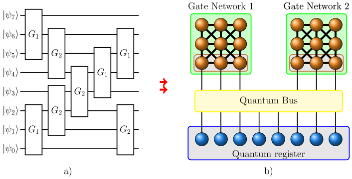
Figure 1: Schematic transposition of a quantum circuit to a trained quantum network. (a) An example 7-qubit circuit where the gates $G_{1}$ and $G_{2}$ are sequentially applied. Many important circuits can be cast into the scheme (a), such as those for quantum arithmetics Vedral et al. (1996). (b) Quantum network implementation of (a): each qubit network in the green boxes implements either $G_{1}$ or $G_{2}$ on the input/output qubits (the three qubits in the bottom row). The quantum bus sequentially transfers the state of three qubits from the register, upon which the gate $G_{1}$ or $G_{2}$ has to be applied, to the input/output qubits of the gate network. After the gate network has implemented its transformations, the state is transferred back to the original three-qubits of the register.

implementation of recurring multi-qubit operations of a quantum algorithm (see e.g. Fig.1), such as quantum arithmetic operations Vedral et al. (1996), and possibly also the quantum Fourier transform or error correcting codes Nielsen and Chuang (2000). We focus on two-body interactions, since they are the most common in physical setups, and we consider an enlarged network where auxiliary qubits enrich the quantum dynamics. The important question analyzed in this paper is the following: given a target unitary operation $U_{Q}$ on a given set of qubits $Q$, we consider an extended network $Q{\cup}A$ where $A$ is a set of auxiliary qubits (ancillae), and we ask whether it is possible to engineer the pairwise interactions in $Q{\cup}A$, modeled by the time-independent Hamiltonian $H_{QA}$, such that $e^{itH_{QA}}{=}U_{Q}{\otimes}V_{A}$ after some time $t$ ($V_{A}$ may be an extra unitary operation on the auxiliary space). More generally the target operation can depend also on the ancillae initial state: if $e^{itH_{QA}}{=}\sum_{n}U^{(n)}_{Q}{\otimes}{\left|{A_{n}}\right\rangle}{\langle{A_{n}}|}$, where $\{\left|{A_{n}}\right\rangle\}$ form a basis of the ancillae Hilbert space and, e.g., $U_{Q}{=}U^{(1)}_{Q}$, then the target operation is implemented when $A$ is initialized in $\left|{A_{1}}\right\rangle$. Our method is particularly useful for implementing quantum gates which requires $k$-body interactions ($k{>}2$), such as the Toffoli or Fredkin gates Fedorov et al. (2011); Cory et al. (1998); Nielsen and Chuang (2000) where $U_{Q}{\neq}e^{itH_{Q}}$ for any 2-local $H_{Q}$, and for remote logic, namely for applying a gate to qubits which are not directly connected but are rather interacting via intermediate systems. Our approach is completely different from the simulation of $k$-local Hamiltonians with pairwise interactions discussed in the AQC literature Bravyi et al. (2008); Biamonte and Love (2008), being based on the unmodulated dynamics. Moreover, being based on unmodulated (time-independent) interactions and ancillary qubits, it is significantly different from quantum optimal control Brif et al. (2010).

Our quantum network design procedure is inspired by supervised learning in feedforward networks Bishop (2006), where the training procedure involves the optimization of the network couplings (i.e. the weights between different nodes) such that the output corresponding to some input data has a desired functional form (e.g. for data classification). Although there are many recent developments about using a quantum device to speed-up machine learning algorithms Wittek (2014); Rebentrost et al. (2014); Paparo et al. (2014); Wiebe et al. (2015); Lloyd et al. (2014) or storing data Rotondo et al. (2015), our optimization procedure is entirely classical, but specifically developed for quantum hardware design. Our scheme is completely different from other recent proposals Nagaj (2012); Bang et al. (2008); Gammelmark and Mølmer (2009) because it avoids measurements or active feedbacks and requires minimal external control.

Results

Supervised quantum network design

Supervised learning is all about function approximation: given a training set $\{(I_{1},O_{1}),(I_{2},O_{2}),\dots\}$, namely a collection of inputs $I_{k}$ and the corresponding known outputs $O_{k}$, the goal is to find a function $f$ with two desired properties: i) $O_{k}{\simeq}f(I_{k})$ for any training pair; ii) $f$ should be able to infer the unknown output of an input not contained in the training set. In classical feedforward networks, the function $f$ is approximated with a directed graph organized in layers, where the first layer is the input register and the last one encodes the output. The value $s_{k}^{(\ell)}$ of the $k$-th node in layer $\ell$ is updated via the equation $s^{(\ell)}_{k}{=}A^{\ell}\left[\sum_{j}\lambda_{kj}^{(\ell{-}1)}s^{(\ell{-}1)}_{j}\right]~{},$ where $A^{\ell}$ is an appropriate (typically non-linear) activation function and $\lambda_{kj}^{(\ell{-}1)}$ is the weight between node $k$ in layer $\ell$ and node $j$ in $\ell{-}1$. The training procedure consists in finding the optimal weights $\boldsymbol{\lambda}$ by minimizing a suitable cost function such as $\mathcal{C}{=}\sum_{k}|O_{k}{-}f(I_{k})|^{2}$.

A quantum network consists on the other hand of an undirected graph $(V,E)$ of vertices $V$ and links $E$ described by a 2-local Hamiltonian

$$\mathcal{H}=\sum_{(n,m)\in E}\sum_{\alpha,\beta}J^{\alpha\beta}_{nm}\frac{\sigma_{n}^{\alpha}\sigma_{m}^{\beta}}{4}+\sum_{n\in V}\sum_{\alpha}h^{\alpha}_{n}\frac{\sigma_{n}^{\alpha}}{2}~{},$$ (1)

where $\sigma_{n}^{\alpha}$, $\alpha{=}x,y,z$, are the Pauli matrices acting on qubit $n$ and, to simplify the notation, we call $\boldsymbol{\lambda}{=}\{J^{\alpha\beta}_{nm},h^{\alpha}_{n}\}$ the set of parameters. The vertices are composed of two disjoints sets $V{=}Q{\cup}A$ where $Q$ consists of register qubits and $A$ of auxiliary qubits. Given a separable initial state $\left|{\psi_{Q}}\right\rangle{\otimes}\left|{\psi_{A}}\right\rangle$, the time evolution according to Hamiltonian (1) generates a quantum channel Nielsen and Chuang (2000) $\mathcal{E}_{\boldsymbol{\lambda}}[\left|{\psi_{Q}}\right\rangle\langle{\psi_{Q}}|]{=}\operatorname*{Tr}_{A}[e^{-i\mathcal{H}\tilde{t}}\left|{\psi_{Q}}\right\rangle\langle{\psi_{Q}}|{\otimes}\left|{\psi_{A}}\right\rangle\langle{\psi_{A}}|e^{i\mathcal{H}\tilde{t}}]$ on subsystem $Q$ – since we are interested in a fixed operational time $\tilde{t}$ for simplicity we set $\tilde{t}{=}1$, reabsorbing $\tilde{t}$ into the definition of the definition of $\mathcal{H}$. Depending on the flexibility of the experimental apparatus in reliably initializing the auxiliary qubits, one can add $\left|{\psi_{A}}\right\rangle$ to the set $\boldsymbol{\lambda}$. Network design consists in the following procedure: given a target unitary operation $U_{Q}$ that we want to implement, the goal is to find the parameters $\boldsymbol{\lambda}$, if they exist, such that $\mathcal{E}_{\boldsymbol{\lambda}}[\rho_{Q}]{=}U_{Q}\rho_{Q}U_{Q}^{\dagger}$ for any $\rho_{Q}$. To simplify the notation we assume that the gate output is encoded in $Q$ but it is straightforward to generalize the formalism when the output sites differ from the input ones.

Motivated by the similarity with classical supervised learning, where the weights $\boldsymbol{\lambda}$ are tuned to maximize the ability of the network to reproduce a known output given the corresponding input, we create a training set $\mathcal{T}$ with a random set of initial input states. For each input $\left|{\psi}\right\rangle{\in}\mathcal{T}$ the expected known output is $U_{Q}\left|{\psi}\right\rangle$, while the output of the network evolution is $\mathcal{E}_{\boldsymbol{\lambda}}[\left|{\psi}\right\rangle\langle{\psi}|]$. The “learning” procedure involves the minimization of the difference between the output of the network and the expected output, and corresponds to the maximization of the fidelity

$$\mathcal{F} =\sum_{\left|{\psi}\right\rangle\in\mathcal{T}}\frac{\mathcal{F}_{\psi}}{|\mathcal{T}|}, \mathcal{F}_{\psi} =\langle{\psi}|U_{Q}^{\dagger}\mathcal{E}_{\boldsymbol{\lambda}}\left[\left|{\psi}\right\rangle\langle{\psi}|\right]U_{Q}\left|{\psi}\right\rangle.$$ (2)

If the average is performed over all possible states, then Eq.(2) can be substituted by the average gate fidelity $\bar{\mathcal{F}}{=}\int\mathcal{F}_{\psi}d\psi$ where the formal integration can be explicitly evaluated Banchi et al. (2011); Magesan et al. (2011); Pedersen et al. (2008) yielding

$$\bar{\mathcal{F}}=\frac{1}{D+1}+\frac{1}{D(D+1)}\sum_{ijkl}U_{ik}^{*}\mathcal{E}^{ij,kl}_{\boldsymbol{\lambda}}U_{jl}~{},$$ (3)

where $\mathcal{E}^{ij,kl}_{\boldsymbol{\lambda}}{=}\langle{q_{i}}|\mathcal{E}_{\boldsymbol{\lambda}}\big{[}|{q_{k}}\rangle\langle{q_{l}}|\big{]}|{q_{j}}\rangle$, $U_{ij}{=}\langle{q_{i}}|U_{Q}\left|{q_{j}}\right\rangle$ and $\{\left|{q_{j}}\right\rangle\}$ form the computational basis of the $D$-dimensional Hilbert space of qubits $Q$. The typical value of the fidelity for a random non-optimal evolution of the qubit network is $\bar{\mathcal{F}}{=}D^{-1}$, obtained using Haar integration techniques Collins and Śniady (2006). This value is independent on the details of the ancillae, since it depends only on the dimension of the target Hilbert space, and provides an estimate for the initial fidelity of an untrained network.

The gate learning procedure corresponds to a global maximization of the fidelity (3). However, because of the many parameters in the Hamiltonian (1), $\bar{\mathcal{F}}$ can have many local maxima making the global optimization extremely complicated. Since most global optimization algorithms introduce stochastic strategies, rather than introducing unphysical random jumps, we take advantage of the explicit stochastic nature of the problem ($\bar{\mathcal{F}}$ is a uniform average over random states) and we propose the following learning algorithm to design the interactions of the quantum network.

1:Choose an initial parameter set $\boldsymbol{\lambda}$ (e.g. at random), and choose an initial learning rate $\epsilon$;

2:repeat

3:   generate a random $\left|{\psi}\right\rangle$;

4:   update $L$ times the coupling strengths as

$$\boldsymbol{\lambda}\to\boldsymbol{\lambda}+\epsilon\nabla_{\boldsymbol{\lambda}}\langle{\psi}|U_{Q}^{\dagger}\mathcal{E}_{\boldsymbol{\lambda}}\left[\left|{\psi}\right\rangle\langle{\psi}|\right]U_{Q}\left|{\psi}\right\rangle;$$ (4)

5:   decrease $\epsilon$ (see Methods);

6:until convergence (or maximum number of operations).

Specifically, we combine the above algorithm with the maximization of the average fidelity (see below) and we observe a drastic speedup of the optimization process. The parameter $L$ tunes the number of deterministic steps in the learning procedure, and can be set to the minimum value $L{=}1$, so that after each interaction the state is changed, or to a higher value. In our simulations we use $L{=}1$, for simplicity. Our algorithm is an application of the stochastic gradient descent (SGD) method Bottou (1998) to the maximization of the function (2). In classical feedforward networks, SGD is the de facto standard algorithm for network training Bottou (1998); Bishop (2006) and is specifically used for large training datasets, when the evaluation of the cost function and its gradient are computationally intensive. On the other hand, the average in Eq.(2) can be evaluated explicitly over a uniform distribution of an infinite number of initial states, giving Eq.(3). Although $\mathcal{F}_{\psi}$ is easier than $\bar{\mathcal{F}}$ to compute, the major advantage of SGD for quantum network design comes from its ability to escape local maxima. The crucial observation to show the latter point is that the statistical variance over random states ${\rm Var}\mathcal{F}{=}\overline{\mathcal{F}^{2}}{-}\bar{\mathcal{F}}^{2}$ vanishes when $\bar{\mathcal{F}}{=}1$ (see e.g. Magesan et al. (2011); Pedersen et al. (2008)) – indeed, intuitively, since both $\bar{\mathcal{F}}$ and $\mathcal{F}_{\psi}$ are bounded in $[0,1]$, $\bar{\mathcal{F}}$ can achieve its maximum only if $\mathcal{F}_{\psi}{=}1$ for all the states, apart from a set of measure zero. On the other hand, if $0{<}\bar{\mathcal{F}}{<}1$, then ${\rm Var}\mathcal{F}{>}0$ and the fluctuations can be so high that a local maximum of $\bar{\mathcal{F}}$ may not correspond to a maximum of $\mathcal{F}_{\psi}$ for some state $\psi$.

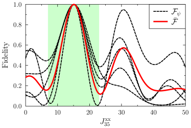
Figure 2: Average fidelity $\bar{\mathcal{F}}$ and fidelity $\mathcal{F}_{\psi}$ for some random states $\psi$ for implementing the Toffoli gate in a 4 qubit network (see discussion in the text). All the parameters are set to the optimal ones, except $J_{35}^{xx}$ in the abscissa. The region around the only global peak is filled in green.

This is indeed shown in Fig.2 with a real example for the implementation of the Toffoli gate (see the application section below). In Fig.2 the average fidelity $\bar{\mathcal{F}}$ has three local maxima at ${\boldsymbol{\lambda}}^{\rm loc.}_{k}$ ($k=1,2,3$) and a single global maximum at ${\boldsymbol{\lambda}}^{\rm gl.}$, namely the optimal parameters, while the fidelities $\mathcal{F}_{\psi}$ for different random states $\psi$ have a more complicated behavior. In view of the argument discussed above, all the state fidelities $\mathcal{F}_{\psi}$ have a global maximum at ${\boldsymbol{\lambda}}^{\rm gl.}$ while, remarkably, at least one fidelity $\mathcal{F}_{\psi}$ has no local maximum at ${\boldsymbol{\lambda}}^{\rm loc.}_{k}$. Our stochastic learning algorithm uses a gradient descent technique for locally maximising the function $\mathcal{F}_{\psi}(\boldsymbol{\lambda})$. Therefore, if we are around the slopes of a local maximum of $\mathcal{F}_{\psi}(\boldsymbol{\lambda})$ (say ${\boldsymbol{\lambda}}^{\rm loc.}_{k}$ from the previous example) and the state $\left|{\psi}\right\rangle$ is randomly changed to $\left|{\phi}\right\rangle$, that local maximum may disappear from $\mathcal{F}_{\phi}(\boldsymbol{\lambda})$ allowing the algorithm to escape from this non-optimal region when the parameters are updated via Eq.(4). On the other hand, when the algorithm is probing the neighborhood of a true optimal point for which $\bar{\mathcal{F}}(\boldsymbol{\lambda}){=}1$, (e.g. ${\boldsymbol{\lambda}}^{\rm gl.}$ in the previous example), then the maximum of $\mathcal{F}_{\psi}(\boldsymbol{\lambda})$ does not disappear when the state $\psi$ is changed, allowing the “climbing” procedure to continue.

The above stochastic algorithm may be combined with a deterministic maximization of Eq.(3). In our simulations we use stochastic learning for the initial global span of the parameter manifold and, if it reaches a suitably high fidelity (e.g. $\bar{\mathcal{F}}{>}95\%$), then it is reasonable to suppose that the algorithm has found a global maximum. Starting from this point we perform a local maximization of Eq.(3) and, if $\bar{\mathcal{F}}{\simeq}1$ is reached, the learning has been successful. Otherwise we repeat the procedure.

It is worth emphasizing that given a target gate $U$, it is an open question to understand a priori whether a solution may exist for a graph with a certain set of interactions (e.g. Heisemberg, Ising, etc.). Unlike in quantum control, where given a time dependent Hamiltonian $\mathcal{H}(t)=\mathcal{H}_{0}+\beta(t)\mathcal{V}$ one can check in advance whether $U=T[\exp({-}i\int_{0}^{1}\mathcal{H}(t)dt)]$ for some control profile $\beta(t)$: such profile can exist only if $U$ is contained in the group associated to the algebra generated by the repeated commutators of $\mathcal{H}_{0}$ and $\mathcal{V}$. Although no complete algebraic characterization is known for our case (see however the Methods for a necessary condition) and we have to study each problem numerically, in the next sections we find some structures which enable the implementation of important quantum gates. All numerical simulations have been obtained in a laptop computer using QuTiP Johansson et al. (2013).

Application: Toffoli gate

The Toffoli gate is a key component for many important quantum algorithms, notably the Shor algorithm Shor (1997), quantum error correction Cory et al. (1998), fault-tolerant computation Dennis (2001), quantum arithmetic operations Vedral et al. (1996) and, together with the Hadamard gate, is universal for quantum computation Shi (2003). Experimental implementations of this gate has been obtained with trapped ions Monz et al. (2009), superconducting circuits Reed et al. (2012); Fedorov et al. (2011), or photonic architectures Lanyon et al. (2009). Toffoli gate is a controlled-controlled-not (CCNOT) operation acting on three qubits. It can be implemented in a circuit using five two-qubit gates Nielsen and Chuang (2000), or can be obtained in coupled systems via quantum control techniques Stojanović et al. (2012); Zahedinejad et al. (2015). Efficient schemes require higher dimensional system (i.e. qudits) Lanyon et al. (2009). On the other hand, the direct implementation using natural interactions is complicated, since the Hamiltonian $\mathcal{H}_{\rm CCNOT}$ corresponding to the gate, i.e. ${\rm CCNOT}{=}e^{i\mathcal{H}_{\rm CCNOT}}$, has three-body interactions which unlikely appear in nature.

By applying our quantum hardware design procedure, we show that the Toffoli gate can be implemented in a four qubit network using only pairwise interactions and constant control fields. Our findings enable the construction of a device which implements the Toffoli gate with a fidelity $\bar{\mathcal{F}}{=}99.98\%$ by simply “waiting” for the natural dynamics to occur, without the need of external control pulses.

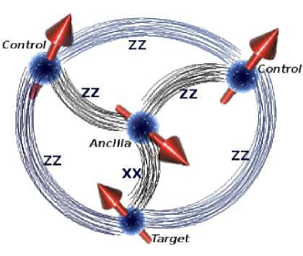
Figure 3: Network implementing the Toffoli gate. The gate acts on the three external qubits (the top ones being the control qubits, and the bottom one being the target), and has an additional auxiliary qubit in the center.

We consider a four qubit network as displayed in Fig. 3, where the control qubits are labeled by the indices 1,2, the target is qubit 3 and the ancilla is qubit 4. We start our analysis by considering a fully-connected graph where each qubit interacts with the others using XX- and ZZ-type pairwise interactions, as this kind of interaction can be obtained in superconducting circuits Geller et al. (2014). Because of the symmetries of the Toffoli gate (see Methods), we consider the two control qubits to be equally coupled to the target and the ancilla: $J^{\alpha\beta}_{1m}{=}J^{\alpha\beta}_{2m}$, for $m{=}3,4$ and similarly we set $h^{\alpha}_{1}{=}h^{\alpha}_{2}$. Moreover, since the Toffoli gate is real, we only consider local fields in the X and Z directions and set $\left|{\psi_{A}}\right\rangle{=}\cos\eta\left|{\uparrow}\right\rangle{+}e^{i\xi}\sin\eta\left|{\downarrow}\right\rangle$. By combining SGD with the maximization of Eq.(3) we find the following optimal parameters,

$$J^{zz}_{12} =-8.940, J^{zz}_{13} =-4.957, J^{zz}_{14} =-5.657,$$

$$h^{z}_{1} =-2.428, h^{z}_{3} =J^{zz}_{13}, h^{z}_{4} =-0.165,$$

$$h^{x}_{3} =-19.08, h^{x}_{4} =-4.267, J^{xx}_{34} =15.06,$$

$$\eta =0.8182, \xi =0.0587,$$ (5)

where the other XX- and ZZ-type interactions not displayed in (5) are found to be zero by the learning algorithm, so the optimal configuration is the one summarized in Fig.3 where the XX coupling is only between qubits 3 and 4. In more physical terms, if the maximal allowed coupling is fixed to $J/2\pi{\approx}40{\rm MHz}$, then we find a gate time of $60{\rm ns}$ and

$$J^{zz}_{12} =-149.2\,{\rm MHz}, J^{zz}_{13} =-82.71\,{\rm MHz},$$

$$J^{zz}_{14} =-94.39\,{\rm MHz}, J^{xx}_{34} =251.3\,{\rm MHz},$$

$$h^{x}_{3} =-318.4\,{\rm MHz}, h^{x}_{4} =-71.2\,{\rm MHz},$$

$$h^{z}_{1} =-40.52\,{\rm MHz}, h^{z}_{4} =-2.751\,{\rm MHz},$$

$$h^{z}_{3} =J^{zz}_{13}.$$ (6)

With the optimal parameters of Eqs.(5),(6) we obtain an average gate fidelity of 99.98%, above the threshold for topological fault tolerance for single- and two-qubit gates, while by avoiding the extra phase fixing $\xi{=}0$ we still obtain $\bar{\mathcal{F}}{=}99.92\%$. Moreover, our gate fidelity is above the Toffoli gate accuracy threshold ($755/756{\simeq}99.87\%$) for fault-tolerant computation in the limit in which Clifford gate errors are negligible Gaitan (2008).

The optimal parameters (5),(6) are stable against an imperfect tuning of the interactions. Indeed, we considered a perturbation $\lambda_{k}{\to}\lambda_{k}{+}\epsilon r_{k}$, $r_{k}{\in}[0,1]$ being a random number and $\epsilon$ being the strength of the static perturbation, and found that $\bar{\mathcal{F}}{>}99.9\%$ if $\epsilon{<}0.04$ ($\epsilon{<}0.7\,{\rm MHz})$ and $\bar{\mathcal{F}}{>}99\%$ if $\epsilon{<}0.18$ ($\epsilon{<}3\,{\rm MHz})$.

Application: Fredkin gate

Fredkin gate is a controlled-swap (CSWAP) operation acting on three qubits which is universal for reversible computation Nielsen and Chuang (2000). We found that this gate can be obtained with perfect fidelity (up to the numerical precision) in a four qubit network with Hamiltonian (1) where $J^{xx}_{12}{=}J^{xx}_{13}{=}13.60$ $(227.0\,{\rm MHz})$, $J^{\alpha\alpha}_{23}{=}{-}4.712$ $(-78.62\,{\rm MHz})$, $J^{xx}_{24}{=}J^{xx}_{34}{=}8.400$ $(140.2\,{\rm MHz})$, $J^{zz}_{12}{=}J^{zz}_{13}{=}11.15$ $(186.1\,{\rm MHz})$, $h^{x}_{4}{=}1.025$ $(17.11\,{\rm MHz})$, $h^{z}_{1}{=}\pi$ $(54.42\,{\rm MHz})$. The values in MHz correspond to a gate time of 60ns. Moreover, $e^{{-}i\mathcal{H}}{=}{\rm CSWAP}_{123}{\otimes}U_{4}$ so the gate is independent on the initial state of the ancilla. As for the Toffoli gate, this optimal configuration has been obtained by starting the training procedure with a fully connected graph with all the interactions, so the fact that some interactions are zero is a result of the optimization process.

Application: remote logic

We study a qubit network which implements a maximally entangling gate between two sites which are not directly coupled. Remote logic has been studied extensively in spin chains for achieving entangling operations between the boundary sites Banchi et al. (2011); Yao et al. (2013); Banchi et al. (2015); Benjamin and Bose (2003), and it is a building block for a proposed architecture for solid-state quantum computation at room temperature Yao et al. (2012). For simplicity we consider a SU(2) invariant four qubit network, interacting with a Heisenberg Hamiltonian $H{=}\sum_{i{\neq}j=1}^{4}\sum_{\alpha{=}x,y,z}J_{ij}\sigma_{i}^{\alpha}\sigma_{j}^{\alpha}/4$ where there is no direct coupling between qubits 1 and 4 ($J_{14}{=}0$). Applying our learning algorithm we found that the $\sqrt{\rm SWAP}$ gate, which is universal for quantum computation when paired with single qubit operations Nielsen and Chuang (2000), can be achieved between qubits 1 and 4 with unit fidelity with different choices of $J_{12}{=}J_{24}$, $J_{13}{=}J_{34}$, and $J_{23}$ when the initial state of ancillae is $(\left|{\uparrow\downarrow}\right\rangle{-}\left|{\downarrow\uparrow}\right\rangle)/\sqrt{2}$. Given this simplification one can then find a solution analytically: $J_{12}{=}\alpha{+}\pi\sqrt{(2n)^{2}{-}1}{/}\sqrt{8}$, $J_{13}{=}\alpha{-}\pi\sqrt{(2n)^{2}{-}1}{/}\sqrt{8}$, $J_{23}{=}\alpha+(-1)^{n}\pi$, where $n$ is an integer. We find analytically that irrespective of $\alpha$ the above choice gives perfect fidelity. Our strategy has not found any three-qubit configurations which implement a remote $\sqrt{\rm SWAP}$ gate, so the four qubit network is the minimal non-trivial example. Remarkably, some of our 4-qubit configuration are more stable to noise than the direct implementation of the gate in a two-qubit system (namely when $J_{14}{=}\pi/2$ and the other couplings are zero). For instance, if $J_{ij}=J_{ij}^{\rm optimal}+\epsilon$, $J_{ij}^{\rm optimal}$ being the optimal value for implementing the gate, we found that when $\epsilon$ is randomly distributed in $[0,1/2]$, then the 4-qubit system with $n=1$ still has, on average, $\bar{\mathcal{F}}\simeq 99.1\%$, while the direct two-qubit case has $\bar{\mathcal{F}}\simeq 98.8\%$.

Towards a scalable architecture for quantum computation

Current architectures for quantum computation, e.g. with superconducting qubits Barends et al. (2014) or ion traps Monz et al. (2016), are based on an arrays of interacting qubits which are continuously controlled via external pulses to implement the desired operation. This approach may suffer from scalability issues because, even assuming the ability to maintain quantum coherence for a long time, extremely large (classical) control units will be necessary to generate the sophisticated pulse sequences required to implement a full-scale quantum algorithm. On the other hand, the approach that we have in mind shares more similarities with integrated circuits in nowadays electronics, where a set of special-purpose logic units (modules) are wired together to achieve computation (or other tasks). In our vision, different modules can be fabricated with qubit networks designed to produce a specific logic task, namely a quantum gate, automatically without the need of external control. As in Fig.1 the different logic and memory units can be reciprocally connected using a quantum bus, whose purpose is to transfer the qubit states between the quantum registers/memory and the input/output qubits of the modules. In Fig.1 for simplicity the input/output ports of the modules are designed in the same physical qubits, although this can be easily extended to more general cases. The quantum bus can be realized with different technologies, e.g. with microwave resonators Mariantoni et al. (2011), or can also be implemented via quantum state transfer in a qubit network Nikolopoulos and Jex (2014). The modules shown in Fig.1 can be designed to produce either simple basic operations, like the CNOT or the Toffoli gate, or, in principle, they can directly implement larger components of a quantum algorithm like the Quantum Fourier Transform or error correcting codes Nielsen and Chuang (2000). In this respect, to treat systems with many parameters one can easily combine our optimization strategy, based on fidelity statistics, with metaheuristic strategies Storn and Price (1997) which simultaneously deals with many candidate solutions and are known to be fast in global optimization with high-dimensional parameter spaces. Moreover, highly optimized deep learning algorithms are already used to train neural networks with 60 millions of parameters Krizhevsky et al. (2012). However, given the difficulty in numerically simulating large quantum systems, this approach may be reasonable for networks up to, say, 20-30 qubits.

Discussion

Inspired by classical supervised learning, we have proposed an optimization scheme to encode a quantum operation into the unmodulated dynamics of a qubit register, which is part of a bigger network of pairwise interacting qubits. Our strategy is based on the static engineering of the pairwise couplings, and enables the creation of a quantum device which implements the desired operation by simply waiting for the natural dynamics to occur, without the need of external control pulses. Our findings show that machine learning inspired techniques can be combined with quantum mechanics not only for data classification speed-up Rebentrost et al. (2014); Wittek (2014) or quantum black-box certification Bisio et al. (2010); Wiebe et al. (2014), but also for quantum hardware design.

This paper opens up the topic of encoding quantum gates and operations into the unmodulated dynamics of qubit networks. Although we have focused on small systems, larger networks can be considered using more efficient training schemes. These would enable the simulation of larger components of a quantum algorithm, since different multi-qubit gates can be combined into a unique quantum operation which can be simulated in a large quantum network. Moreover, when combined with a quantum bus as in Fig. 1, our strategy can provide an alternative approach to universal quantum computation which avoids the decomposition of the algorithm into one- and two-qubit gates. Note that most quantum algorithms take classical inputs so the extra control required for initialization demands the further ability to fully polarise globally the spins. The latter step is however typically much easier than the implementation of entangling gates, which has been considered in this paper. Moreover, in view of the recent experimental measures of the average gate fidelity Lu et al. (2015), it is tempting to predict an all-quantum version of our learning procedure where $\bar{\mathcal{F}}$ is not classically simulated, but rather directly measured. This would require a further highly controlled system to infer the optimal parameters of an uncontrolled quantum network, which can be used to industrialize the production of unmodulated quantum devices implementing the desired algorithm.

Our results demonstrate the efficacy of the proposed scheme in designing four qubit networks which implement the Toffoli and Fredkin gates or remote logic operations. The proposed Toffoli gate is fast, has high-fidelity for fault-tolerant computation, and only uses static XX- and ZZ-type interactions which can be achieved in superconducting systems Geller et al. (2014). The key advantage of our method is in exploiting all the permanent interactions in the qubit network without trying to suppress some of them sequentially to implement pairwise gates. Moreover, being based on non-equilibrium dynamics, our gate is fast: if $J/2\pi{\approx}40{\rm MHz}$ then the total operation time is around $60{\rm ns}$ which matches the current gate times for single and two qubit operations Barends et al. (2014).

Methods

Learning rate

The choice of the learning rate $\epsilon$ is crucial. If the initial learning rate is too small, it might not escape from the different “local maximum” points, while if it is too large it will continue to randomly jump without even seeing the local maxima. To maximize the speed and precision of SDG the learning rate $\epsilon$ has to decrease as a function of the steps, a common choice being $\epsilon{\propto}m^{-1/2}$ where $m$ is the step counter Bottou (1998). However, when the gradient in Eq.(4) cannot be performed analytically, one can use more sophisticated techniques Spall (2005) where both the learning rate and the finite difference approximation of the gradient change as a function of $m$.

Symmetries

In the design of the quantum network and its couplings the number of parameters can be drastically reduced if the target unitary operation $U_{Q}$ has some symmetries, namely if there exists some unitary matrix $S$ such that $[U_{Q},S_{Q}]{=}0$. This condition requires the quantum channel $\mathcal{E}_{\boldsymbol{\lambda}}[\rho]{=}\operatorname*{Tr}_{A}[e^{-i\mathcal{H}}\rho{\otimes}\rho_{A}e^{i\mathcal{H}}]$ to satisfy $\mathcal{E}_{\boldsymbol{\lambda}}(S_{Q}\rho S_{Q}^{\dagger}){=}S_{Q}\mathcal{E}_{\boldsymbol{\lambda}}(\rho)S_{Q}^{\dagger}$ for each state $\rho$, e.g. $[\mathcal{H},S_{Q}{\otimes}\openone_{A}]{=}0$. Conversely, if the interaction type is fixed by nature (for instance, only Ising or Heisenberg interactions are allowed), then one has to check whether the Lie algebra spanned by the operators in $\mathcal{H}$ contains the generators of $U_{Q}$.

Bottom-up construction: Lie algebraic characterization

All the numerical results presented in the main text are obtained using a top-down approach: after selecting the interaction types (e.g. XX, ZZ, Heisenberg etc.), the algorithm starts with a zero-bias fully connected configuration where all the qubit pairs of the network interacts with all possible interactions, each weighted with a different parameter, and different local fields. As a result of the training procedure, we found numerically that most of these parameters are indeed zero. However, for larger networks it is better to use a bottom-up approach where one starts with a minimal set of parameters, and then adds other parameters until a solution is found.

To construct a minimal set of parameters one can use a Lie algebraic characterization inspired by quantum control. We write the Hamiltonian as $\mathcal{H}{=}\sum_{j}\lambda_{j}\mathcal{O}_{j}$, where $\lambda_{j}$ are the independent parameters and $\mathcal{O}_{j}$ the operators. If the parameters are time dependent, then there exist suitable pulses $\lambda_{j}(t)$ such that the dynamics implements the target gate $G$ only if $\log(G)$ is contained in the algebra generated by the repeated commutators $[\mathcal{O}_{j},[\mathcal{O}_{k},\dots]]$. Since our scheme is based on the particular choice where $\lambda_{j}(t)$ is constant, the above characterization still provides a necessary condition. As an example, we consider the Toffoli gate and the solution Eq.(5) where $\mathcal{O}_{1}{=}\sigma_{1}^{z}\sigma_{2}^{z}$, $\mathcal{O}_{2}{=}\sigma_{1}^{z}\sigma_{3}^{z}{+}\sigma_{2}^{z}\sigma_{3}^{z}{+}2\sigma_{3}^{z}$, $\mathcal{O}_{3}{=}\sigma_{1}^{z}\sigma_{4}^{z}{+}\sigma_{2}^{z}\sigma_{4}^{z}$, $\mathcal{O}_{4}{=}\sigma_{3}^{x}\sigma_{4}^{x}$, $\mathcal{O}_{5}{=}\sigma_{1}^{z}{+}\sigma_{2}^{z}$, $\mathcal{O}_{7}{=}\sigma_{4}^{z}$, $\mathcal{O}_{8}{=}\sigma_{3}^{x}$, $\mathcal{O}_{9}{=}\sigma_{4}^{x}$. It is simple to check that $\log G$ (up to an irrelevant constant factor) is contained in the algebra generated by the operators $O_{j}$, while this is not the case if the operator $\mathcal{O}_{8}$ is removed from the Hamiltonian. Therefore, no solution is possible if $\lambda_{8}{\equiv}0$.

Inspired by the above example the bottom-up approach consists in the following steps: i) based on the symmetries of the target gate and on the physically allowed interactions one defines an initial set of operators; ii) other operators are added to the set until the dynamical algebra contains $\log(G)$; iii) one starts the numerical parameter training to check for convergence (different runs may be required). Until the solution is found one then either adds new operators, or change the previous ones.

References

- Nielsen and Chuang (2000) M. A. Nielsen and I. L. Chuang, Quantum computation and quantum information (Cambridge University Press, 2000).
- Barenco et al. (1995) A. Barenco et al., Phys. Rev. A 52, 3457 (1995).
- Aharonov et al. (2008) D. Aharonov, W. Van Dam, J. Kempe, Z. Landau, S. Lloyd, and O. Regev, SIAM review 50, 755 (2008).
- Benjamin and Bose (2003) S. C. Benjamin and S. Bose, Physical review letters 90, 247901 (2003).
- Benjamin and Bose (2004) S. C. Benjamin and S. Bose, Physical Review A 70, 032314 (2004).
- Satoh et al. (2015) T. Satoh, Y. Matsuzaki, K. Kakuyanagi, W. J. Munro, K. Semba, H. Yamaguchi, and S. Saito, Physical Review A 91, 052329 (2015).
- Li et al. (2011) Y. Li, D. E. Browne, L. C. Kwek, R. Raussendorf, and T.-C. Wei, Physical review letters 107, 060501 (2011).
- Burgarth et al. (2010) D. Burgarth, K. Maruyama, M. Murphy, S. Montangero, T. Calarco, F. Nori, and M. B. Plenio, Physical Review A 81, 040303 (2010).
- Müller et al. (2011) M. Müller, D. Reich, M. Murphy, H. Yuan, J. Vala, K. Whaley, T. Calarco, and C. Koch, Physical Review A 84, 042315 (2011).
- Banchi et al. (2011) L. Banchi, A. Bayat, P. Verrucchi, and S. Bose, Physical review letters 106, 140501 (2011).
- Devoret and Schoelkopf (2013) M. Devoret and R. Schoelkopf, Science 339, 1169 (2013).
- Wallraff et al. (2004) A. Wallraff, D. I. Schuster, A. Blais, L. Frunzio, R.-S. Huang, J. Majer, S. Kumar, S. M. Girvin, and R. J. Schoelkopf, Nature 431, 162 (2004).
- Barends et al. (2013) R. Barends, J. Kelly, A. Megrant, D. Sank, E. Jeffrey, Y. Chen, Y. Yin, B. Chiaro, J. Mutus, C. Neill, et al., Physical review letters 111, 080502 (2013).
- Chen et al. (2014) Y. Chen et al., Phys. Rev. Lett. 113, 220502 (2014).
- Geller et al. (2014) M. R. Geller, E. Donate, Y. Chen, C. Neill, P. Roushan, and J. M. Martinis, arXiv preprint arXiv:1405.1915 (2014).
- Neeley et al. (2010) M. Neeley, R. C. Bialczak, M. Lenander, E. Lucero, M. Mariantoni, A. O’Connell, D. Sank, H. Wang, M. Weides, J. Wenner, et al., Nature 467, 570 (2010).
- Paik et al. (2011) H. Paik, D. Schuster, L. S. Bishop, G. Kirchmair, G. Catelani, A. Sears, B. Johnson, M. Reagor, L. Frunzio, L. Glazman, et al., Physical Review Letters 107, 240501 (2011).
- Vedral et al. (1996) V. Vedral, A. Barenco, and A. Ekert, Physical Review A 54, 147 (1996).
- Fedorov et al. (2011) A. Fedorov, L. Steffen, M. Baur, M. Da Silva, and A. Wallraff, Nature 481, 170 (2011).
- Cory et al. (1998) D. G. Cory, M. Price, W. Maas, E. Knill, R. Laflamme, W. H. Zurek, T. F. Havel, and S. Somaroo, Physical Review Letters 81, 2152 (1998).
- Bravyi et al. (2008) S. Bravyi, D. P. DiVincenzo, D. Loss, and B. M. Terhal, Phys. Rev. Lett. 101, 070503 (2008).
- Biamonte and Love (2008) J. D. Biamonte and P. J. Love, Physical Review A 78, 012352 (2008).
- Brif et al. (2010) C. Brif, R. Chakrabarti, and H. Rabitz, New Journal of Physics 12, 075008 (2010).
- Bishop (2006) C. M. Bishop, Pattern recognition and machine learning (Springer, 2006).
- Wittek (2014) P. Wittek, Quantum machine learning: what quantum computing means to data mining (Elsevier, Oxford, 2014).
- Rebentrost et al. (2014) P. Rebentrost, M. Mohseni, and S. Lloyd, Phys. Rev. Lett. 113, 130503 (2014).
- Paparo et al. (2014) G. D. Paparo, V. Dunjko, A. Makmal, M. A. Martin-Delgado, and H. J. Briegel, Physical Review X 4, 031002 (2014).
- Wiebe et al. (2015) N. Wiebe, A. Kapoor, and K. Svore, Quantum Information & Computation 15, 0318 (2015).
- Lloyd et al. (2014) S. Lloyd, M. Mohseni, and P. Rebentrost, Nature Physics 10, 631 (2014).
- Rotondo et al. (2015) P. Rotondo, M. C. Lagomarsino, and G. Viola, Physical review letters 114, 143601 (2015).
- Nagaj (2012) D. Nagaj, Physical Review A 85, 032330 (2012).
- Bang et al. (2008) J. Bang, J. Lim, M. Kim, and J. Lee, arXiv preprint arXiv:0803.2976 (2008).
- Gammelmark and Mølmer (2009) S. Gammelmark and K. Mølmer, New Journal of Physics 11, 033017 (2009).
- Magesan et al. (2011) E. Magesan, R. Blume-Kohout, and J. Emerson, Physical Review A 84, 012309 (2011).
- Pedersen et al. (2008) L. H. Pedersen, N. M. Møller, and K. Mølmer, Physics Letters A 372, 7028 (2008).
- Collins and Śniady (2006) B. Collins and P. Śniady, Communications in Mathematical Physics 264, 773 (2006).
- Bottou (1998) L. Bottou, in Online Learning and Neural Networks, edited by D. Saad (Cambridge University Press, Cambridge, UK, 1998) revised, oct 2012.
- Johansson et al. (2013) J. Johansson, P. Nation, and F. Nori, Computer Physics Communications 184, 1234 (2013).
- Shor (1997) P. W. Shor, SIAM journal on computing 26, 1484 (1997).
- Dennis (2001) E. Dennis, Physical Review A 63, 052314 (2001).
- Shi (2003) Y. Shi, Quantum Information & Computation 3, 84 (2003).
- Monz et al. (2009) T. Monz, K. Kim, W. Hänsel, M. Riebe, A. Villar, P. Schindler, M. Chwalla, M. Hennrich, and R. Blatt, Physical review letters 102, 040501 (2009).
- Reed et al. (2012) M. Reed, L. DiCarlo, S. Nigg, L. Sun, L. Frunzio, S. Girvin, and R. Schoelkopf, Nature 482, 382 (2012).
- Lanyon et al. (2009) B. P. Lanyon, M. Barbieri, M. P. Almeida, T. Jennewein, T. C. Ralph, K. J. Resch, G. J. Pryde, J. L. O’Brien, A. Gilchrist, and A. G. White, Nature Physics 5, 134 (2009).
- Stojanović et al. (2012) V. M. Stojanović, A. Fedorov, A. Wallraff, and C. Bruder, Physical Review B 85, 054504 (2012).
- Zahedinejad et al. (2015) E. Zahedinejad, J. Ghosh, and B. C. Sanders, Physical Review Letters 114, 200502 (2015).
- Gaitan (2008) F. Gaitan, Quantum error correction and fault tolerant quantum computing (CRC Press, 2008).
- Yao et al. (2013) N. Y. Yao, Z.-X. Gong, C. R. Laumann, S. D. Bennett, L.-M. Duan, M. D. Lukin, L. Jiang, and A. V. Gorshkov, Physical Review A 87, 022306 (2013).
- Banchi et al. (2015) L. Banchi, E. Compagno, and S. Bose, Physical Review A 91, 052323 (2015).
- Yao et al. (2012) N. Y. Yao, L. Jiang, A. V. Gorshkov, P. C. Maurer, G. Giedke, J. I. Cirac, and M. D. Lukin, Nature communications 3, 800 (2012).
- Barends et al. (2014) R. Barends, J. Kelly, A. Megrant, A. Veitia, D. Sank, E. Jeffrey, T. White, J. Mutus, A. Fowler, B. Campbell, et al., Nature 508, 500 (2014).
- Monz et al. (2016) T. Monz, D. Nigg, E. A. Martinez, M. F. Brandl, P. Schindler, R. Rines, S. X. Wang, I. L. Chuang, and R. Blatt, Science 351, 1068 (2016).
- Mariantoni et al. (2011) M. Mariantoni et al., Science 334, 61 (2011).
- Nikolopoulos and Jex (2014) G. M. Nikolopoulos and I. Jex, Quantum State Transfer and Network Engineering (Springer, 2014).
- Storn and Price (1997) R. Storn and K. Price, Journal of global optimization 11, 341 (1997).
- Krizhevsky et al. (2012) A. Krizhevsky, I. Sutskever, and G. E. Hinton, in Advances in Neural Information Processing Systems 25, edited by F. Pereira, C. J. C. Burges, L. Bottou, and K. Q. Weinberger (Curran Associates, Inc., 2012) pp. 1097–1105.
- Bisio et al. (2010) A. Bisio, G. Chiribella, G. M. D’Ariano, S. Facchini, and P. Perinotti, Physical Review A 81, 032324 (2010).
- Wiebe et al. (2014) N. Wiebe, C. Granade, C. Ferrie, and D. Cory, Physical review letters 112, 190501 (2014).
- Lu et al. (2015) D. Lu, H. Li, D.-A. Trottier, J. Li, A. Brodutch, A. P. Krismanich, A. Ghavami, G. I. Dmitrienko, G. Long, J. Baugh, et al., Physical review letters 114, 140505 (2015).
- Spall (2005) J. C. Spall, Introduction to stochastic search and optimization: estimation, simulation, and control, Vol. 65 (John Wiley & Sons, 2005).