UCB-PTH-15/08

Flat-space Quantum Gravity in AdS/CFT

Yasunori Nomura, Fabio Sanches, and Sean J. Weinberg

Berkeley Center for Theoretical Physics, Department of Physics,
University of California, Berkeley, CA 94720, USA

Theoretical Physics Group, Lawrence Berkeley National Laboratory, CA 94720, USA

1 Introduction

Quantum gravity has been elusive so far. Our lack of understanding manifests itself especially prominently in the study of black hole physics, where basic questions such as unitarity of the evolution and the smoothness of horizons are still under debate [1, 2, 3]. Ever since the discovery of the thermodynamic behavior of black holes [4, 5, 6], we have been searching for the deeper structure of spacetime and gravity beyond that described by general relativity. In fact, we may need to revise the concept of spacetime itself, as suggested by the holographic principle [7, 8] and complementarity hypothesis [9, 10]. Furthermore, it seems that a perturbative approach to gravity is incapable of revealing the real nature of spacetime.

AdS/CFT duality [11, 12] provides a possible approach to quantum gravity at the nonperturbative level, albeit in spacetimes that are asymptotically AdS. Motivated by the task of understanding microscopic dynamics of an evolving black hole, the first half of this paper presents a scheme which can describe quantum gravitational processes in asymptotically flat spacetime using CFTs. A key point is that this does not require a true (holographic) theory of quantum gravity in asymptotically flat spacetime, i.e. one accommodating the full Bondi-Metzner-Sachs symmetry at null infinity [13] and giving a fully unitary $S$-matrix in the asymptotically flat spacetime. Instead, we can describe flat-space quantum gravitational processes by focusing on time scales sufficiently shorter than the AdS time scale and in a sufficiently central region of the global AdS space in a single AdS volume at the center. This description can be made extremely (and perhaps infinitely) accurate by making the AdS length scale large compared to the scale of interest.

The relevant Heisenberg-picture states in the gravitational bulk are represented by CFT operators at the point corresponding to the infinite past, which exists on the flat Euclidean space obtained by conformally compactifying the boundary spacetime in which the CFT originally lived. We need not use the concept of CFT fields: knowing the spectrum and algebra of these operators is enough to understand the dynamics of our interest. In particular, by identifying the dilatation $D$ of the conformal symmetry with time translation in the bulk, we can describe continuous time evolution (not just an $S$-matrix type quantity) in the gravitational bulk. Since the CFT description eliminates all the gauge redundancies in the gravitational theory (including those associated with the holographic reduction of degrees of freedom), this provides a fully gauge-fixed description of physical observables in quantum gravity. Our particular choice of identifying $D$ as time translation corresponds to taking the reference clock to be in the asymptotic region [14].

Despite its conceptual simplicity, current theoretical technology does not allow us to compute the physics of black holes explicitly by following the above program. In the second half of this paper, we therefore adopt a different strategy and use information from the gravitational description to study what properties the dual CFTs must possess. In particular, we describe how the picture of an evaporating black hole in Refs. [15, 16], proposed to solve the black hole information problem [1, 3], is translated into the CFT language given here. This has at least two virtues. First, since the physics of black holes is expected to be universal, the structures we identify can be viewed as predictions for nonperturbative properties of the CFTs that have weakly coupled gravitational descriptions. In principle, this allows us to test (aspects of) the picture of Refs. [15, 16], perhaps with some future theoretical developments. Second, the translated CFT description clarifies the concept of spacetime-matter duality introduced in Refs. [15, 16]: the black hole microstates play roles of both spacetime and matter, but in fact are neither. In the CFT language, this can be stated as properties exhibited by the operators corresponding to black hole microstates.

The emergence of spacetime and gravity in AdS/CFT is an important subject, and it has been studied by many authors from various different angles, e.g., in Refs. [17, 18, 19, 20, 21, 22, 23, 24, 25, 26, 27, 28, 29, 30, 31, 32]. Our analysis builds on many of these works, which we refer to more explicitly as we go along. It asserts that when a relevant CFT possesses a finite central charge, which is necessary to describe nonperturbative gravitational processes in the bulk, the sector allowing for a semiclassical particle interpretation comprises only a tiny subset of the whole degrees of freedom representing the single AdS volume. This elucidates why, in contrast with what is postulated in Refs. [3, 33, 34, 35], the microscopic information about a black hole cannot be viewed as propagating in semiclassical spacetime in the near black hole region.

The organization of this paper is as follows. In Section 2, we present the scheme which describes flat-space quantum gravitational processes using CFTs. We discuss under what conditions and to what extent the CFTs may provide such descriptions and how the continuous time evolution picture in the gravitational bulk arises from the algebra of CFT operators defined at a point in Euclidean spacetime. We then discuss in Section 3 how these quantum gravitational processes may be physically interpreted (purely) in CFTs. This requires us to decompose operators into smaller elements, which corresponds to decomposing the Hilbert space of the states for the “entire universe” into those for smaller subsystems. We discuss how this can be done using the operator product expansion (OPE), defined as the action of operators on general states. We finally apply the scheme to black hole states to see how the picture of Refs. [15, 16] may be realized in CFTs. Section 4 is devoted to the summary and discussion.

2 Embedding Asymptotically Flat Spacetime in AdS/CFT

One goal of this paper is to use AdS/CFT duality to study how the structure of (a class of) CFTs encodes the physics of an evaporating, dynamically formed black hole. As a first step, here we ask how the physics of flat-space quantum gravity may be encoded in CFTs.

Throughout the paper, we focus on the class of CFTs whose dual descriptions possess energy intervals in which physics is well described by weakly coupled effective field theories with Einstein gravity in spacetimes one dimension higher than those of the corresponding CFTs. Specifically, for a $d$-dimensional CFT, we require that the dual theory has

$$l_{\rm P}<l_{\rm s}<R_{\rm c}\ll R,$$ (1)

where $l_{\rm P}$, $l_{\rm s}$, and $R$ are the $(d+1)$-dimensional Planck length, string length, and AdS curvature length, respectively, and $R_{\rm c}$ collectively represents characteristic length scales associated with compact extra dimensions beyond $d+1$ spacetime dimensions. The precise and general conditions for a CFT to give such descriptions are not yet understood, although some necessary and/or sufficient conditions to have weakly coupled dual gravitational descriptions have been discussed in various contexts [21, 24, 27, 31]. In this paper, we assume the existence of the relevant CFTs.

Since the flat-space limit corresponds to length scales smaller than the AdS radius $R$, we are interested only in a single AdS volume. We choose to work in global AdS spacetime, focusing on a single AdS volume at the center. This has the virtue that we need not be concerned with the Poincaré horizon in dual AdS_d+1 descriptions. In particular, we take our CFTs to live in ${\bf S}^{d-1}\times{\bf R}$, where ${\bf S}^{d-1}$ represents the $(d-1)$-dimensional sphere with radius $R$.

2.1 AdS radius as an IR and UV cutoff

AdS/CFT duality is believed to hold between a $d$-dimensional CFT and string theory on a spacetime whose asymptotic region contains an AdS_d+1 factor. Suppose the spacetime geometry in the string theory side is asymptotically AdS${}_{d+1}\times X$, where $X$ is a compact space. It seems possible to make $X$ as small as of order the AdS radius $R$. This was indeed the case in originally discussed examples of AdS/CFT [11], and we do not anticipate any obstacles keeping $X$ this size (or smaller) in more elaborate setups, for example in nonsupersymmetric cases. This allows us to dimensionally reduce on $X$, yielding theory in AdS_d+1 that contains Kaluza-Klein towers associated with $X$. In this subsection we work in this framework.

Let us consider a single AdS volume $V$ at the center of the bulk at some time $\tau=t_{0}$:

$$0\leq r<R,$$ (2)

where $\tau$ and $r$ are the AdS time and radial coordinates defined by the metric

$$ds^{2}=-\biggl{(}1+\frac{r^{2}}{R^{2}}\biggr{)}\,d\tau^{2}+\frac{dr^{2}}{1+\frac{r^{2}}{R^{2}}}+r^{2}d\Omega^{2}.$$ (3)

This region serves as our proxy of (an equal-time hypersurface of) flat space, in which $R$ plays the role of the IR cutoff. When we refer to flat-space physics, we mean physical processes occurring in (a sufficiently interior part of) this region; see Fig. 1. In general, excitations involved in these processes modify the metric in Eq. (3), in which case the choice of time slice, $\tau=t_{0}$, refers to that at the boundary of the region, $\partial V$.

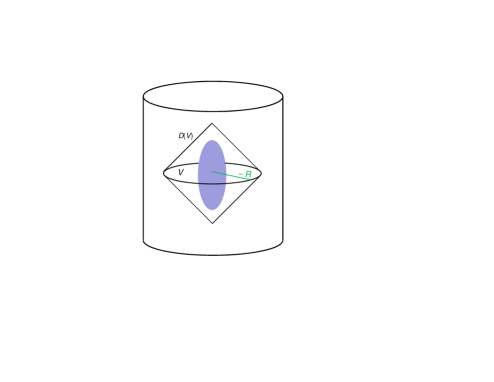
Figure 1: A single AdS volume $V$ is selected at the center of the global AdS space at some reference time $t_{0}$. We are concerned with processes occurring in a sufficiently inner region of the domain of dependence of $V$, $D(V)$.

What are the CFT operators representing physical configurations in the volume $V$ (or more precisely, in the region inside $\partial V$)? Imagine that the CFT is defined on a flat $d$-dimensional Euclidean spacetime obtained by performing a Weyl transformation on (Euclideanized) ${\bf S}^{d-1}\times{\bf R}$ and adding a point, $x=x_{-\infty}$, corresponding to $\tau=-\infty$. Here, $x$ represents the coordinates of the $d$-dimensional space in which the CFT lives. We may then define the set of (gauge-invariant) operators acting at this point, $\Psi$’s, which corresponds to all the elements of the Hilbert space of this CFT in radial quantization. The CFT state created by any of these operators, $\Psi|0\rangle_{\rm CFT}$, then corresponds to a Heisenberg state in the gravitational theory, representing a full spacetime history in the bulk. We can then ask what subset of these CFT operators provides a complete basis $\{\Psi_{A=1,2,\cdots}\}$ for the bulk states that can be interpreted as having excitations only in the region inside $\partial V$ at time $t_{0}$.

Let us recall that AdS/CFT relates the central charge $c$ of the CFT with the AdS radius and the $(d+1)$-dimensional Planck length as

$$c\sim\left(\frac{R}{l_{\rm P}}\right)^{d-1}.$$ (4)

Since we are interested in physics in (large) flat spacetime, we take $R\gg l_{\rm P}$. Namely, we are considering CFTs with

$$c\gg 1.$$ (5)

In general, a CFT operator $\Psi$ is given by a superposition of primary and descendant operators ${\cal O}_{I}$:

$$\Psi=\sum_{I}\alpha_{I}\,{\cal O}_{I}.$$ (6)

Here, ${\cal O}_{I}$’s are defined by the dilatation $D$ and special conformal transformations $K^{\mu}$ whose center is at $x=x_{-\infty}$, and we take their normalization such that the states created by them are appropriately normalized in Lorentzian ${\bf S}^{d-1}\times{\bf R}$:

$$\langle 0|{\cal O}_{I}^{\dagger}{\cal O}_{J}|0\rangle=\delta_{IJ},$$ (7)

where $|0\rangle$ is the CFT vacuum state. (This requires unconventional relative normalizations between primary and descendant operators within a single conformal multiplet.) According to AdS/CFT, the dimension $\Delta$ of a CFT (primary or descendant) operator ${\cal O}$ is related with the bulk quantities as

$$\Delta\sim ER,$$ (8)

where $E$ is the energy of the bulk state corresponding to ${\cal O}$ as measured with respect to $\tau$.

The relations in Eqs. (4, 8) imply that a CFT operator $\Psi$ containing a primary or descendant operator with $\Delta>c$ corresponds to a bulk state involving a component with $E>R^{d-2}/l_{\rm P}^{d-1}$. Such an operator cannot be an element of the basis $\{\Psi_{A}\}$ we look for, since energies this large cannot fit into $V$—they would lead to large black holes, whose Schwarzschild radii are larger than $R$. A basis element of $\{\Psi_{A}\}$ thus can be written as

$$\Psi_{A}=\sum_{I\in\{I|\Delta_{I}<c\}}\!\!\alpha_{A,I}\,{\cal O}_{I},$$ (9)

where

$$\sum_{I}\alpha_{A,I}^{*}\alpha_{B,I}=\delta_{AB}.$$ (10)

Note that the coefficients $\alpha_{A,I}$ depend on $t_{0}$, and $\alpha_{A,I}^{*}$ refers to the complex conjugate of $\alpha_{A,I}$ in Lorentzian ${\bf S}^{d-1}\times{\bf R}$.

The set of CFT operators $\Psi_{A}$ is smaller than the set spanned by all possible independent linear combinations of ${\cal O}_{I}$’s with $\Delta_{I}<c$. This is because some of these linear combinations correspond to bulk states in which not all the excitations are confined within $\partial V$ at time $t_{0}$. While an explicit expression for the sets of $\alpha_{A,I}$’s giving correct basis operators, $\Psi_{A}$, is not known, they must be uniquely determined (up to basis changes and IR ambiguities discussed in footnote 1) once the theory is fixed and time $t_{0}$ is chosen, since the CFT construction here selects time slicing in the bulk. Note that the choice of $t_{0}$ is simply a convention for how we embed our “flat spacetime” into the AdS spacetime. We refer to the set of basis operators determined in this way as ${\cal B}$:

$${\cal B}=\{\Psi_{A}\}.$$ (11)

This set contains complete information about physics occurring in our “flat spacetime,” i.e. (a sufficiently small part of) the domain of dependence of $V$, $D(V)$ (see Fig. 1).

We stress that the dimensions of operators comprising $\Psi_{A}$’s are bounded both from below (by the unitarity bound) and above (by $c$); namely, the AdS radius provides a cutoff both in the IR and UV. In fact, for finite $R$ (in units of $l_{\rm P}$), the number of elements of ${\cal B}$, $N_{\cal B}$, is finite—the holographic principle states that [7, 8, 36]

$$\ln N_{\cal B}=\frac{\Omega_{d-1}}{4}\left(\frac{R}{l_{\rm P}}\right)^{d-1}\sim c,$$ (12)

where $\Omega_{d-1}=2\pi^{d/2}/\Gamma(d/2)$ is the volume of the unit $(d-1)$-sphere, and we have used Eq. (4). This is the CFT statement for holography in flat spacetime, in which (unlike a large AdS region) a volume does not scale as the area surrounding it.

2.2 Flat-space quantum gravity in $d+1$ dimensions

We now discuss in more detail how we may extract physics of flat-space quantum gravity. We begin by considering the (potentially hypothetical) situation in which the compact space $X$ can be completely ignored. Specifically, we consider the case in which the gravitational theory contains only two length scales

$$\tilde{l}_{\rm P}\sim l_{\rm s}\sim R_{\rm c}\ll R.$$ (13)

Here, $\tilde{l}_{\rm P}$ is the Planck length in AdS${}_{d+1}\times X$, which is related with the $(d+1)$-dimensional Planck length, $l_{\rm P}$, by

$$l_{\rm P}^{d-1}=\frac{\tilde{l}_{\rm P}^{d+n-1}}{V_{X}},$$ (14)

where $n$ and $V_{X}$ are the dimension and volume of $X$, respectively. (Here we take $V_{X}=R_{\rm c}^{n}\sim l_{\rm s}^{n}$, so that $\tilde{l}_{\rm P}\sim l_{\rm P}$.) As we will discuss below, this setup might not be realized in a consistent theory of quantum gravity (and so as a dual description of a CFT). However, it provides a useful starting point for our discussion.

Suppose we take the limit in which the cutoff for flat-space physics is removed, $R/l_{\rm P}\rightarrow\infty$, which corresponds to $c\rightarrow\infty$. The relations in Eqs. (4, 8) then imply that trans-Planckian physics in the bulk is encoded in the structure of operators with extremely large (infinite) dimensions

$$\Delta\gtrsim c^{\frac{1}{d-1}}.$$ (15)

As we have seen before, operators with $\Delta\gtrsim c$ do not correspond to physics in flat spacetime—they represent intrinsically AdS physics. This implies that physics of flat-space black holes is encoded in operators with

$$c^{\frac{1}{d-1}}\lesssim\Delta\lesssim c.$$ (16)

In the rest of this paper, we assume $d>2$.

A main point of the above discussion is that to study physics of flat-space quantum gravity, in particular that of black holes, we need to analyze the structure of operators that have very large dimensions, scaling as positive powers in $c$. The detailed range of operator dimensions on which we need to focus, however, depends on the size (and shape) of the extra dimensions as well as the physics we are interested in. Below, we discuss the effect of extra dimensions on this issue. In particular, we discuss what strategy one may adopt in studying flat-space black holes using AdS/CFT.

Let us ask how small a compact space $X$ can actually be. From the viewpoint of effective AdS_d+1 field theory, there is no restriction on the size of $X$. In particular, there is nothing wrong in taking $V_{X}\sim l_{\rm s}^{n}$ so that Eq. (13) is satisfied. However, nonperturbative effects of quantum gravity may impose constraints on the size and shape of $X$. For example, Ref. [37] argues that for $d=4$ and $n=5$ the volume of $X$ must satisfy $(V_{X}/l_{\rm s}^{5})\gtrsim g_{\rm s}(R/l_{\rm s})$, where $g_{\rm s}$ is the string coupling. A naive extension of this to arbitrary $d$ and $n$ gives

$$\frac{V_{X}}{l_{\rm s}^{n}}\gtrsim g_{\rm s}\frac{R}{l_{\rm s}}.$$ (17)

If bounds like this indeed exist, we will not be able to have a consistent setup in which the effect of extra dimensions can be completely neglected.

How do we study flat-space black holes in such cases? One way would be to consider a setup in which the extra dimensions are large, e.g. of order the AdS radius $R$, and investigate $(d+n+1)$-dimensional physics at length scales smaller than $R$. This, however, might allow us to study only special classes of black holes, e.g. those in 10- or 11-dimensional spacetimes with a large number of supersymmetries (see, e.g., Ref. [38]). Another possibility is to make $X$ as small as possible and study black holes larger than $X$. Imagine that $X$ can indeed saturate the bound in Eq. (17) with all the length scales being roughly comparable. The compactification length $R_{\rm c}\sim V_{X}^{1/n}$ is then given by

$$R_{\rm c}\sim\left(\frac{g_{\rm s}^{d-n+1}}{c^{n-1}}\right)^{\frac{1}{dn}}R.$$ (18)

The Schwarzschild radius of a black hole of mass $M$ is larger than $R_{\rm c}$ if

$$M\gtrsim M_{\rm min}\sim\left(g_{\rm s}^{(d-2)(d-n+1)}c^{d+2n-2}\right)^{\frac{1}{dn}}\frac{1}{R}.$$ (19)

This implies that we can study physics of flat-space black holes in $(d+1)$-dimensional spacetime by analyzing CFT operators with the dimensions $\Delta$ satisfying

$$M_{\rm min}R\lesssim\Delta\lesssim c.$$ (20)

For $d=4$ and $n=5$, for example, we may investigate CFT operators with

$$c^{\frac{3}{5}}\lesssim\Delta\lesssim c,$$ (21)

to study 5-dimensional flat-space black holes; see Fig. 2.

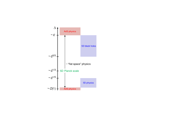
Figure 2: For AdS${}_{5}\times X_{5}$, the 5-dimensional Planck scale in the bulk corresponds to the scaling dimension of order $c^{1/3}$ in the 4-dimensional dual CFT. If there is a lower bound on the size of $X_{5}$ as suggested by the argument in Ref. [37], then (assuming $X_{5}$ has only a single scale) the physics of 5-dimensional black holes can be explored by considering operators with dimensions between $\sim c^{3/5}$ and $\sim c$. (To study 5-dimensional perturbative processes, we may focus on operators with dimensions $\lesssim c^{1/5}$.)

Bounds on $R_{\rm c}$ as the ones described above, if they indeed exist, provide a restriction on how much our minimal formalism in the previous subsection can capture flat-space physics. Consider a black hole of mass $M$ in AdS_d+1, whose Schwarzschild radius is smaller than $R$ (so that it behaves as a flat-space black hole). It has the Hawking temperature

$$T_{\rm H}(M)=\frac{d-2}{4\pi}\biggl{[}\frac{(d-1)\Omega_{d-1}}{16\pi}\biggr{]}^{\frac{1}{d-2}}\frac{1}{(Ml_{\rm P}^{d-1})^{\frac{1}{d-2}}},$$ (22)

so that a black hole with an initial mass $M_{0}$ has the lifetime of order

$$\tau(M_{0})\sim\bigl{(}M_{0}^{d}l_{\rm P}^{2(d-1)}\bigr{)}^{\frac{1}{d-2}}.$$ (23)

In order for our minimal scheme to be able to describe the full formation and evaporation history of this black hole, $\tau(M_{0})$ must be smaller than order $R$, yielding the condition for the Schwarzschild radius of the initial black hole $R_{0}=[16\pi M_{0}l_{\rm P}^{d-1}/(d-1)\Omega_{d-1}]^{1/(d-2)}$ as

$$R_{0}\lesssim\bigl{(}Rl_{\rm P}^{d-1}\bigr{)}^{\frac{1}{d}}.$$ (24)

For AdS${}_{5}\times X_{5}$, this gives $R_{0}\lesssim R^{1/4}l_{\rm P}^{3/4}$, which is inconsistent with the bound on $R_{\rm c}$ in Eq. (18), $R_{\rm c}\gtrsim R^{2/5}l_{\rm P}^{3/5}$, obtained under the assumption that $X_{5}$ has a single length scale.

This restriction does not affect the description of the Hawking emission process in flat-space quantum gravity using the scheme of Section 2.1—we can still form a black hole whose Schwarzschild radius is larger than the lower bound on $R_{\rm c}$ and study how it emits Hawking quanta. It does, however, prevent us from obtaining the full $S$-matrix elements between the initial collapsing matter and final Hawking quanta within the minimal scheme. To obtain the $S$-matrix elements, one would need to modify the minimal scheme. This can be done, for example, by introducing absorptive boundary conditions at $r\sim R$ for $\tau>t_{0}$ by adiabatically turning on couplings between the dual CFT to another larger theory at $\tau\sim t_{0}$ through appropriate CFT operators (i.e. by introducing such couplings in the appropriate region in the $d$-dimensional Euclidean spacetime). This would allow us to study the full evolution of a $(d+1)$-dimensional black hole, except for the last moment of evaporation where the physics is $(d+n+1)$-dimensional.

Our main interest in the rest of this paper is not to obtain the full $S$-matrix elements, so we will not be concerned with this issue. (Furthermore, it seems possible to circumvent the problem.) We take the viewpoint that the scheme described thus far indeed works so that we can study evaporating flat-space black holes in $d+1$ dimensions using AdS/CFT duality.

2.3 Time evolution

How can we describe time evolution in our (IR cut-off) flat spacetime? Recall that the set of CFT operators ${\cal B}$ in Eq. (11) provides a complete basis for describing a single AdS volume at the center at $\tau=t_{0}$. More precisely, a state representing a physical configuration in the region within the codimension-2 hypersurface $\partial V$ defined at $\tau=t_{0}$ can be written in general as

$$|f\rangle=\sum_{A}f_{A}\Psi_{A}|0\rangle,$$ (25)

where $\sum_{A}|f_{A}|^{2}=1$. Now, similarly to $\Psi_{A}$’s, we can select CFT operators $\tilde{\Psi}_{A}$ representing physical configurations in the $d$-dimensional volume $\tilde{V}$

$$0\leq r<R,\qquad\tau=t_{0}+t.$$ (26)

Here, as in the case of $V$, the time $\tau$ is specified at the boundary of the region $\partial\tilde{V}$ in the presence of arbitrary excitations.

Because of the symmetry, we can choose an operator $\tilde{\Psi}_{A}$ to represent the physical configuration on $\tilde{V}$ obtained by time-translating the configuration on $V$ created by $\Psi_{A}$ (with the same value of $A$) by the amount $\varDelta\tau=t$. In terms of the coefficients $\alpha_{A,I}$ in Eq. (9), this gives

$$\tilde{\Psi}_{A}=\sum_{I\in\{I|\Delta_{I}<c\}}\!\!\alpha_{A,I}\,e^{i\Delta_{I}\frac{t}{R}}{\cal O}_{I}.$$ (27)

We call the set of operators obtained in this way $\tilde{\cal B}$:

$$\tilde{\cal B}=\{\tilde{\Psi}_{A}\}.$$ (28)

The number of elements of this set, $N_{\tilde{\cal B}}$, is obviously the same as that of ${\cal B}$, so that $\ln N_{\tilde{\cal B}}\sim c$; see Eq. (12). Note that while the choice of $t_{0}$ is a convention, that of $t$ is not—it affects relations between $\Psi_{A}$’s and $\tilde{\Psi}_{A}$’s.

With this machinery, we can represent an arbitrary physical configuration on a single AdS volume by a set of coefficients $f_{A}$ with $\sum_{A}|f_{A}|^{2}=1$, where $A=1,\cdots,N_{\cal B}$. The amplitude for a configuration represented by $\{f_{A}\}$ to become that represented by $\{g_{A}\}$ after time $t$ is then given by

$$\langle g|f\rangle=\sum_{A,B=1}^{N_{\cal B}}g_{A}^{*}f_{B}\,\langle 0|\tilde{\Psi}_{A}^{\dagger}\Psi_{B}|0\rangle.$$ (29)

In terms of the coefficients $\alpha_{A,I}$, it can be written as

$$\langle g|f\rangle=\sum_{A,B}\,g_{A}^{*}\Gamma_{AB}f_{B},$$ (30)

where

$$\Gamma_{AB}=\sum_{I\in\{I|\Delta_{I}<c\}}\!\!\alpha_{A,I}^{*}\,e^{-i\Delta_{I}\frac{t}{R}}\alpha_{B,I}.$$ (31)

Note that the (implicit) dependence of $\alpha_{A,I}$ on $t_{0}$ drops out from the amplitudes.

Since the CFT description is supposed to eliminate all the gauge redundancies in the gravitational theory (including those associated with the holographic reduction of the degrees of freedom), this provides a fully gauge-fixed description of physical observables in quantum gravity, i.e. correlations between physical entities (such as causal relations among events). The time $t$ here corresponds to that measured at the asymptotic boundary of flat space. Note that the matrix $\Gamma_{AB}$ in Eq. (31) is not unitary because of the possibility that excitations come into or go outside the region under consideration between $\tau=t_{0}$ and $t_{0}+t$. Namely, ${\cal B}$ and $\tilde{\cal B}$ do not represent exactly the same set of CFT operators. This effect, however, is negligible for processes occurring in a sufficiently inner region of the AdS volume (which corresponds to considering only certain subsets of $\Psi_{A}$’s and $\tilde{\Psi}_{A}$’s) within a time scale sufficiently shorter than the AdS scale (corresponding to taking $t$ sufficiently smaller than $R$). Indeed, these are the processes that concern us below.

We mention that possible nonlinear instability in AdS spacetime is not an issue here. Since theories in AdS with reflective boundary conditions, which we assume (at least) for $\tau<t_{0}$, are unitary, we can prepare any initial state at $t_{0}$, although it may correspond to finely-tuned quantum configurations at earlier times. The freedoms in choosing $t_{0}$ and the conformal compactification of ${\bf S}^{d-1}\times{\bf R}$ to Euclidean ${\bf R}^{d}$ (specifically the relative scale between $t$ and $|x|$) correspond to the ambiguity in relating the initial states to the operators at $\tau=-\infty$. This ambiguity, however, completely disappears from the transition amplitudes in Eqs. (30, 31).

3 Microscopic Dynamics of Spacetime in AdS/CFT

In this section, we discuss what the physics of flat-space black holes implies for CFTs. As has been emphasized, we focus our attention on the class of CFTs that admit weakly coupled gravitational descriptions in ($d+1$)-dimensional spacetime, although we expect that much of our analysis applies (with appropriate modifications) to the case in which the gravitational bulk has higher dimensions already at the AdS length scale.

At the level of perturbative expansion in $1/N$, where $N$ is related with $c$ by $c\sim N^{2}$, conditions for CFTs to have relevant gravitational descriptions were studied, e.g., in Refs. [21, 22, 24, 25]. In particular, it was argued that important ingredients are

• large central charge, $c\gg 1$;

• the existence of a low-lying sector of operators whose correlators almost factorize, in particular a sector that admits $1/N$-type expansion;

• a large gap in the spectrum of operator dimensions, making string states heavy.

If these conditions are indeed sufficient, as demonstrated in simple cases in Ref. [21], then the universal nature of black hole physics implies that our analysis can be viewed as predictions for nonperturbative properties of CFTs characterized by these ingredients.

Below, we discuss what the picture of evaporating black holes proposed in Refs. [15, 16] to avoid the information problem [1, 3] implies for CFTs in the framework described in the previous section. Since CFTs are well-defined, this in principle allows us to test (aspects of) the proposal, perhaps with the future development of techniques to analyze CFTs.

3.1 General considerations

What does the existence of a weakly coupled gravitational description in spacetime mean in our formalism? As discussed in the previous section, we describe time evolution in quantum gravity in a fully gauge-fixed manner, through Eqs. (30, 31). In particular, the generator of time evolution is given by the Hamiltonian

$$H_{AB}=\sum_{I\in\{I|\Delta_{I}<c\}}\!\!\alpha_{A,I}^{*}\frac{\Delta_{I}}{R}\alpha_{B,I}.$$ (32)

In this language, the existence of a local gravitational description means the existence of an operator basis $\{\Psi_{A}=\sum_{I}\alpha_{A,I}{\cal O}_{I}\}$ in which the action of $H_{AB}$ on some subsector(s) takes a local (nearest-neighbor) form. (For a related discussion, see Ref. [39].) We will make this statement more precise in the next subsection, but for now this schematic picture is sufficient.

An interesting feature of Eq. (32) (or Eqs. (30, 31)) is that its structure is fully determined by the spectrum of operators, i.e. their dimensions, $\Delta_{I}$, and spins. On the other hand, we know that a CFT is specified by the spectrum of primary operators ${\cal O}_{\tilde{I}}$ as well as a set of constants $C^{\tilde{K}}_{\tilde{I}\tilde{J}}$ that appear in the OPE between primary fields (which are constructed by taking appropriate superpositions of primary and descendant operators). What is the role played by these OPE coefficients, $C^{\tilde{K}}_{\tilde{I}\tilde{J}}$, in our formalism?

Let us first recall that a state $\Psi_{A}|0\rangle$ created by a basis operator represents a Heisenberg state of the “entire universe” in the gravitational picture. Suppose we want to consider a process in which two high energy elementary particles (which are well localized in momentum space) collide to form a black hole, which then evaporates. This entire process then corresponds to some operator $\Psi\equiv\sum_{A}f_{A}\Psi_{A}=\sum_{I}\beta_{I}{\cal O}_{I}$, where the coefficients $\beta_{I}=\sum_{A}f_{A}\alpha_{A,I}$ have significant support only for values of $I$ in which the corresponding operators ${\cal O}_{I}$ have dimensions in a narrow range around some $\bar{\Delta}>c^{1/(d-1)}$ (reflecting the fact that the process occurs in a trans-Planckian regime). Note that all the relevant $\Psi_{A}$’s (or ${\cal O}_{I}$’s) here simply correspond to states with trans-Planckian energies. How can we then interpret that the state represented by $\Psi$ consisted of two elementary particles at some time before the formation of the black hole? More generally, how can we decompose a state (or the Hilbert space) of the entire universe into those of smaller subsystems? This is where the OPE comes into play.

In our description, the OPE coefficients appear in the definition of the action of operators ${\cal O}_{I}$ on general (not necessarily vacuum) states. For example, if a primary operator ${\cal O}_{\tilde{I}}$ acts on a state $|\tilde{J}\rangle={\cal O}_{\tilde{J}}|0\rangle$ created by a primary operator ${\cal O}_{\tilde{J}}$, then the resulting state can be expanded as

$${\cal O}_{\tilde{I}}|\tilde{J}\rangle\propto\Biggl{(}\sum_{\tilde{K}}C^{\tilde{K}}_{\tilde{I}\tilde{J}}|\tilde{K}\rangle+\cdots\Biggr{)},$$ (33)

where the dots represent contributions from states corresponding to descendant operators, whose coefficients are determined by the conformal symmetry. The action of an arbitrary operator ${\cal O}_{I}$ (primary or descendant) on an arbitrary state $|J\rangle={\cal O}_{J}|0\rangle$ follows from conformal symmetry.

Now, let us consider the operator in the above example

$$\Psi=\sum_{I}\beta_{I}{\cal O}_{I},$$ (34)

corresponding to a state that represents a black hole existing at $\tau=t_{0}$. The statement that this black hole formed from two high energy elementary particles at some time $t_{i}$ ($<t_{0}$) is then translated into the statement that when the operator

$$\tilde{\Psi}=\sum_{I}\beta_{I}\,e^{i\Delta_{I}\frac{\delta t}{R}}{\cal O}_{I},\quad\delta t>t_{0}-t_{i},$$ (35)

is expanded in terms of the basis operators $\Psi_{A}$ defined at $\tau=t_{0}$ as

$$\tilde{\Psi}=\sum_{A}\tilde{g}_{A}\Psi_{A},$$ (36)

then the coefficients $\tilde{g}_{A}$ have significant support only for terms in which $\Psi_{A}$ are obtained by the OPEs of two operators representing single-particle states at $\tau=t_{0}$ (in the sense given in Eq. (33)). We can write this schematically in the form

$$\tilde{\Psi}\sim\Phi_{1}\Phi_{2},$$ (37)

where $\Phi_{1}$ and $\Phi_{2}$ are single-particle operators (superposed appropriately to form wavepackets) which correspond to states having a single particle at $\tau=t_{0}$. Note that single-particle operators can be defined purely algebraically at the nonperturbative level. They are superpositions of components of low-lying conformal multiplets so that their OPE property and responses to the dilatation allow them to be viewed as the generators of a Fock-space like structure. (In the language of CFT fields, this corresponds to the approximate factorization property of correlators.)

We stress that if we perform a similar analysis on $\Psi$, instead of the time translated $\tilde{\Psi}$, then the same statement need not apply. Specifically, if we expand $\Psi$ in terms of the basis operators $\Psi_{A}$

$$\Psi=\sum_{A}g_{A}\Psi_{A},$$ (38)

then operators contributing to the right-hand side need not be simple multi-particle operators. In fact, we assert that they are not. Namely, operators appearing in Eq. (38) cannot be obtained by successive OPEs of single-particle operators within the regime in which an approximate particle interpretation holds. In the gravitational description, this corresponds to the fact that states representing black holes cannot be obtained by a simple Fock space construction built on a flat spacetime background—they must be viewed as classical backgrounds on which the concept of particles is defined.

The existence of operators such as $\Psi$ here, which cannot be interpreted as multi-particle operators without shifting in time, has profound implications for how the semiclassical picture emerges from the fundamental theory of quantum gravity. We now turn to this issue.

3.2 Emergence of the semiclassical picture

Recall that our basis operators, $\Psi_{A}$, are in one-to-one correspondence with possible physical configurations within our IR cut-off flat space, $V$, at some time $\tau=t_{0}$. The number of such operators is given by Eq. (12), i.e.

$$A=1,\cdots,\exp\bigl{[}O(c)\bigr{]}.$$ (39)

In a CFT with a weakly coupled gravitational description, there are a class of operators $\Psi_{A_{0}}$ ($\subset\Psi_{A}$) that correspond to multi-particle states in a pure AdS background at $\tau=t_{0}$. These operators obey a $1/N$-type scaling and can be identified by their OPE properties [21, 22, 24, 25]. How many such operators exist nonperturbatively, and what is the distribution of their scaling dimensions?

To address these questions, we consider the bulk picture. The highest entropy states consisting of multiple particles within the single AdS volume $V$ correspond to a thermal state. Let the temperature of this system be $T$. Then, its energy $E$ and (coarse-grained) entropy $S$ are given by

$$E\sim T^{d+1}R^{d},\qquad S\sim T^{d}R^{d}.$$ (40)

The condition that the backreaction to spacetime is negligible (or sufficiently small) is given by the requirement that the Schwarzschild radius of a black hole of mass $E$ is smaller than $R$:

$$(l_{\rm P}^{d-1}E)^{\frac{1}{d-2}}\lesssim R.$$ (41)

Combining Eqs. (40) and (41), we obtain

$$S\lesssim\left(\frac{R}{l_{\rm P}}\right)^{\frac{d(d-1)}{d+1}}\sim O\bigl{(}c^{\frac{d}{d+1}}\bigr{)}.$$ (42)

This implies that the index $A_{0}$ runs only over an extremely small subset of the whole $A$ index

$$A_{0}=1,\cdots,\exp\Bigl{[}O\bigl{(}c^{\frac{d}{d+1}}\bigr{)}\Bigr{]}.$$ (43)

Namely, the degrees of freedom described by a semiclassical field theory on a fixed background comprise only a tiny subset of the whole quantum gravitational degrees of freedom [7, 40].

The distribution of the dimensions of operators $\Psi_{A_{0}}$ can be obtained from Eq. (40). We find that the number of $\Psi_{A_{0}}$ operators with dimensions between $\Delta$ and $\Delta+d\Delta$ is given by

$$dN_{\Psi_{A_{0}}}\sim\exp\Bigl{[}O\bigl{(}\Delta^{\frac{d}{d+1}}\bigr{)}\Bigr{]}\,d\Delta,$$ (44)

in the relevant range of $0<\Delta\lesssim c$. For simplicity, here we have assumed that all the extra dimensions are small. If some of them are large, so that the temperature of the multi-particle system exceeds the compactification scale $1/R_{\rm c}$, then the expression must be modified accordingly.

What do the rest of the operators, $\Psi_{A}$ with $A\notin\{A_{0}\}$, represent? We claim that these operators correspond to states with nontrivial spacetime backgrounds at $\tau=t_{0}$, like $\Psi$ in the previous subsection. In particular, they represent predominantly states with a black hole(s) at time $\tau=t_{0}$. The (coarse-grained) entropy of these states with total energy $E$ is given by the entropy of a single black hole of mass $E$ (if it is large enough) or the entropy of a thermal gas of total energy $E$ (if black holes compose only a small part of the entire system). We thus find that the dimensions of operators $\Psi_{A}$ ($A\notin\{A_{0}\}$) is distributed as

$$dN_{\Psi_{A\,\notin\{A_{0}\}}}\sim\left\{\begin{array}[]{ll}\exp\Biggl{[}O\biggl{(}\frac{\Delta^{\frac{d-1}{d-2}}}{c^{\frac{1}{d-2}}}\biggr{)}\Biggr{]}\,d\Delta&\mbox{for }c^{\frac{d+1}{2d-1}}\lesssim\Delta\lesssim c,\vspace{2mm}\\ \exp\Bigl{[}O\bigl{(}\Delta^{\frac{d}{d+1}}\bigr{)}\Bigr{]}\,d\Delta&\mbox{for }c^{\frac{1}{d-1}}\lesssim\Delta\lesssim c^{\frac{d+1}{2d-1}}.\end{array}\right.$$ (45)

Here, we have again assumed that all the extra dimensions are small, of order $l_{\rm P}$ ($\sim l_{\rm s}$). Note that for a finite value of $c$, a basis operator $\Psi_{A_{0}}$ cannot in general be chosen as one of the primary or descendant operators ${\cal O}_{I}$: $[D,\Psi_{A_{0}}]\,\not{\propto}\,\Psi_{A_{0}}$. This implies that if it is time translated, it becomes an operator containing $\Psi_{A}$’s with $A\notin\{A_{0}\}$. Therefore, some (not all) of the operators $\Psi_{A}$ with $A\notin\{A_{0}\}$ can be produced from $\Psi_{A_{0}}$’s through time evolution.

The existence of a black hole in the system does not mean that there are no degrees of freedom described by local dynamics. We can certainly consider semiclassical field theory on a black hole background, which we believe can describe the dynamics of (at least) some degrees of freedom, even in the vicinity of the black hole. How exactly do we construct a semiclassical (field or string) theory from the viewpoint of the fundamental theory of quantum gravity?

To illustrate the basic idea in the simplest manner, let us take the limit in which all the extra dimensions are small, as in Eq. (13). (Incorporating the effect of larger extra dimensions is straightforward.) The first step is to divide the basis operators $\Psi_{A\,\notin\{A_{0}\}}$ into groups $\Psi_{A_{1}},\Psi_{A_{2}},\cdots$ in such a way that members of each group represent possible states inside $\partial V$ that all correspond to (a time slice of) a specific spacetime geometry. For example, we may take $\Psi_{A_{1}}$’s to represent states that have a black hole of mass $M$ (within the uncertainty of order the Hawking temperature $T_{\rm H}(M)$) at a specific location (within a proper length uncertainty of order $l_{\rm P}$). Note that the specification of a geometry must necessarily involve uncertainties arising from quantum mechanics [15, 16, 42]. Including the case of a pure AdS background, we may divide the index $A$ as

$$\{A\}=\bigcup\limits_{i=0,1,2,\cdots}\{A_{i}\}.$$ (46)

Here, we take $\{A_{i}\}\cap\{A_{j}\}=\emptyset$ for $i\neq j$. As long as we are interested in a sufficiently short time scale, the description of the evolution of the system (using Eqs. (30, 31)) does not require operators beyond those in a single group. For instance, in the above example of $\{\Psi_{A_{1}}\}$, representing a black hole of mass $M$, the system can stay within the regime described by $\Psi_{A_{1}}$’s for time scale of $\varDelta\tau\lesssim 1/T_{\rm H}(M)$. We can therefore build a semiclassical theory applicable for a limited time scale, using only operators in the single group. A semiclassical theory on a time-dependent background can then be constructed by “patching” theories obtained in this way, each of which describes (semiclassical) physics in a certain time interval.

How can we construct a “component” semiclassical theory—a semiclassical theory applicable to a limited time interval—from operators $\Psi_{A_{i}}$ in a single group? To be specific, let us consider the case in which $\{\Psi_{A_{i}}\}$ ($i\neq 0$) represents states with a black hole of mass $M$ at a specific location (within appropriate uncertainties) at $\tau=t_{0}$. In the region far from the black hole, physics is well described by a semiclassical theory on a pure AdS background. This implies that $\Psi_{A_{i}}$’s can be OPE-decomposed (approximately) as

$$\Psi_{A_{i}}\sim\Psi_{a^{\rm far}}\Psi_{A^{\rm near}},$$ (47)

where $\{A_{i}\}=\{a^{\rm far}\}\times\{A^{\rm near}\}$, and $\Psi_{a^{\rm far}}$’s can be written as appropriate superpositions of $\Psi_{A_{0}}$’s corresponding to configurations of particles outside the near black hole region (often called the zone), conveniently defined to be the interior of the gravitational potential barrier for all the angular momentum modes:

$$\tilde{r}\lesssim\biggl{[}\frac{8\pi d}{(d-1)\Omega_{d-1}}\biggr{]}^{\frac{1}{d-2}}(Ml_{\rm P}^{d-1})^{\frac{1}{d-2}}\equiv\tilde{r}_{\rm z},$$ (48)

where $\tilde{r}$ is the Schwarzschild radial coordinate. The black hole physics is encoded in the structure of $\{\Psi_{A^{\rm near}}\}$ as well as the “interactions” between $\{\Psi_{a^{\rm far}}\}$ and $\{\Psi_{A^{\rm near}}\}$ (i.e. how $\Psi_{A_{i}}$’s are expanded in terms of $\Psi_{a^{\rm far}}$’s and $\Psi_{A^{\rm near}}$’s defined analogously for a black hole of a different mass, $\Psi_{A_{j}}$’s with $j\neq i$, after shifting in time by $\varDelta\tau\gtrsim 1/T_{\rm H}(M)$).

The number of operators $\Psi_{A^{\rm near}}$ is, at least, of the order of the exponential of the Bekenstein-Hawking entropy of a black hole of mass $M$

$$S_{\rm BH}(M)=\biggl{[}\frac{4^{d}\pi^{d-1}}{(d-1)^{d-1}\Omega_{d-1}}\biggr{]}^{\frac{1}{d-2}}(Ml_{\rm P})^{\frac{d-1}{d-2}}.$$ (49)

On the other hand, an analysis similar to the one that led to Eq. (43) implies that the number of possible configurations of semiclassical degrees of freedom within the zone, Eq. (48), is much smaller than that implied by this number; specifically, it is given by the exponential of

$$S_{\rm sc}(M)\sim S_{\rm BH}(M)^{\frac{d}{d+1}}\ll S_{\rm BH}(M).$$ (50)

Here, by the semiclassical degrees of freedom we mean the degrees of freedom that have “reference frame independent” meaning within the semiclassical theory, e.g. a detector located in the zone. In particular, they do not include the degrees of freedom associated with the “thermal atmosphere” of the black hole, whose existence is frame dependent. (This point will be discussed in more detail in the following subsections.) This suggests that we can label $\Psi_{A^{\rm near}}$’s using two indices $a$ and $k$, each of which refers to the (reference frame independent) semiclassical degrees of freedom in the zone and the rest of the degrees of freedom represented by the $\Psi_{A^{\rm near}}$’s. The latter are called the vacuum degrees of freedom [15, 16].

The analysis described above indicates that the index $a$ runs over

$$a=1,\cdots,\exp\bigl{[}S_{\rm sc}(M)\bigr{]}.$$ (51)

In general, the physics of the vacuum degrees of freedom, $k$, does not decouple from that of the semiclassical degrees of freedom, $a$ and $a^{\rm far}$. This effect, however, is negligible for sufficiently short time scales in which the information exchange between these degrees of freedom can be ignored—in our context, time scales shorter than the single Hawking emission time of order $1/T_{\rm H}(M)$. In this case, we can take $k$ to run over a fixed range

$$k=1,\cdots,\exp\bigl{[}S_{\rm BH}(M)\bigr{]}.$$ (52)

A basis operator in the group, $\in\{\Psi_{A_{i}}\}$, can then be specified by the set of indices

$$\{A_{i}\}=\{a^{\rm far}\}\times\{(a,k)\},$$ (53)

where $a$ and $k$ run over the ranges given by Eqs. (51, 52). We emphasize that we focus here only on a component semiclassical theory applicable in time scales sufficiently shorter than $\sim 1/T_{\rm H}(M)$. The non-decoupling nature of the semiclassical and vacuum degrees of freedom becomes important for physics of longer time scales, especially the evolution of the black hole discussed in the next subsection. In the language adopted here, this has to do with how we patch different component theories together to obtain a full semiclassical theory on a time-dependent background.

The component semiclassical theory in question is obtained by coarse-graining the vacuum degrees of freedom, represented by $k$. By assumption, interactions between the semiclassical and vacuum degrees of freedom are negligible, implying that the generator of time evolution at the microscopic level—$H_{(a^{\rm far},a,k)(a^{{\rm far}\prime},a^{\prime},k^{\prime})}$ given by Eq. (32)—factor as

$$H_{(a^{\rm far},a,k)(a^{{\rm far}\prime},a^{\prime},k^{\prime})}\sim H^{({\rm sc})}_{(a^{\rm far},a)(a^{{\rm far}\prime},a^{\prime})}H^{({\rm vac})}_{kk^{\prime}}.$$ (54)

The state of the semiclassical theory representing the configuration $(a^{\rm far},a)$ can be identified as the maximally mixed state in $k$ space:

$$\rho_{a^{\rm far},a}=\frac{1}{e^{S_{\rm BH}}}\sum_{k=1}^{e^{S_{\rm BH}}}|\Psi_{a^{\rm far},a,k}\rangle\langle\Psi_{a^{\rm far},a,k}|,$$ (55)

where $|\Psi_{a^{\rm far},a,k}\rangle\equiv\Psi_{a^{\rm far},a,k}|0\rangle$. Since physics in $k$ space do not concern us here, we may choose its basis to agree with the approximate energy eigenstates (within the time scale of interest), $H^{({\rm vac})}_{kk^{\prime}}\sim\delta_{kk^{\prime}}$. The microscopic time evolution, obtained by acting Eq. (54) on Eq. (55), can then be written as if $\rho_{a^{\rm far},a}$ is a quantum field theory state evolving under the semiclassical (gauge-fixed) “Hamiltonian” $H^{({\rm sc})}_{(a^{\rm far},a)(a^{{\rm far}\prime},a^{\prime})}$:

$$\rho_{a^{\rm far},a}\sim\bigl{|}\Psi^{({\rm sc})}_{a^{\rm far},a}\bigr{\rangle}\bigl{\langle}\Psi^{({\rm sc})}_{a^{\rm far},a}\bigr{|}.$$ (56)

From the point of view of the fundamental theory, the semiclassical theory emerges because the labeling scheme in Eq. (53) can be chosen such that the Hamiltonian $H^{({\rm sc})}_{(a^{\rm far},a)(a^{{\rm far}\prime},a^{\prime})}$ gives time evolution of $|\Psi^{({\rm sc})}_{a^{\rm far},a}\rangle$ in such a way that it occurs on a fixed black hole background and is local at length scales larger than $l_{\rm s}$. Remember that our component semiclassical theory here is applicable only for time scales shorter than $\sim 1/T_{\rm H}(M)$. Also, since our time variable is determined at the boundary of the space, we expect that it corresponds (approximately) to the Schwarzschild time. The semiclassical picture obtained here, therefore, provides a distant view of the black hole.

3.3 The evolution of a flat-space black hole

In order to discuss the evolution of a black hole, we need to consider the dynamics at time scales longer than $\sim 1/T_{\rm H}(M)$. At the level of the fundamental theory, the evolution of the system is simply described by the Hamiltonian in Eq. (32), giving unitary evolution of the black hole (within a time scale of order $R$). However, to have a simple framework to interpret the evolution process, we need to match to the semiclassical picture. This can be done by patching together the component semiclassical theories described in the previous subsection.

Let us consider two groups of basis operators $\{\Psi_{A_{i}}\}$ and $\{\Psi_{A_{j}}\}$ each representing states with a black hole of mass $M_{i}$ and $M_{j}$ with $M_{i}-M_{j}\sim T_{\rm H}(M_{i})$, located at a specific position. (Here appropriate uncertainties for both the mass and position are implied. The precise meaning of the black hole mass in our context will be discussed shortly.) We take the basis operators in two groups to be orthogonal, $\langle\Psi_{A_{i}}|\Psi_{A_{j}}\rangle=0$ for $i\neq j$, and we assume that these operators provide a complete basis to describe the evolution of a black hole in the relevant time scale of order $1/T_{\rm H}$; in other words, by preparing a series of groups similarly, i.e. $\{\Psi_{A_{i}}\},\{\Psi_{A_{j}}\},\{\Psi_{A_{k}}\},\cdots$ representing the black hole of mass $M_{i},M_{j}=M_{i}-T_{\rm H}(M_{i}),M_{k}=M_{j}-T_{\rm H}(M_{j})$, and so on, we can fully describe the future evolution of an initial black hole of mass $M_{i}$ (modulo macroscopic effects discussed in Ref. [43, 44], which can be included straightforwardly by adding groups representing black holes at different locations, spins, and charges). We assume that the approximation of Eq. (54) holds for evolution within each group, and that nontrivial physics associated with Hawking emission—in particular, interactions between semiclassical and vacuum degrees of freedom—occurs only when the system evolves between the groups. Of course, this “discretization” of the emission process is an approximation, and the true microscopic evolution occurs continuously through the Hamiltonian in Eq. (32).

We define the black hole mass $M$ to be the whole energy of the evolving black hole system (measured in the asymptotic region) except for the part associated with the semiclassical degrees of freedom that have reference frame independent meaning. In particular, it contains energies associated with the thermal atmosphere of the black hole as well as an ingoing negative energy flux that appears in the calculation of the stress-energy tensor on the relevant background [45]. Therefore, our vacuum degrees of freedom $k$ contain the degrees of freedom associated with these entities. With this definition, the operators $\{\Psi_{A_{i}}\}$ can be labeled by the indices $a^{\rm far}_{i},a_{i},k_{i}$ with $k_{i}$ running over

$$k_{i}=1,\cdots,\exp\bigl{[}S_{\rm BH}(M_{i})\bigr{]},$$ (57)

while $\{\Psi_{A_{j}}\}$ by $a^{\rm far}_{j},a_{j},k_{j}$ with $k_{j}$ taking

$$k_{j}=1,\cdots,\exp\bigl{[}S_{\rm BH}(M_{j})\bigr{]}.$$ (58)

Note that the latter range is smaller than the former because of the smaller mass of the black hole, $M_{j}<M_{i}$. The Hawking emission, caused by $H_{A_{j}A_{i}}$ in Eq. (32), then occurs as

$$|\Psi_{a^{\rm far}_{i},a_{i},k_{i}}\rangle\rightarrow\sum_{a^{\rm far}_{j},a_{j},k_{j}}\!\!\gamma_{a^{\rm far}_{i},a_{i},k_{i};\,a^{\rm far}_{j},a_{j},k_{j}}|\Psi_{a^{\rm far}_{j},a_{j},k_{j}}\rangle,$$ (59)

in the time scale of order $1/T_{\rm H}(M_{i})$. In order for this process to be unitary, the space labeled by $a^{\rm far}_{j}$ must be larger than that by $a^{\rm far}_{i}$. In fact, $a^{\rm far}_{j}$ contains the component labeling the newly emitted Hawking quanta, which was not present before the process occurred.

An important aspect of the picture in Refs. [15, 16] is that the process in Eq. (59) must be viewed as occurring around the edge of the zone, $\tilde{r}\sim\tilde{r}_{\rm z}$. In the present scheme, this manifests as follows. $a^{\rm far}_{i}$ and $a_{i}$ (and $a^{\rm far}_{j}$ and $a_{j}$) label the largest possible degrees of freedom that can be interpreted as the semiclassical excitations obeying local dynamics on a fixed spacetime background. To put it the other way around, the vacuum degrees of freedom, $k_{i}$ and $k_{j}$, do not admit such an interpretation. The fact that a part of the information in $k_{i}$ is transferred directly to $a^{\rm far}_{j}$ in Eq. (59) should then be interpreted from the semiclassical point of view that a part of the microscopic information about the black hole ($k_{i}$) is distributed at the edge of the zone, and that the information is transferred there to semiclassical degrees of freedom outside the zone ($a^{\rm far}_{j}$)—i.e. the Hawking quanta—without involving an information transportation mechanism from the horizon within the semiclassical theory. Because of energy conservation, this process must be accompanied by the creation of an ingoing negative energy flux (reflected here by $M_{j}<M_{i}$), which carries negative entropy [15, 16] (reflected by the fact that $k_{j}$’s run over smaller ranges than $k_{i}$).

The mechanism of information transfer described above avoids the paradox in Refs. [3, 33, 34, 35] which relies crucially on the assumption that some information transportation mechanism is in operation from the horizon to the edge of the zone on a semiclassical background. Our picture says that the information transfer from black holes cannot be understood in that manner.

Since the only essential ingredients in the process of Eq. (59) are $k_{i}$, $k_{j}$, and (a part of) $a^{\rm far}_{j}$, we may suppress other indices and write it as

$$|\Psi_{k_{i}}\rangle\rightarrow\sum_{h,k_{j}}\!\!\gamma_{k_{i};\,h,k_{j}}|\Phi_{h}\rangle|\Psi_{k_{j}}\rangle,$$ (60)

where $h\subset a^{\rm far}_{j}$ labels the emitted Hawking quanta, and we have introduced the notation of separating the emitted quanta $|\Psi_{h,k_{j}}\rangle=|\Phi_{h}\rangle|\Psi_{k_{j}}\rangle$. How does the semiclassical theory describe this process? Given that the semiclassical theory is obtained after coarse-graining the vacuum degrees of freedom, Eqs. (55, 56), the description at the semiclassical level is that the initial state

$$\rho_{\rm init}=\frac{1}{e^{S_{\rm BH}(M_{i})}}\!\sum_{k_{i}=1}^{e^{S_{\rm BH}(M_{i})}}|\Psi_{k_{i}}\rangle\langle\Psi_{k_{i}}|,$$ (61)

evolves as

$$\rho_{\rm init}\rightarrow\frac{1}{e^{S_{\rm BH}(M_{i})}}\!\sum_{k_{i}=1}^{e^{S_{\rm BH}(M_{i})}}\sum_{h,h^{\prime}}\sum_{k_{j},k^{\prime}_{j}=1}^{e^{S_{\rm BH}(M_{j})}}\gamma_{k_{i};\,h,k_{j}}\gamma^{*}_{k_{i};\,h^{\prime},k^{\prime}_{j}}|\Phi_{h}\rangle|\Psi_{k_{j}}\rangle\langle\Phi_{h^{\prime}}|\langle\Psi_{k^{\prime}_{j}}|.$$ (62)

Because of an enormous number of degrees of freedom involved, it is natural to expect that the sums over the vacuum degrees of freedom show the thermodynamic characteristics:

$$\frac{1}{e^{S_{\rm BH}(M_{i})}}\!\sum_{k_{i}=1}^{e^{S_{\rm BH}(M_{i})}}\sum_{k_{j},k^{\prime}_{j}=1}^{e^{S_{\rm BH}(M_{j})}}\gamma_{k_{i};\,h,k_{j}}\gamma^{*}_{k_{i};\,h^{\prime},k^{\prime}_{j}}|\Psi_{k_{j}}\rangle\langle\Psi_{k^{\prime}_{j}}|\approx\frac{1}{Z}g_{h}e^{-\frac{E_{h}}{T_{\rm H}(M_{i})}}\delta_{hh^{\prime}},$$ (63)

where $E_{h}$ is the energy of the state $|\Phi_{h}\rangle$, $Z=\sum_{h}g_{h}\exp[-E_{h}/T_{\rm H}(M_{i})]$, and $g_{h}$ is a factor that depends on $h$. Then, Eq. (62) becomes

$$\rho_{\rm init}\rightarrow\frac{1}{Z}\sum_{h}g_{h}e^{-\frac{E_{h}}{T_{\rm H}(M_{i})}}|\Phi_{h}\rangle\langle\Phi_{h}|.$$ (64)

In contrast with the case in a component semiclassical theory, there is no way to write this evolution (obtained after coarse-graining the vacuum degrees of freedom) preserving unitarity within quantum field theory. The best one can do is to write it as

$$\bigl{|}\Psi^{({\rm sc})}_{\rm vac}(M_{i})\bigr{\rangle}\bigl{\langle}\Psi^{({\rm sc})}_{\rm vac}(M_{i})\bigr{|}\rightarrow\frac{1}{Z}\sum_{h}g_{h}e^{-\frac{E_{h}}{T_{\rm H}(M_{i})}}\bigl{|}\Psi^{({\rm sc})}_{h}(M_{j})\bigr{\rangle}\bigl{\langle}\Psi^{({\rm sc})}_{h}(M_{j})\bigr{|}.$$ (65)

This is Hawking’s original result [6] with $g_{h}$ representing the gray-body factor calculable in the semiclassical theory [48]. We expect that modes softer than $T_{\rm H}(M)$ can still be described by the standard local dynamics in the patched semiclassical theory, except when they participate in the Hawking emission process. In particular, we expect this to be the case even around the black hole, since sending generic soft quanta to an evaporating black hole is not the same as the time reversal of the Hawking emission process, which corresponds to sending highly fine-tuned quanta to an anti-evaporating black hole [16]. (This is also consonant with the fact that Hawking emission is a process in which the coarse-grained entropy increases [49].)

The above analysis explains why the semiclassical calculation of Refs. [6, 1] finds an apparent violation of unitarity—semiclassical theory is incapable of resolving the microscopic dynamics of the vacuum degrees of freedom by construction, and hence is secretly dealing with mixed states [15, 16, 40, 42]. For sufficiently short time scales, this aspect can be neglected because interactions between the semiclassical and vacuum degrees of freedom are relatively slow. However, for longer time scales, i.e. when the Hawking emission effect becomes relevant, the mixed nature of the vacuum degrees of freedom is necessarily “leaked” into semiclassical degrees of freedom, allowing a description of Hawking quanta only as mixed states. In our treatment here, this occurs because of the necessity of patching multiple component theories together, throughout which the approximation in Eq. (54) does not apply (although it holds within each of the component theories).

A similar analysis can be performed for black hole mining, in which the energy (and information) of a black hole is directly extracted by an apparatus located within the zone [50]. The time scale for this process is still of order $1/T_{\rm H}(M)$ as measured in $\tau$ [51], although the number of available “channels” is larger than that of spontaneous Hawking emission, so it can accelerate the energy loss rate of the black hole. (This is because unlike the case of spontaneous Hawking emission, which is dominated by $s$-wave, higher angular momentum modes can also contribute to the mining process.)

The process can still be described as in Eq. (59). There are essentially only two differences from the case of spontaneous Hawking emission. First, the decrease of the range over which the vacuum degrees of freedom runs, Eqs. (57, 58), is compensated by the degrees of freedom representing excited states of the apparatus ($\subset a_{j}$), not by the Hawking quanta ($\subset a^{\rm far}_{j}$). Second, since the process involves higher angular momentum modes, the negative energy excitations arising as backreactions can be localized in angular directions. This implies that the final state in Eq. (59) should now be interpreted as a black hole of mass $M_{i}$ with ingoing excitations of negative energy $M_{j}-M_{i}$ ($<0$) even within the semiclassical theory, as described in Ref. [52]. (This implies that the labeling scheme in Eq. (53) contains operators representing such excitations as a part of the modes labeled by $a$.) Denoting the ground and excited states of the apparatus by $0$ and $x$ ($x=1,2,\cdots$), respectively, and the negative energy excitations by $n$, we can write the equation analogous to Eq. (60) as

$$|\Psi_{0,k_{i}}\rangle\rightarrow\sum_{x,n,k_{j}}\!\!\gamma_{k_{i};\,x,n,k_{j}}|\Psi_{x,n,k_{j}}\rangle.$$ (66)

Note that the apparatus states and the negative energy excitations need not be maximally entangled after the process, which allows for transferring information from the black hole to the apparatus [16]. After coarse-graining the vacuum degrees of freedom and assuming the thermal property for these large degrees of freedom, as in Eq. (63), we arrive at the equation analogous to Eq. (65):

$$\bigl{|}\Psi^{({\rm sc})}_{0}(M_{i})\bigr{\rangle}\bigl{\langle}\Psi^{({\rm sc})}_{0}(M_{i})\bigr{|}\rightarrow\frac{1}{Z}\sum_{x}g_{x}e^{-\frac{E_{x}}{T_{{\rm H,loc}}(M_{i})}}\bigl{|}\Psi^{({\rm sc})}_{x,n}(M_{i})\bigr{\rangle}\bigl{\langle}\Psi^{({\rm sc})}_{x,n}(M_{i})\bigr{|},$$ (67)

where $E_{x}$ are the proper energies needed to excite the apparatus from the ground to the $x$ states, and $T_{{\rm H,loc}}(M_{i})$ is the local Hawking temperature at the location of the apparatus. $g_{x}$ is the response function reflecting intrinsic properties of the apparatus under consideration, and $Z=\sum_{x}g_{x}\exp[-E_{x}/T_{{\rm H,loc}}(M_{i})]$. $|\Psi^{({\rm sc})}_{x,n}(M_{i})\rangle$ represents the semiclassical state in which, in addition to the apparatus in the $x$ state, the ingoing excitations with negative energy $M_{j}-M_{i}$ (as measured in the asymptotic region) are excited over the black hole of mass $M_{i}$.

Once again, in the semiclassical picture the process in Eq. (66) occurs at the location of the apparatus without involving an information transportation mechanism from the horizon to there over a semiclassical spacetime background. The negative energy excitations carry negative entropies as reflected by the fact that the ranges over which $k_{j}$’s run are smaller than that of $k_{i}$. These negative energy excitations will scramble with the vacuum degrees of freedom in the time scale of order $(1/T_{\rm H}(M_{i}))\ln(1/T_{\rm H}(M_{i})l_{\rm P})$ [53] after reaching the stretched horizon, making the system relax into a black hole of mass $M_{j}$ (other than the apparatus).

3.4 Spacetime-matter duality

The CFT description of the black hole physics presented above sheds new light on the meaning of spacetime-matter duality [15, 16], the term referring to the fact that the black hole microstates can be viewed, in some sense, as playing roles of both spacetime and matter, but in fact are neither.

First, consistency with the semiclassical calculation—or the assumption of “standard” thermodynamic properties for the vacuum degrees of freedom—indicates that the black hole microstates, represented by $k$’s, interact with the semiclassical degrees of freedom as if they comprise a thermal atmosphere of the black hole (modulated by the negative energy flux due to the evolution) with the temperature given by the blue-shifted Hawking temperature

$$T(\tilde{r})=\frac{1}{\sqrt{1-\frac{\tilde{r}_{0}^{d-2}}{\tilde{r}^{d-2}}}}\frac{d-2}{4\pi\tilde{r}_{0}}\,\,\theta(\tilde{r}_{\rm z}-\tilde{r}),$$ (68)

where $\tilde{r}_{0}=[16\pi Ml_{\rm P}^{d-1}/(d-1)\Omega_{d-1}]^{1/(d-2)}$ is the Schwarzschild radius; see Eqs. (65, 67). On the other hand, we may also interpret these microstates as the “spacetime degrees of freedom” arising from the fact that the uncertainty principle forces us to coarse-grain “detailed” spacetime geometry to arrive at the semiclassical picture: the number of independent quantum states representing black holes of mass between $M$ and $M+\varDelta M$ with $\varDelta M\approx O(T_{\rm H}(M))$ is labeled by the $k$ index [42]. The vacuum degrees of freedom play dual roles of matter and spacetime [15, 16].

There is also a sense, however, in which the vacuum degrees of freedom cannot be usual matter or spacetime. As already discussed in the previous subsection, the internal dynamics of these degrees of freedom cannot be organized in a way such that they are subject to local dynamics on some spacetime background. In this sense, they are not real matter. Furthermore, these degrees of freedom also exhibit a peculiar feature called extreme relativeness [15, 16]: while in the distant reference frame they can be viewed as distributed according to the thermal entropy calculated using Eq. (68), in other reference frames their distribution is different. (This feature cannot be seen in the analysis here which is tied to the distant description.) Namely, these degrees of freedom are not “anchored” to spacetime, and in this sense they cannot be viewed as a spacetime itself, at least in the sense envisioned in standard general relativity.

What are the vacuum degrees of freedom then? In the CFT description given here, they correspond to operators with high scaling dimensions, $\Delta\gtrsim c^{1/(d-1)}$, which cannot be interpreted as simple multi-particle states. These operators are significant especially because they can be generated by simple multi-particle operators through time evolution. Specifically, we can consider an operator $\Psi$ representing two energetic particles aimed at each other at some reference time $t_{0}$, which can be related (as in Eq. (37)) to two single-particle operators by the OPE

$$\Psi\sim\Phi_{1}\Phi_{2}.$$ (69)

Here, each $\Phi_{i}$ is an operator representing an appropriate single-particle wavepacket at time $t_{0}$, and is obtained by superposing (a tremendous number of) energy-eigenstate operators ${\cal O}_{I}$. We can then time translate this operator by an amount $t$ using the dilatation operator $D$

$$\Psi(t)\sim e^{-iDt}\,\Psi\,e^{iDt},$$ (70)

and ask how/if this operator can be expressed in terms of operators representing multi-particle states at $t_{0}$. Recall that these multi-particle operators can be defined purely in a CFT at the nonperturbative level by their characteristic OPE structure.

Suppose the energy of the initial state is super-Planckian; namely, when $\Psi$ is expanded in terms of $D$-eigenstate operators, the coefficients are most significant for operators having dimensions larger than $c^{1/(d-1)}$. If $t$ is sufficiently large, corresponding to a time longer than the lifetime of the black hole formed by the collision, then $\Psi(t)$ can be written as (a superposition of) multi-particle operators; schematically

$$\Psi(t)\sim\sum_{n}\sum_{\Phi^{(n)}}a_{\Phi^{(n)}}\Phi^{(n)},$$ (71)

where $\Phi^{(n)}$ represents $n$-particle operators obtained from single-particle operators (operators representing single-particle states at $t_{0}$) by OPEs within the regime in which the approximate particle interpretation is possible. This corresponds to a final Hawking radiation state. On the other hand, if $t$ is chosen to be smaller than the black hole’s lifetime (but larger than the time it takes for the initial particles to collide), then $\Psi(t)$ cannot be approximated by multi-particle operators, i.e.

$$\Psi(t)\nsim\sum_{n}\sum_{\Phi^{(n)}}a_{\Phi^{(n)}}\Phi^{(n)},$$ (72)

for any choice of $a_{\Phi^{(n)}}$. Rather, $\Psi(t)$ is written in the form

$$\Psi(t)\sim\sum_{n}\sum_{\Phi^{(n)}}\sum_{\Phi^{({\rm BH})}}a_{\Phi^{(n)},\Phi^{({\rm BH})}}\Phi^{(n)}\Phi^{({\rm BH})},$$ (73)

where $\Phi^{({\rm BH})}$ are operators that cannot be obtained by OPEs of single-particle operators within the regime in which the particle interpretation is available, and $\Phi^{(n)}$ are (generalized) $n$-particle operators defined on the “background” of $\Phi^{({\rm BH})}$.

Since $\Phi^{({\rm BH})}$’s do not obey the property characterizing multi-particle operators, which is responsible for the emergence of the gravitational bulk picture, there is no reason to expect that the dynamics of these degrees of freedom (i.e. how $\Phi^{({\rm BH})}$’s respond to $D$) have a simple interpretation in the weakly coupled gravitational theory (although small components of them, labeled by $a$ in Eq. (53), admit a semiclassical interpretation). The spacetime attribute of these degrees of freedom, $k$, is defined only through interactions with the multi-particle degrees of freedom, $a^{\rm far}$ and $a$, as in Eqs. (60, 66). In the distant description, this exhibits a thermodynamic characteristic given by Eq. (68). As argued in Refs. [15, 16], however, this attribution is expected to depend on the description (reference frame) one adopts. Since the internal dynamics of the vacuum degrees of freedom does not have a simple spacetime interpretation in the gravitational bulk, the transfer of black hole microscopic information cannot be viewed as occurring through field (or string) theoretic modes on a fixed semiclassical background. This was a crucial ingredient in the picture of Refs. [15, 16] to avoid the firewall argument in Refs. [3, 33].

The vacuum degrees of freedom naturally live in ($d$-dimensional) holographic spacetime. The fact that their dynamics does not have a simple interpretation in the gravitational bulk does not mean that it is totally random: it still obeys constraints imposed by a $d$-dimensional CFT, which is a local field theory (though not on a spacetime on which the gravitational picture is built). In particular, we expect that these degrees of freedom are classicalized in the $(d-1)$-dimensional space as time passes. This suggests that, in the (fictitious) limit in which interactions with other systems are turned off, these degrees of freedom are subject to the classical Poincaré recurrence time $e^{S}$, not the quantum Poincaré recurrence time $e^{e^{S}}$ (see Ref. [54] for a related discussion).

4 Summary and Discussion

If a global spacetime description of quantum gravity exists, it will be highly redundant. In addition to standard diffeomorphism invariance, we expect redundancies associated with holography [7, 8] and large-scale causal structures [9, 10]. However, there certainly must be quantities free from these redundancies, such as causal relations among events. How do we extract such physical information?

AdS/CFT duality provides a way to fix these redundancies for spacetimes that are asymptotically AdS: a unitary theory with conformal symmetry describes quantum gravity in these spacetimes. This implies that the physical content of such theories is fully encoded in the algebra of operators ${\cal O}_{I}$’s which are representations of the conformal group. While these operators are often combined to form fields, this need not be the case—they can all be viewed as located at the point $x=x_{-\infty}$. Moreover, if the theory satisfies certain additional criteria, such as a large central charge, then the dual gravitational description possesses a large approximately flat spacetime region. In this case, a suitable (tiny) subset of operators ${\cal O}_{I}$’s contains virtually all of the information about flat-space quantum gravity (except for that associated with the global or large-time structure of the theory). In particular, this set of operators, $\Psi_{A}$, can represent the action of sufficiently small dilatations; namely, $e^{-iDt}\Psi_{A}e^{iDt}$ for generic $A$ can be written as a superposition of $\Psi_{A}$’s with extremely high accuracy for $t\lesssim R$. This allows us to describe continuous time evolution of processes in flat-space quantum gravity.

To physically interpret such processes, we need a way to decompose operators into smaller elements, i.e. the Hilbert space of the states for the entire universe into those for smaller subsystems. This can be done by the OPE, defined by the action of $\Psi_{A}$’s on general states. For configurations that do not have strong gravitational effects, this allows us to interpret $\Psi_{A}$ as multi-particle operators

$$\Psi_{A}\sim\sum_{n}\sum_{\Phi^{(n)}}a_{\Phi^{(n)}}\Phi^{(n)},\qquad\Phi^{(n)}\sim\left\{\begin{array}[]{ll}{\bf 1}&\mbox{for }n=0,\vspace{2mm}\\ \Phi_{1}^{(1)}\cdots\Phi_{n}^{(1)}&\mbox{for }n=1,2,\cdots,\end{array}\right.$$ (74)

where $\Phi_{i}^{(1)}$ are single-particle operators which can be defined at the nonperturbative level by their characteristic OPE structure. However, for configurations with strong gravitational effects, such as those with a black hole, this decomposition is not possible. We can only write them as

$$\Psi_{A}\sim\sum_{n}\sum_{\Phi^{(n)}}\sum_{\Phi^{({\rm BH})}}a_{\Phi^{(n)},\Phi^{({\rm BH})}}\Phi^{(n)}\Phi^{({\rm BH})},$$ (75)

where $\Phi^{({\rm BH})}$ cannot be obtained by OPEs of $\Phi_{i}^{(1)}$’s within the regime in which the particle interpretation is available. We have argued that in the near black hole region, the degrees of freedom corresponding to $\Phi^{({\rm BH})}$ (labeled by $k$) completely dominate over those corresponding to $\Phi^{(n)}$ (labeled by $a$). These dominant degrees of freedom $k$—called the vacuum degrees of freedom and responsible for most of the Bekenstein-Hawking entropy—do not obey simple semiclassical dynamics in the gravitational bulk. Their spacetime attribute is defined only through their interactions with multi-particle operators. This is the essence of what was called spacetime-matter duality in Refs. [15, 16], a crucial element to make the existence of the black hole interior consistent with unitary evolution.

It is useful to describe explicitly how the construction here avoids the firewall argument in Ref. [34], specifically tailored to the context of gauge/gravity duality. Our assertion is that the black hole microstates represented by the Bekenstein-Hawking entropy correspond to states generated by operators $\Phi^{({\rm BH})}$. On the other hand, operators representing semiclassical excitations are associated with $\Phi^{(n)}$. When (exterior) quantum field theory operators, $b$ and $b^{\dagger}$, are defined together with the Fock space generated by them, all of the black hole microstates are mapped into a particular thermal state (so that these microstates cannot be resolved at the field theory level, manifesting the coarse-graining performed to obtain the semiclassical picture). Furthermore, physical excitations of the semiclassical degrees of freedom give only a slight perturbation to this overall picture. This implies that the space of physical states is only a tiny portion of the naive Fock space spanned by all the possible states obtained by acting $b^{\dagger}$’s on the $b$ vacuum. Therefore, the average over all the $b$ eigenstates employed in Ref. [34] is irrelevant to see properties of physical states, all of which are in (very) special linear combinations of the $b$ eigenstates.

We stress that while our scheme allows for describing the microscopic dynamics of an evaporating black hole using a CFT, and hence can test aspects of the proposal in Refs. [15, 16], the corresponding description in the bulk is the one viewed from the asymptotic infinity. In particular, it does not guarantee that an infalling description in the bulk, which involves interior spacetime of the black hole and in which the time evolution operator takes a simple time-independent form, must be obtained within the CFT. It is possible that in order to represent a bulk reference frame change in a holographic theory, we need to enlarge the operator set beyond that of the CFT, so that complementarity transformations—and in particular, the time evolution operators for infalling reference frames—can only be represented with this enlarged operator set. Note that in order for this picture to make sense, the number of independent CFT operators, $N_{\cal O}$, must be much smaller than $({\rm dim}\,{\cal H})^{2}$, where ${\cal H}$ is the CFT Hilbert space. This is indeed the case because of the operator-state correspondence, which dictates $N_{\cal O}={\rm dim}\,{\cal H}$. A simple way to state this is that the CFT description of the bulk spacetime may be the one in which the reference point is “anchored” to the asymptotic infinity region. We stress that this is not an indication that the CFT can provide only an incomplete description of the bulk physics, nor does this prove the existence of firewalls. It simply says that the CFT description arises only after the “reference frame gauge” has been fixed to an exterior—in fact, the asymptotically distant—one.

In summary, although current theoretical technology does not yet allow us to explicitly compute the microscopic dynamics of black holes, it is reassuring that a consistent picture exists [15, 16] and that properties of the class of CFTs with weakly coupled gravitational descriptions can test (at least the distant description part of) it. Hopefully further theoretical advancements will confirm these properties.

References

- [1] S. W. Hawking, Phys. Rev. D 14, 2460 (1976).
- [2] G. ’t Hooft, Nucl. Phys. B 335, 138 (1990).
- [3] A. Almheiri, D. Marolf, J. Polchinski and J. Sully, JHEP 02, 062 (2013) [arXiv:1207.3123 [hep-th]].
- [4] J. D. Bekenstein, Phys. Rev. D 7, 2333 (1973).
- [5] J. M. Bardeen, B. Carter and S. W. Hawking, Commun. Math. Phys. 31, 161 (1973); J. D. Bekenstein, Phys. Rev. D 9, 3292 (1974).
- [6] S. W. Hawking, Nature 248, 30 (1974); Commun. Math. Phys. 43, 199 (1975) [Erratum-ibid. 46, 206 (1976)].
- [7] G. ’t Hooft, in Salamfestschrift, edited by A. Ali, J. Ellis, and S. Randjbar-Daemi (World Scientific, Singapore, 1994), p. 284 [gr-qc/9310026].
- [8] L. Susskind, J. Math. Phys. 36, 6377 (1995) [hep-th/9409089].
- [9] L. Susskind, L. Thorlacius and J. Uglum, Phys. Rev. D 48, 3743 (1993) [hep-th/9306069].
- [10] L. Susskind and J. Lindesay, An Introduction to Black Holes, Information and the String Theory Revolution: The Holographic Universe (World Scientific, Singapore, 2005).
- [11] J. Maldacena, Adv. Theor. Math. Phys. 2, 231 (1998) [hep-th/9711200].
- [12] S. S. Gubser, I. R. Klebanov and A. M. Polyakov, Phys. Lett. B 428, 105 (1998) [hep-th/9802109]; E. Witten, Adv. Theor. Math. Phys. 2, 253 (1998) [hep-th/9802150].
- [13] H. Bondi, M. G. J. van der Burg and A. W. K. Metzner, Proc. Roy. Soc. Lond. A 269, 21 (1962); R. K. Sachs, Proc. Roy. Soc. Lond. A 270, 103 (1962).
- [14] B. S. DeWitt, Phys. Rev. 160, 1113 (1967).
- [15] Y. Nomura, F. Sanches and S. J. Weinberg, Phys. Rev. Lett. 114, 201301 (2015) [arXiv:1412.7539 [hep-th]].
- [16] Y. Nomura, F. Sanches and S. J. Weinberg, JHEP 04, 158 (2015) [arXiv:1412.7538 [hep-th]].
- [17] V. Balasubramanian, P. Kraus and A. Lawrence, Phys. Rev. D 59, 046003 (1999) [hep-th/9805171]; T. Banks, M. R. Douglas, G. T. Horowitz and E. Martinec, hep-th/9808016; V. Balasubramanian, P. Kraus, A. Lawrence and S. P. Trivedi, Phys. Rev. D 59, 104021 (1999) [hep-th/9808017]; I. Bena, Phys. Rev. D 62, 066007 (2000) [hep-th/9905186].
- [18] J. Polchinski, hep-th/9901076; L. Susskind, AIP Conf. Proc. 493, 98 (1999) [hep-th/9901079]; V. Balasubramanian, S. B. Giddings and A. Lawrence, JHEP 03, 001 (1999) [hep-th/9902052]; S. B. Giddings, Phys. Rev. Lett. 83, 2707 (1999) [hep-th/9903048]; Phys. Rev. D 61, 106008 (2000) [hep-th/9907129].
- [19] A. Hamilton, D. Kabat, G. Lifschytz and D. A. Lowe, Phys. Rev. D 74, 066009 (2006) [hep-th/0606141]; Phys. Rev. D 75, 106001 (2007) [hep-th/0612053].
- [20] M. Gary, S. B. Giddings and J. Penedones, Phys. Rev. D 80, 085005 (2009) [arXiv:0903.4437 [hep-th]]; M. Gary and S. B. Giddings, Phys. Rev. D 80, 046008 (2009) [arXiv:0904.3544 [hep-th]].
- [21] I. Heemskerk, J. Penedones, J. Polchinski and J. Sully, JHEP 10, 079 (2009) [arXiv:0907.0151 [hep-th]].
- [22] A. L. Fitzpatrick, E. Katz, D. Poland and D. Simmons-Duffin, JHEP 07, 023 (2011) [arXiv:1007.2412 [hep-th]].
- [23] J. Penedones, JHEP 03, 025 (2011) [arXiv:1011.1485 [hep-th]]; A. L. Fitzpatrick and J. Kaplan, JHEP 10, 127 (2012) [arXiv:1111.6972 [hep-th]]; JHEP 10, 032 (2012) [arXiv:1112.4845 [hep-th]]; S. Raju, Phys. Rev. D 85, 126009 (2012) [arXiv:1201.6449 [hep-th]].
- [24] S. El-Showk and K. Papadodimas, JHEP 10, 106 (2012) [arXiv:1101.4163 [hep-th]].
- [25] D. Kabat, G. Lifschytz and D. A. Lowe, Phys. Rev. D 83, 106009 (2011) [arXiv:1102.2910 [hep-th]].
- [26] I. Heemskerk, D. Marolf, J. Polchinski and J. Sully, JHEP 10, 165 (2012) [arXiv:1201.3664 [hep-th]].
- [27] A. L. Fitzpatrick and J. Kaplan, JHEP 02, 054 (2013) [arXiv:1208.0337 [hep-th]].
- [28] D. Kabat and G. Lifschytz, Phys. Rev. D 89, 066010 (2014) [arXiv:1311.3020 [hep-th]]; arXiv:1505.03755 [hep-th].
- [29] A. L. Fitzpatrick, J. Kaplan and M. T. Walters, JHEP 08, 145 (2014) [arXiv:1403.6829 [hep-th]]; arXiv:1501.05315 [hep-th]; A. L. Fitzpatrick, J. Kaplan, M. T. Walters and J. Wang, arXiv:1504.01737 [hep-th].
- [30] A. Almheiri, X. Dong and D. Harlow, JHEP 04, 163 (2015) [arXiv:1411.7041 [hep-th]]; E. Mintun, J. Polchinski and V. Rosenhaus, arXiv:1501.06577 [hep-th]; F. Pastawski, B. Yoshida, D. Harlow and J. Preskill, JHEP 06, 149 (2015) [arXiv:1503.06237 [hep-th]].
- [31] N. Bao, S. Nezami, H. Ooguri, B. Stoica, J. Sully and M. Walter, arXiv:1505.07839 [hep-th].
- [32] H. Verlinde, arXiv:1505.05069 [hep-th]; M. Miyaji, T. Numasawa, N. Shiba, T. Takayanagi and K. Watanabe, arXiv:1506.01353 [hep-th]; Y. Nakayama and H. Ooguri, arXiv:1507.04130 [hep-th].
- [33] A. Almheiri, D. Marolf, J. Polchinski, D. Stanford and J. Sully, JHEP 09, 018 (2013) [arXiv:1304.6483 [hep-th]].
- [34] D. Marolf and J. Polchinski, Phys. Rev. Lett. 111, 171301 (2013) [arXiv:1307.4706 [hep-th]].
- [35] J. Polchinski, arXiv:1505.08108 [hep-th].
- [36] R. Bousso, JHEP 07, 004 (1999) [hep-th/9905177]; Rev. Mod. Phys. 74, 825 (2002) [hep-th/0203101].
- [37] N. Arkani-Hamed, L. Motl, A. Nicolis and C. Vafa, JHEP 06, 060 (2007) [hep-th/0601001].
- [38] C. Asplund and D. Berenstein, Phys. Lett. B 673, 264 (2009) [arXiv:0809.0712 [hep-th]].
- [39] Y. Nomura, Found. Phys. 43, 978 (2013) [arXiv:1110.4630 [hep-th]].
- [40] Y. Nomura and S. J. Weinberg, Phys. Rev. D 90, 104003 (2014) [arXiv:1310.7564 [hep-th]].
- [41] Y. Nakayama and Y. Nomura, arXiv:1509.01647 [hep-th].
- [42] Y. Nomura and S. J. Weinberg, JHEP 10, 185 (2014) [arXiv:1406.1505 [hep-th]].
- [43] D. N. Page, Phys. Rev. Lett. 44, 301 (1980).
- [44] Y. Nomura, J. Varela and S. J. Weinberg, Phys. Rev. D 87, 084050 (2013) [arXiv:1210.6348 [hep-th]].
- [45] P. C. W. Davies, S. A. Fulling and W. G. Unruh, Phys. Rev. D 13, 2720 (1976); S. M. Christensen and S. A. Fulling, Phys. Rev. D 15, 2088 (1977); P. Candelas, Phys. Rev. D 21, 2185 (1980).
- [46] J. B. Hartle and S. W. Hawking, Phys. Rev. D 13, 2188 (1976).
- [47] J. M. Bardeen, Phys. Rev. Lett. 46, 382 (1981); R. Balbinot, Class. Quant. Grav. 1, 573 (1984).
- [48] D. N. Page, Phys. Rev. D 13, 198 (1976).
- [49] W. H. Zurek, Phys. Rev. Lett. 49, 1683 (1982); D. N. Page, Phys. Rev. Lett. 50, 1013 (1983).
- [50] W. G. Unruh and R. M. Wald, Phys. Rev. D 25, 942 (1982).
- [51] A. R. Brown, Phys. Rev. Lett. 111, 211301 (2013) [arXiv:1207.3342 [gr-qc]].
- [52] W. G. Unruh and R. M. Wald, Phys. Rev. D 29, 1047 (1984).
- [53] P. Hayden and J. Preskill, JHEP 09, 120 (2007) [arXiv:0708.4025 [hep-th]]; Y. Sekino and L. Susskind, JHEP 10, 065 (2008) [arXiv:0808.2096 [hep-th]].
- [54] Y. Nomura, Phys. Lett. B 749, 514 (2015) [arXiv:1502.05401 [hep-th]].
- [55] Y. Nomura, J. Varela and S. J. Weinberg, Phys. Lett. B 733, 126 (2014) [arXiv:1304.0448 [hep-th]]; see also Y. Nomura, JHEP 11, 063 (2011) [arXiv:1104.2324 [hep-th]].