The adaptive patched cubature filter and its implementation

Abstract

There are numerous contexts where one wishes to describe the state of a randomly evolving system. Effective solutions combine models that quantify the underlying uncertainty with available observational data to form scientifically reasonable estimates for the uncertainty in the system state. Stochastic differential equations are often used to mathematically model the underlying system.

The Kusuoka-Lyons-Victoir (KLV) approach is a higher order particle method for approximating the weak solution of a stochastic differential equation that uses a weighted set of scenarios to approximate the evolving probability distribution to a high order of accuracy. The algorithm can be performed by integrating along a number of carefully selected bounded variation paths. The iterated application of the KLV method has a tendency for the number of particles to increase. This can be addressed and, together with local dynamic recombination, which simplifies the support of discrete measure without harming the accuracy of the approximation, the KLV method becomes eligible to solve the filtering problem in contexts where one desires to maintain an accurate description of the ever-evolving conditioned measure.

In addition to the alternate application of the KLV method and recombination, we make use of the smooth nature of the likelihood function and high order accuracy of the approximations to lead some of the particles immediately to the next observation time and to build into the algorithm a form of automatic high order adaptive importance sampling.

We perform numerical simulations to evaluate the efficiency and accuracy of the proposed approaches in the example of the linear stochastic differential equation driven by three dimensional Brownian motion. Our numerical simulations show that, even when the sequential Monte-Carlo methods poorly perform, the KLV method and recombination can together be used to approximate higher order moments of the filtering solution in a moderate dimension with high accuracy and efficiency.

1 Introduction

Filtering is an approach for calculating the probability distribution of an evolving system in the presence of noisy observations. The problem has many significant and practical applications in science and engineering, for example navigational and guidance systems, radar tracking, sonar ranging, satellite and airplane orbit determination, the spread of hazardous plumes or pollutants, prediction of weather and climate in atmosphere-ocean dynamics [20, 21, 23, 19, 16, 1, 17, 15]. If both the underlying system and the observation process satisfy linear equations, the solution of the filtering problem can be obtained from the Kalman filter [20, 21]. For nonlinear filtering problems in finite dimension, there occasionally exist analytic solutions but the results are too narrow in applicability [2]. As a result, a number of numerical schemes have been developed toward an aim to accurately describe the fundamental object of interest in filtering, i.e., the conditioned measure, in terms of collection of weighted Dirac masses [17, 15, 12].

When the underlying dynamics is a continuous process and the available observations are intermittent in time, the standard approach of filtering is to perform a forward uncertainty quantification and then to incorporate data into this predicted measure using Bayes’ rule in a sequential fashion. The former prediction step corresponds to solving the Kolmogorov forward equation when the system is driven by Brownian motions. For the numerical integration of a stochastic differential equation, the sequential Monte-Carlo method uses sampling from random variables whose distribution agrees with the law of the truncated strong Taylor expansion of the solution of an Ito diffusion. The algorithm usually gives lower order strong convergence of the probability distribution [22].

Instead of randomly simulating Wiener measure as in the sequential Monte-Carlo method, the KLV method at the path level replaces Brownian motion by a weighted combination of bounded variation paths while making sure that expectations of the iterated integrals with respect to these two measures on Wiener space agree up to a certain degree. Then the particles are pushed forward along the deterministically chosen paths to yield a weighted discrete measure. The KLV method is of higher order with effective and transparent error bounds obtained from the Stratonovich-Taylor expansion of the solution of a stochastic differential equation [31].

It is intrinsic to the KLV method that the number of particles increases when the algorithm is iterated. Therefore its successive application without an efficient suppression of the growth of the number of particles cannot be used to filter the ever-evolving dynamics. Given a family of test functions, one can replace the original discrete measure by a simpler measure with smaller support whose integrations against these test functions agree with those against the original measure. Recombination achieves the reduction of particles in this way using the polynomials as test functions [29]. One advantage of recombination is its local applicability in space. Therefore one can divide the set of particles into a number of disjoint subsets and recombine each subset of discrete measure separately, a process which we call the patched recombination. The dynamic property of patched recombination, if an efficient classification method is provided, leads to a competitive high order reduction algorithm whose error bound can be obtained from the Taylor expansion of the test function.

One can use the alternate application of the KLV method and patched recombination as an algorithm for the prediction step in filtering. However the cost of this non-adaptive method would become extremely high particularly in high dimension. Therefore we further modify the algorithm so that it can significantly reduce the computational efforts. More precisely, we exploit the internal smoothness of the likelihood to allow some particles to immediately leap to the next observation time provided certain conditions are fulfilled. The bootstrap reweighting is subsequently applied to obtain our non Monte-Carlo particle approximation of the optimal filter.

The paper is organised as follows. Section 2 introduces the filtering problem and the Bayesian filter as its formal solution. In section 3, a prototypical sequential Monte-Carlo filtering algorithm and one of its clever variants that adapts importance sampling are described. The rest of the paper is devoted to develop two non Monte-Carlo particle filtering algorithms that retain the strengths and mitigate the weaknesses of these existing Monte-Carlo methods. In order to do that, two essential building blocks, cubature measure on (infinite dimensional) Wiener space and cubature measure on a finite dimensional space, are introduced in sections 4 and 5, respectively. In section 6 we define the main algorthms and in section 7 we perform numerical simulations to validate the algorithms. Concluding discussions are in section 8.

2 Bayesian filter

Suppose that the $N$-dimensional underlying Markov process $X(t),$ $t\in\mathbb{R}^{+}\cup\{0\}$, and the $N^{\prime}$-dimensional observation process $Y_{n}$, $n\in\mathbb{N}$, associated with $X_{n}=X(nT)$ are given, for some inter-observation time $T>0$. Let $Y_{1:n^{\prime}}\equiv\{Y_{1},\cdots,Y_{n^{\prime}}\}$ be the path of the observation process and $y_{1:n^{\prime}}\equiv\{y_{1},\cdots,y_{n^{\prime}}\}$ be a generic point in the space of paths. We define the measure of the conditioned variable $X_{n}|Y_{1:n^{\prime}}$ by $\pi_{n|n^{\prime}}(dx_{n})=\mathbb{P}(X_{n}\in dx_{n}|Y_{1:n^{\prime}}=y_{1:n^{\prime}})$. Assuming the law of $X(0)$ is given, filtering is to find $\pi_{n|n}$ for all $n\geq 1$.

This intermittent data assimilation problem can in principle be solved by the alternate application of the prediction, to obtain the prior measure ${\pi}_{n|n-1}$ from ${\pi}_{n-1|n-1}$, and the updating, to obtain the posterior measure ${\pi}_{n|n}$ from ${\pi}_{n|n-1}$. If the transition kernel $K(dx_{n}|x_{n-1})$ and the likelihood function $g(y_{n}|x_{n})$, satisfying

$$\begin{split}\mathbb{P}(X_{n}\in A|X_{n-1}=x_{n-1})&=\int_{A}K(dx_{n}|x_{n-1}),\\ \mathbb{P}(Y_{n}\in B|X_{n}=x_{n})&=\int_{B}g(y_{n}|x_{n})\,dy_{n},\end{split}$$

for all $A\in\mathcal{B}(\mathbb{R}^{N})$, the Borel $\sigma$-algebra, and $B\in\mathcal{B}(\mathbb{R}^{N^{\prime}})$, are given, the prediction and the updating are achieved by

$$\pi_{n|n-1}(dx_{n}) =\int K(dx_{n}|x_{n-1})\pi_{n-1|n-1}(dx_{n-1}),$$ (2.1)

$$\pi_{n|n}(dx_{n}) =\frac{g\left(y_{n}|x_{n}\right)\pi_{n|n-1}(dx_{n})}{\int g\left(y_{n}|x_{n}\right)\pi_{n|n-1}(dx_{n})},$$ (2.2)

respectively. Eq. (2.2) is Bayes’ rule and the recursive scheme (2.1), (2.2) is called a Bayesian filter.

3 Particle filtering

3.1 Weak approximation

The closed form of $\pi_{n|n^{\prime}}$ is in general not available. In many cases the essential properties of a probability measure we are interested can accurately be described by the expectation of test functions. If the class of test functions is specified, we can replace the original measure with a simpler measure that integrates the test functions correctly and hence still keeps the right properties of the original measure. Therefore efforts have been devoted to weakly approximating $\pi_{n|n^{\prime}}$ by finding an efficient way to compute $\mathbb{E}(f(X_{n})|Y_{1:n^{\prime}})=\int f(x_{n})\pi_{n|n^{\prime}}(dx_{n})$ accurately for a sufficiently large class of $f:\mathbb{R}^{N}\to\mathbb{R}$. We mention that the class of test functions is not given in the filtering problem. However their choice is quite critical as it affects the notion of an optimal algorithm and controls the detailed description of the conditioned measure.

One of the methodologies for the weak approximation is to employ particles whose locations and weights characterise the approximation of the conditioned measure. More precisely, a particle filter is a recursive algorithm that produces

$${\pi}^{\text{PF}}_{n|n^{\prime}}=\sum_{i=1}^{M_{n|n^{\prime}}}\lambda^{i}_{n|n^{\prime}}\delta_{x^{i}_{n|n^{\prime}}}$$ (3.3)

approximating ${\pi}_{n|n^{\prime}}$, where $\delta_{x}$ denotes the Dirac mass centred at $x$. One approximates $(\pi_{n|n^{\prime}},f)$ by $({\pi}^{\text{PF}}_{n|n^{\prime}},f)=\sum_{i=1}^{M_{n|n^{\prime}}}\lambda^{i}_{n|n^{\prime}}f(x^{i}_{n|n^{\prime}})$ where the notation $(\pi,f)=\int f(x)\pi(dx)$ is used.

3.2 Sequential Monte-Carlo methods

Particle approximation is widely used in Monte-Carlo frameworks. We here introduce two representative algorithms, the sampling importance resampling (SIR) suggested in [17] and the sequential importance sampling and resampling (SISR) algorithm [30, 35, 13]. The number of particles does not have to be equal in each step, but it is here fixed by $M_{n|n^{\prime}}=M$ for simplicity [10].

3.2.1 Sampling importance resampling (SIR)

The prediction step is achieved by using $(\pi_{n|n-1},f)=(\pi_{n-1|n-1},Kf)$ from Eq. (2.1). Given the empirical measure ${\pi}_{n-1|n-1}^{\text{SIR}}=\frac{1}{M}\sum_{i=1}^{M}\delta_{x^{i}_{n-1|n-1}}$ approximating $\pi_{n-1|n-1}$, one performs independent and identically distributed (i.i.d.) sampling $\bar{x}^{i}_{n|n-1}$ drawn from $K(dx_{n}|x^{i}_{n-1|n-1})$. Then ${\pi}_{n|n-1}^{\text{SIR}}=\frac{1}{M}\sum_{i=1}^{M}\delta_{\bar{x}^{i}_{n|n-1}}$ is an empirical measure with respect to $\pi_{n|n-1}$.

For the updating step, Eq. (2.2) implies $(\pi_{n|n},f)=(\pi_{n|n-1},fg^{y_{n}})/(\pi_{n|n-1},g^{y_{n}})$ where the notation $g^{y_{n}}(\cdot)\equiv g(y_{n}|\cdot)$ is used. Define the bootstrap reweighting operator

$$\text{REW}\left(\sum_{i=1}^{n}\kappa_{i}\delta_{x^{i}},g^{y_{n}}\right)\equiv\frac{\sum_{i=1}^{n}\kappa_{i}g^{y_{n}}({x}^{i})\delta_{{x}^{i}}}{\sum_{i=1}^{n}\kappa_{i}g^{y_{n}}({x}^{i})}$$ (3.4)

then $\bar{\pi}^{\text{SIR}}_{n|n}=\text{REW}\left(\pi^{\text{SIR}}_{n|n-1},g^{y_{n}}\right)$ is an approximation of $\pi_{n|n}$.

In order to prevent degeneracy in the weights, caused by a successive application of Eq. (3.4), one approximates the weighted discrete measure $\bar{\pi}^{\text{SIR}}_{n|n}$ by an equally weighted discrete measure [12]. Random resampling performs $M$ independent samples $\{x^{i}_{n|n}\}_{i=1}^{M}$ from $\bar{\pi}^{\text{SIR}}_{n|n}$. This process might introduce a large Monte-Carlo variation and work has been done to reduce the variance [4, 7]. The resulting one ${\pi}_{n|n}^{\text{SIR}}=\frac{1}{M}\sum_{i=1}^{M}\delta_{{x}^{i}_{n|n}}$ is an empirical measure with respect to $\pi_{n|n}$.

The SIR algorithm can be displayed by

$${\pi}_{n-1|n-1}^{\text{SIR}}\mapsto{\pi}_{n|n-1}^{\text{SIR}}\Rightarrow\bar{\pi}_{n|n}^{\text{SIR}}\to{\pi}_{n|n}^{\text{SIR}}$$ (3.5)

where the notation $\mapsto$ is used for moving particles forward in time, $\Rightarrow$ for reweighting and $\to$ for random resampling. The algorithm is very intuitive and straightforward to implement. Further, it produces an approximation that converges toward to the truth posterior measure as the number of particles increases [5]. However, SIR might be inaccurate when ${\pi}_{n|n-1}^{\text{SIR}}$ is far from $\pi_{n|n}$ in the sense that bootstrap reweighting generates importance weights distributed with a high variance. The following algorithm modifies SIR to get over this degeneracy problem to some extent.

3.2.2 Sequential importance sampling and resampling (SISR)

Given the unweighted measure ${\pi}_{n-1|n-1}^{\text{SISR}}=\frac{1}{M}\sum_{i=1}^{M}\delta_{x^{i}_{n-1|n-1}}$ that approximates $\pi_{n-1|n-1}$, one performs i.i.d. sampling $\widetilde{x}^{i}_{n|n-1}\sim\widetilde{K}(dx_{n}|x^{i}_{n-1|n-1},y_{n})$ instead of $\bar{x}^{i}_{n|n-1}\sim K(dx_{n}|x^{i}_{n-1|n-1})$. Here the new transition kernel $\widetilde{K}$ can depend on the instance $y_{n}$ and should be chosen in a way that the distribution of ${\pi}_{n|n-1}^{\text{SISR}}=\frac{1}{M}\sum_{i=1}^{M}\delta_{\widetilde{x}^{i}_{n|n-1}}$ is closer to $\pi_{n|n}$ than ${\pi}_{n|n-1}^{\text{SIR}}$ in the above-mentioned sense [13].

Note that ${\pi}_{n|n-1}^{\text{SISR}}$ is not distributed according to $\pi_{n|n-1}$. To account for the effect of this discrepancy, the expression

$$\begin{split}&\mathbb{P}(X_{n-1}\in dx_{n-1},X_{n}\in dx_{n}|Y_{1:n}=y_{1:n})\\ &\quad=\frac{w(x_{n-1},x_{n},y_{n})\widetilde{K}(dx_{n}|x_{n-1},y_{n})\pi_{n-1|n-1}(dx_{n-1})}{\int w(x_{n-1},x_{n},y_{n})\widetilde{K}(dx_{n}|x_{n-1},y_{n})\pi_{n-1|n-1}(dx_{n-1})}\end{split}$$ (3.6)

where

$$w(x_{n-1},x_{n},y_{n})\propto\frac{g(y_{n}|x_{n})K(dx_{n}|x_{n-1})}{\widetilde{K}(dx_{n}|x_{n-1},y_{n})}$$

is used. Replacing $\widetilde{K}(dx_{n}|x_{n-1},y_{n})\pi_{n-1|n-1}(dx_{n-1})$ in Eq. (3.6) by its empirical approximation and integrating over $x_{n-1}$, one obtains $\widetilde{\pi}_{n|n}^{\text{SISR}}=\sum_{i=1}^{M}w^{i}\delta_{\widetilde{x}^{i}_{n|n-1}}$ where $w^{i}\propto w(x^{i}_{n-1|n-1},\widetilde{x}^{i}_{n|n-1},y_{n})$. A random resampling from $\widetilde{\pi}_{n|n}^{\text{SISR}}$ yields the empirical measure with respect to $\pi_{n|n}$, denoted by ${\pi}_{n|n}^{\text{SISR}}$.

If $\widetilde{K}(dx_{n}|x_{n-1},y_{n})$ and $w(x_{n-1},x_{n},y_{n})$ have better theoretical properties than ${K}(dx_{n}|x_{n-1})$ and $g(y_{n}|x_{n})$ such as better mixing properties of $\widetilde{K}(dx_{n}|x_{n-1},y_{n})$ or flatter likelihood, then the algorithm can produce a better approximation. Because one needs to integrate an evolution equation of a Markov process with transition kernel $\widetilde{K}$ in any practical implementation, designing efficient particle filtering methods is equivalent to building an appropriate dynamic model that has good theoretical properties while keeping the same filtering distributions. The SISR algorithm

$${\pi}_{n-1|n-1}^{\text{SISR}}\mapsto{\pi}_{n|n-1}^{\text{SISR}}\Rightarrow\widetilde{\pi}_{n|n}^{\text{SISR}}\to{\pi}_{n|n}^{\text{SISR}}$$ (3.7)

might use fewer particles than SIR to achieve a similar accuracy [40]. One can find a considerable study illustrating the difference in performance of SISR using different proposal distributions in [11].

4 Kusuoka-Lyons-Victoir (KLV) method

Suppose that a random vector $X(t)\in\mathbb{R}^{N}$ evolves according to a Stratonovich stochastic differential equation (SDE)

$$dX(t)=V_{0}(X(t))\,dt+\sum_{i=1}^{d}V_{i}(X(t))\circ dW_{i}(t)$$ (4.8)

where $\{V_{i}\in C_{b}^{\infty}(\mathbb{R}^{N},\mathbb{R}^{N})\}_{i=0}^{d}$ is a family of smooth vector fields from $\mathbb{R}^{N}$ to $\mathbb{R}^{N}$ with bounded derivatives of all orders, and $W=(W_{1},\cdots,W_{d})$ denote a set of Brownian motions, independent of one another. The KLV method enables to deterministically approximate the law of $X(T)$ in terms of discrete measure.

4.1 Cubature on Wiener space on path level

Let us use the notations $W_{0}(t)=t$, $\omega_{T,0}(t)=t$ and $I=(i_{1},\cdots,i_{l})\in\{0,\cdots,d\}^{l}$. Consider the iterated integral with respect to $W=(W_{1},\cdots,W_{d})$,

$$\mathcal{J}^{I}_{0,T}(\circ W)\equiv\int_{0<t_{1}<\cdots<t_{l}<T}\circ\,dW_{i_{1}}(t_{1})\cdots\circ dW_{i_{l}}(t_{l}),$$

and the iterated integral with respect to a continuous path of bounded variation $\omega_{T}=(\omega_{T,1},\cdots,\omega_{T,d}):[0,T]\to\mathbb{R}^{d}$,

$$\mathcal{J}^{I}_{0,T}(\omega_{T})\equiv\int_{0<t_{1}<\cdots<t_{l}<T}d\omega_{T,i_{1}}(t_{1})\cdots d\omega_{T,i_{l}}(t_{l}).$$

Recall that Wiener space $C^{0}_{0}\left([0,T],\mathbb{R}^{d}\right)$ is the set of continuous functions starting at zero. We define a discrete measure $\mathbb{Q}^{m}_{T}=\sum_{j=1}^{n_{m}}\lambda_{j}\delta_{\omega^{j}_{T}}$ supported on continuous paths of bounded variation to be a cubature on Wiener space on path level of degree $m$ with respect to the Wiener measure $\mathbb{P}$ provided the equation

$$\mathbb{E}_{\mathbb{P}}\left(\mathcal{J}^{I}_{0,T}(\circ W)\right) =\mathbb{E}_{\mathbb{Q}^{m}_{T}}\left(\mathcal{J}^{I}_{0,T}(\circ W)\right)$$

$$=\sum_{j=1}^{n_{m}}\lambda_{j}\mathcal{J}^{I}_{0,T}(\omega^{j}_{T})$$ (4.9)

holds for all $I$ satisfying $||I||\equiv l+\text{card}\{j,i_{j}=0\}\leq m$. Note $\mathbb{Q}^{m}_{T}$ is obtained from $\mathbb{Q}^{m}_{1}$ via a suitable rescaling and the existence of $\mathbb{Q}^{m}_{1}$ with $n_{m}\leq\text{card}\{I:\|I\|\leq m\}$ is proved in [31].

The cubature measure on Wiener space can be used to approximate $\mathbb{E}_{\mathbb{P}}(f(X^{x}_{T}))$ for the random process $X^{x}_{t}$ in $N$ dimension satisfying

$$dX^{x}_{t}=V_{0}(X^{x}_{t})\,dt+\sum_{i=1}^{d}V_{i}(X^{x}_{t})\circ dW_{i}(t)$$ (4.10)

and $X^{x}_{0}=x$. The expectation of $f(X^{x}_{T})$ against Wiener measure can be viewed as an integral with respect to infinite dimensional Wiener space.

Let $t\mapsto X_{t}^{x,\omega^{j}_{\Delta}}$ for $t\in[0,\Delta]$ be the deterministic process satisfying

$$dX_{t}^{x,\omega^{j}_{\Delta}}=\sum_{i=0}^{d}V_{i}(X_{t}^{x,\omega^{j}_{\Delta}})\,d\omega^{j}_{\Delta,i}(t)$$ (4.11)

and $X_{0}^{x,\omega^{j}_{\Delta}}=x$. The ordinary differential equations (ODEs) of Eq. (4.11) are obtained from replacing the Brownian motions $W$ in Eq. (4.10) by the bounded variation path $\omega^{j}_{\Delta}$. The measure $\sum_{j=1}^{n_{m}}\lambda_{j}\delta_{X_{T}^{x,\omega^{j}_{T}}}$ on $\mathbb{R}^{N}$ is called the cubature approximation of the law of $X^{x}_{T}$ at the path level.

An error estimate for the weak approximation of this particle method can be derived from the Stratonovich-Taylor expansion of a smooth function $f$,

$$f(X_{T}^{x})=\sum_{||I||\leq m}V_{I}f(x)\mathcal{J}^{I}_{0,T}(\circ W)+R_{m}(x,T,f)$$ (4.12)

where the remainder $R_{m}(x,T,f)$ satisfies

$$\sup_{x\in\mathbb{R}^{N}}\sqrt{\mathbb{E}_{\mathbb{P}}(R_{m}(x,T,f)^{2})}\leq C\sum_{i=m+1}^{m+2}T^{i/2}\sup_{\parallel I\parallel=i}\parallel V_{I}f\parallel_{\infty}$$ (4.13)

for a constant $C$ depending on $d$ and $m$ [22]. Here the vector field $V_{i}=(V_{i,1},\cdots,V_{i,N})$ is used as the differential operator $V_{i}\equiv\sum_{j=1}^{N}V_{i,j}\partial x_{j}$ and $V_{I}$ denotes $V_{i_{1}}\cdots V_{i_{k}}$.

The process $R_{m}(x,T,f)$ further satisfies

$$\sup_{x\in\mathbb{R}^{N}}{\mathbb{E}_{\mathbb{Q}^{m}_{T}}(\lvert R_{m}(x,T,f)\rvert)}\leq C\sum_{i=m+1}^{m+2}T^{i/2}\sup_{\parallel I\parallel=i}\parallel V_{I}f\parallel_{\infty}$$ (4.14)

for a constant $C$ depending on $d$, $m$ and $\mathbb{Q}^{m}_{1}$ [31]. Let the operators $P_{T}$ and $Q^{m}_{T}$ be defined by $P_{T}f(x)\equiv\mathbb{E}_{\mathbb{P}}(f(X^{x}_{T}))$ and $Q^{m}_{T}f(x)\equiv\mathbb{E}_{\mathbb{Q}^{m}_{T}}(f(X^{x}_{T}))$. Then the error bound of the cubature approximation at the path level is given by

$$\sup_{x\in\mathbb{R}^{N}}\left\lvert\mathbb{E}_{\mathbb{P}}(f(X^{x}_{T}))-\sum_{j=1}^{n_{m}}\lambda_{j}f(X_{T}^{x,\omega^{j}_{T}})\right\rvert =\parallel(P_{T}-Q^{m}_{T})f\parallel_{\infty}$$

$$\leq C\sum_{i=m+1}^{m+2}T^{{i}/{2}}\sup_{\parallel I\parallel=i}\parallel V_{I}f\parallel_{\infty}$$ (4.15)

for smooth $f$, from Eq. (4.1) and Eqs. (4.12), (4.13), (4.14).

The algorithm was developed by Lyons, Victoir [31], following the work of Kusuoka [24, 26], so it is referred to as the KLV method. Eq. (4.1) leads to define

$$\text{KLV}^{(m)}\left(\sum_{i=1}^{n}\kappa_{i}\delta_{x^{i}},\Delta\right)\equiv\sum_{i=1}^{n}\sum_{j=1}^{n_{m}}\kappa_{i}\lambda_{j}\delta_{X_{\Delta}^{x^{i},\omega^{j}_{\Delta}}}$$ (4.16)

that may be interpreted as a Markov operator acting on discrete measure on $\mathbb{R}^{N}$.

In the following, assume $T\in(0,1)$ for simplicity. One may take a higher degree $m$ to achieve a given degree of accuracy in Eq. (4.1). An alternative method to improve the accuracy of the particle approximation is a successive application of the KLV operator. Let $\mathcal{D}=\{0=t_{0}<t_{1}<\cdots<t_{k}=T\}$ be a partition of $[0,T]$ with $s_{j}=t_{j}-t_{j-1}$. Instead of $Q^{m}_{T}f(x)=({\text{KLV}^{(m)}\left(\delta_{x},T\right)},f)$, the value of $P_{T}f(x)=P_{s_{1}}P_{s_{2}}\cdots P_{s_{k}}f(x)$ can accurately be approximated by a multiple step algorithm $Q^{m}_{s_{1}}Q^{m}_{s_{2}}\cdots Q^{m}_{s_{k}}f(x)$.

Given a discrete measure ${\mu^{0}}$, we define a sequence of discrete measure by

$$\begin{split}\Phi_{\mathcal{D}}^{m,0}({\mu^{0}})&={\mu^{0}},\\ \Phi_{\mathcal{D}}^{m,j}({\mu^{0}})&=\text{KLV}^{(m)}(\Phi_{\mathcal{D}}^{m,j-1}({\mu^{0}}),s_{j})\quad 1\leq j\leq k\end{split}$$ (4.17)

that can be viewed as Markov chain. The inequality

$$\left\lvert P_{T}f(x)-(\Phi^{m,k}_{\mathcal{D}}(\delta_{x}),f)\right\rvert =\left\lvert\sum_{j=1}^{k}\left(\Phi^{m,j-1}_{\mathcal{D}}(\delta_{x}),P_{T-{t_{j-1}}}f\right)-\left(\Phi^{m,j}_{\mathcal{D}}(\delta_{x}),P_{T-{t_{j}}}f\right)\right\rvert$$

$$=\left\lvert\sum_{j=1}^{k}\left(\Phi^{m,j-1}_{\mathcal{D}}(\delta_{x}),(P_{s_{j}}-Q^{m}_{s_{j}})P_{T-{t_{j}}}f\right)\right\rvert$$

$$\leq\sum_{j=1}^{k}\parallel(P_{s_{j}}-Q^{m}_{s_{j}})P_{T-t_{j}}f\parallel_{\infty}$$ (4.18)

obtained from the Markovian property of the KLV operator shows that the total error of the repeated KLV application is bounded above by the sum of the errors over the subintervals in the partition. Applying Eq. (4.1) to estimate the upper bound of Eq. (4.1), we need $P_{T-t_{j}}f$ to be smooth. When $f$ is smooth, this is true and the error bound

$$\sup_{x\in\mathbb{R}^{N}}\left\lvert P_{T}f(x)-({\Phi^{m,k}_{\mathcal{D}}(\delta_{x})},f)\right\rvert\leq C\sum_{i=m+1}^{m+2}\sum_{j=1}^{k}s_{j}^{{i}/{2}}\sup_{\parallel I\parallel=i}\parallel V_{I}P_{T-t_{j}}f\parallel_{\infty}$$

is obtained from Eqs. (4.1), (4.1).

The case of Lipschitz continuous $f$ is of particular interest because $P_{t}f$ is indeed smooth in the direction of $\{V_{i}\}_{i=0}^{d}$ with additional conditions for these vector fields [6]. In this case, the regularity estimate

$$\parallel V_{I}P_{t}f\parallel_{\infty}\leq\frac{C}{t^{(\parallel I\parallel-1)/2}}\parallel\nabla f\parallel_{\infty}$$ (4.19)

holds for all $t\in(0,1]$, where $C$ is a constant independent of $f$ [27, 25]. Combining Eqs. (4.1), (4.1) and Eq. (4.19), we obtain an error estimate for the KLV method in terms of the gradient of the Lipschitz continuous $f$,

$$\sup_{x\in\mathbb{R}^{N}}\left\lvert P_{T}f(x)-({\Phi^{m,k}_{\mathcal{D}}(\delta_{x})},f)\right\rvert\leq C\parallel\nabla f\parallel_{\infty}\left(s_{k}^{{1}/{2}}+\sum_{i=m+1}^{m+2}\sum_{j=1}^{k-1}\frac{s_{j}^{{i}/{2}}}{(T-{t_{j}})^{{(i-1)}/{2}}}\right)$$ (4.20)

where $C$ is a constant independent of $k$. Here the final term in the upper bound of Eq. (4.1) is estimated by $\parallel(P_{s_{k}}-Q^{m}_{s_{k}})f\parallel_{\infty}\leq\parallel P_{s_{k}}f-f\parallel_{\infty}+\parallel f-Q^{m}_{s_{k}}f\parallel_{\infty}\leq Cs_{k}^{1/2}\parallel\nabla f\parallel_{\infty}$ using the boundedness of $\{V_{i}\}_{i=0}^{d}$.

Let $\mathcal{D}(\gamma)=\{t_{j}\}_{j=0}^{k}$ be the Kusuoka partition [24] given by

$$t_{j}=T\left(1-\left(1-\frac{j}{k}\right)^{\gamma}\right)$$ (4.21)

then the error estimate

$$\sup_{x\in\mathbb{R}^{N}}\left\lvert P_{T}f(x)-({\Phi^{m,k}_{\mathcal{D}(\gamma)}(\delta_{x})},f)\right\rvert\leq C\parallel\nabla f\parallel_{\infty}T^{1/2}k^{-(m-1)/2}$$ (4.22)

is satisfied for a Lipschitz continuous $f$ when $\gamma>m-1$.

Eq. (4.22) is obtained from substituting the non-equidistant time discretisation $\mathcal{D}(\gamma)$ into Eq. (4.20). Using this particular choice of partition ensures that the bound of the KLV error is of high order in the number of iterations $k$.

Before concluding this subsection, we here mention that $u(x,t)\equiv\mathbb{E}_{\mathbb{P}}(f(X^{x}_{T-t}))$ satisfies the partial differential equation (PDE)

$$\begin{split}\frac{\partial}{\partial t}u(x,t)&=-\left(V_{0}+\frac{1}{2}\sum_{i=1}^{d}V_{i}^{2}\right)u(x,t),\\ u(x,T)&=f(x).\end{split}$$ (4.23)

where $\{V_{i}\}_{i=0}^{d}$ are used as differential operators [41]. Therefore $P_{T}f(x)$, the heat kernel applied to $f$, is equal to the solution $u(x,0)$ of Eq. (4.23). Due to this inherent relationship between parabolic PDEs and SDEs, one can apply any well-known algorithm for the solution of Eq. (4.23) to the prediction step of the filtering problem where the underlying system is given by Eq. (4.8). However it is very important to understand the critical difference between these two problems. One needs to weakly approximate the law of $X(T)$, when $X(0)$ is given by $\delta_{x}$, that accurately integrate the test function $f$ for the PDE problem while the filtering problem requires one to approximate the conditioned measure of $X_{n}|Y_{1:n}$ for all $n\geq 1$, in which the test function is not at all specified.

4.2 Cubature on Wiener space on flow level

We here study the construction of cubature formula $\mathbb{Q}^{m}_{T}$. Meanwhile cubature on Wiener space on flow level is defined in terms of Lie polynomial and used to develop an approximation based on the autonomous ODEs at flow level.

Let $\{e_{i}\}_{i=0}^{d}$ be the standard basis of $\mathbb{R}\oplus\mathbb{R}^{d}$. Let $\mathcal{T}$ denote the associative and non-commutative tensor algebra of polynomials generated by $\{e_{i}\}_{i=0}^{d}$. The exponential and logarithm on $\mathcal{T}$ are defined by

$$\begin{split}\text{exp}(a)&\equiv\sum_{i=0}^{\infty}\frac{{a}^{\otimes i}}{i!},\\ \text{log}(a)&\equiv\log(a_{0})+\sum_{i=1}^{\infty}\frac{(-1)^{i-1}}{i}\left(\frac{a}{a_{0}}-1\right)^{\otimes i},\end{split}$$ (4.24)

where $a=\sum_{I}a_{I}e_{I}$ and $e_{I}=e_{i_{1}}\otimes\cdots\otimes e_{i_{l}}$ for a multi-index $I=(i_{1},\cdots,i_{l})\in\{0,\cdots,d\}^{l}$. Here $\otimes$ denotes the tensor product. Let the operators $\text{exp}^{(m)}(\cdot)$ and $\text{log}^{(m)}(\cdot)$ be defined by the truncation of Eq. (4.24) leaving the case $\parallel I\parallel\leq m$.

The signature of a continuous path of bounded variation $\omega_{T}:[0,T]\to\mathbb{R}^{d}$ by

$$\begin{split}\mathcal{S}_{0,T}(\omega_{T})&\equiv\sum_{l=0}^{\infty}\int_{0<t_{1}<\cdots<t_{l}<T}d\omega_{T}(t_{1})\otimes\cdots\otimes d\omega_{T}(t_{l})\\ &=\sum_{I}\mathcal{J}^{I}_{0,T}(\omega_{T})\,e_{I}\end{split}$$

and similarly the signature of a Brownian motion $W$ by

$$\mathcal{S}_{0,T}(\circ W)\equiv\sum_{I}\mathcal{J}^{I}_{0,T}(\circ W)\,e_{I}.$$

In view of Eq. (4.1), the definition of cubature on Wiener space of degree $m$ can be rephrased by

$$\mathbb{E}_{\mathbb{P}}\left(\mathcal{S}^{(m)}_{0,T}(\circ W)\right)=\mathbb{E}_{\mathbb{Q}_{T}^{m}}\left(\mathcal{S}^{(m)}_{0,T}(\circ W)\right)$$ (4.25)

where $\mathcal{S}^{(m)}_{0,T}(\cdot)$ is the truncation of $\mathcal{S}_{0,T}(\cdot)$ to the case $\parallel I\parallel\leq m$.

Define $\mathcal{L}$ to be the space of Lie polynomials, i.e., linear combinations of finite sequences of Lie brackets $[e_{i},e_{j}]=e_{i}\otimes e_{j}-e_{j}\otimes e_{i}$. Because Chen’s theorem ensures that the logarithm of signature is a Lie series [37], its truncation

$$\mathcal{L}_{T}^{j}\equiv\text{log}^{(m)}(\mathcal{S}_{0,T}(\omega^{j}_{T}))$$ (4.26)

is a Lie polynomial and an element of $\mathcal{L}$. Then the measure $\widetilde{\mathbb{Q}}^{m}_{T}=\sum_{j=1}^{n_{m}}\lambda_{j}\delta_{\mathcal{L}^{j}_{T}}$ supported on Lie polynomials satisfies

$$\mathbb{E}_{\mathbb{P}}\left(S^{(m)}_{0,T}(\circ W)\right) =\mathbb{E}_{\widetilde{\mathbb{Q}}^{m}_{T}}\left(\text{exp}^{(m)}(\mathcal{L})\right)$$

$$=\sum_{j=1}^{n_{m}}\lambda_{j}\text{exp}^{(m)}(\mathcal{L}_{T}^{j}).$$ (4.27)

Conversely, for any Lie polynomials $\mathcal{L}_{T}^{j}$, there exists continuous bounded variation paths $\omega_{T}^{j}$ whose truncated logarithmic signature is $\mathcal{L}_{T}^{j}$. Moreover if $\widetilde{\mathbb{Q}}^{m}_{T}$ satisfies Eq. (4.2), then ${\mathbb{Q}}^{m}_{T}$ satisfies Eq. (4.25). Therefore Eq. (4.25) and Eq. (4.2) are equivalent. The discrete measure $\widetilde{\mathbb{Q}}^{m}_{T}$ is defined as cubature on Wiener space on flow level.

The expectation of the truncated Brownian signature is

$$\mathbb{E}_{\mathbb{P}}\left(\mathcal{S}^{(m)}_{0,1}(\circ W)\right)=\text{exp}^{(m)}\left(e_{0}+\frac{1}{2}\sum_{i=1}^{d}e_{i}\otimes e_{i}\right)$$ (4.28)

which is proved in [31]. It is immediate from Eq. (4.28) that cubature formulae on Wiener space for $m=2n-1$ and $m=2n$ are equal to one another. A formula $\{\lambda_{j},\mathcal{L}^{j}_{1}\}_{j=1}^{n_{m}}$ satisfying Eq. (4.2) is found when $m=3$ and $m=5$ for any $d$ [31]. In some cases of $m\geq 7$, cubature formula of Lie polynomial is available when $d=1,2$ (See [18]).

From this $\widetilde{\mathbb{Q}}^{m}_{1}$ and Eq. (4.26), one can construct ${\mathbb{Q}}^{m}_{1}$ (See [31, 18]). It follows from the scaling property of the Brownian motion that $\omega^{j}_{T,0}(t)=\omega^{j}_{1,0}(t)$ and $\omega^{j}_{T,i}(t)=\sqrt{T}\omega^{j}_{1,i}(t/T)$ for $1\leq i\leq d$. The paths define a cubature formula $\widetilde{\mathbb{Q}}^{m}_{T}$. Using $\mathcal{J}^{I}_{0,T}(\circ W)\triangleq T^{\parallel I\parallel/2}\mathcal{J}^{I}_{0,1}(\circ W)$ and Eq. (4.26), the scaling of the Lie polynomial is $\mathcal{L}^{j}_{T}=\langle T,\mathcal{L}^{j}_{1}\rangle$ where $\left\langle t,\sum_{I}a_{I}e_{I}\right\rangle\equiv\sum_{I}t^{\parallel I\parallel/2}a_{I}e_{I}$. The Lie polynomials define a cubature formula $\mathbb{Q}^{m}_{T}$.

We next study the approximation based on the flows of autonomous ODEs. It is in fact corresponds to a version of Kusuoka’s algorithm [24]. Let $\Gamma$ denote the algebra homomorphism generated by $\Gamma(e_{i})=V_{i}$ for $i=0,\cdots,d$. For a vector field $V\in C_{b}^{\infty}(\mathbb{R}^{N},\mathbb{R}^{N})$, we define the flow $\text{Exp}\left(tV\right)(x)\equiv\xi_{t}^{x}$ to be the solution of the ODE ${d\xi_{t}^{x}}=V(\xi_{t}^{x})\,dt$ with $\xi_{0}^{x}=x$. By interchanging the algebra homomorphism $\Gamma$ with the exponentiation (so far taken in the tensor algebra) we arrive at an approximation operator in which the exponentiation is understood as taking the flow of autonomous ODEs. More precisely, one has

$$\begin{split}\mathbb{E}_{\mathbb{P}}\left(\Gamma\left(S^{(m)}_{0,T}(\circ W)\right)\right)f(x)&=\sum_{j=1}^{n_{m}}\lambda_{j}\Gamma\left(\exp^{(m)}(\mathcal{L}_{T}^{j})\right)f(x)\\ &\simeq\sum_{j=1}^{n_{m}}\lambda_{j}f\left(\text{Exp}\left(\Gamma(\mathcal{L}_{T}^{j})\right)(x)\right)\end{split}$$

using Eq. (4.2). The error introduced while interchanging exp and $\Gamma$ operators turns out to be of the similar order with the error in the cubature approximation of the path level as shown below.

Formally the cubature approximation at the flow level is defined as follows. Let $t\mapsto X_{t}^{x,\mathcal{L}^{j}_{\Delta}}$ for $t\in[0,1]$ be the deterministic process satisfying

$$dX_{t}^{x,\mathcal{L}^{j}_{\Delta}}=\Gamma(\mathcal{L}^{j}_{\Delta})(X_{t}^{x,\mathcal{L}^{j}_{\Delta}})\,dt$$ (4.29)

and $X_{0}^{x,\mathcal{L}^{j}_{\Delta}}=x$. Define the operator

$$\widetilde{\text{KLV}}^{(m)}\left(\sum_{i=1}^{n}\kappa_{i}\delta_{x^{i}},\Delta\right)\equiv\sum_{i=1}^{n}\sum_{j=1}^{n_{m}}\kappa_{i}\lambda_{j}\delta_{X_{1}^{x^{i},\mathcal{L}^{j}_{\Delta}}}$$ (4.30)

and a sequence of discrete measure

$$\begin{split}\widetilde{\Phi}_{\mathcal{D}}^{m,0}({\mu^{0}})&={\mu^{0}},\\ \widetilde{\Phi}_{\mathcal{D}}^{m,j}({\mu^{0}})&=\widetilde{\text{KLV}}^{(m)}(\widetilde{\Phi}_{\mathcal{D}}^{m,j-1}({\mu^{0}}),s_{j})\end{split}$$

for $1\leq j\leq k$.

Let $\widetilde{Q}^{m}_{T}f(x)\equiv(\widetilde{\text{KLV}}^{(m)}(\delta_{x},T),f)$ be a flow level cubature approximation, then the Taylor expansions of Eq. (4.11) and Eq. (4.29) lead to

$$\parallel(Q^{m}_{T}-\widetilde{Q}^{m}_{T})f\parallel_{\infty}\leq C\sum_{m+1\leq\parallel I\parallel\leq 2m}T^{\parallel I\parallel/{2}}\parallel V_{I}f\parallel_{\infty}$$ (4.31)

for a smooth $f$, where $C$ is a constant depending on $m$, $d$, $\mathbb{Q}^{m}_{1}$ and $\widetilde{\mathbb{Q}}^{m}_{1}$ [24].

The error estimate

$$\sup_{x\in\mathbb{R}^{N}}\left\lvert P_{T}f(x)-({\widetilde{\Phi}^{m,k}_{\mathcal{D}(\gamma)}(\delta_{x})},f)\right\rvert\leq C\parallel\nabla f\parallel_{\infty}T^{1/2}k^{-(m-1)/2}$$ (4.32)

is satisfied for a Lipschitz continuous $f$ when $\gamma>m-1$.

Eq. (4.32) is obtained using Eq. (4.31) and demonstrates that for a suitable partition the bounds for the approximation at flow and path level have the same rate of convergence in view of Eq. (4.22).

5 Simplification of particle approximation

A successive application of the KLV operator gives rise to geometric growth of the number of particles in view of Eqs. (4.16) and (4.30). Except some cases of PDE problems in which the KLV method can produce an accurate approximation with small number of iterations, this geometric growth of particle number prohibits an application of the KLV method particularly to the filtering problem where to maintain an accurate description of the ever-evolving measure with reasonable computational cost is the key requirement. It is therefore necessary to add a simplification algorithm between two consecutive iterations, which suppresses the growth of the number of particles in the KLV framework. Though it is possible to achieve the simplification through one of several Monte-Carlo methods, we here make use of cubature measure on a finite dimensional space to efficiently reduce the support of discrete measure. This will let the entire algorithm consistently step outside of the Monte-Carlo paradigm. Furthermore, its proper applications never harm the accuracy of the KLV approximation as we shall see.

5.1 Cubature on a finite dimensional space

Let $\nu$ be a (possibly unnormalised) positive measure on $\mathbb{R}^{N}$. A discrete measure $\widehat{\nu}^{(r)}=\sum_{j=1}^{n_{r}}w_{j}\delta_{y^{j}}$ is called a cubature (quadrature when $N=1$) of degree $r$ with respect to $\nu$ provided $\text{supp}(\widehat{\nu}^{(r)})\subseteq\text{supp}(\nu)$ and $(\nu,q)$ equals $(\widehat{\nu}^{(r)},q)=\sum_{j=1}^{n_{r}}w_{j}q(y^{j})$ for all polynomials $q$ whose total degree is less than or equal to $r$. It is proved that a cubature $\widehat{\nu}^{(r)}$ with respect to an arbitrary positive measure $\nu$ satisfying $n_{r}\leq\binom{N+r}{r}$ exists [36]. As a result, one can adopt a cubature measure on $\mathbb{R}^{N}$ with respect to the original measure as the reduced measure.

Importantly, an error bound of $(\nu,F)-(\widehat{\nu}^{(r)},F)\equiv(\nu-\widehat{\nu}^{(r)},F)$ for a smooth function $F:\mathbb{R}^{N}\to\mathbb{R}$ can be obtained from the Taylor expansion. The value of $F$ at $x=(x_{1},\cdots,x_{N})$ is written as

$$F(x)=\sum_{|\alpha|\leq r}\frac{D^{\alpha}F(x_{0})}{\alpha!}(x-x_{0})^{\alpha}+R^{r}(x,x_{0},F)$$ (5.33)

where $\alpha\equiv(\alpha_{1},\cdots,\alpha_{N})$, $|\alpha|\equiv\alpha_{1}+\cdots+\alpha_{N}$, $\alpha!\equiv\alpha_{1}!\cdots\alpha_{N}!$, $D^{\alpha}\equiv\partial x_{1}^{\alpha_{1}}\cdots\partial x_{N}^{\alpha_{N}}$, $x^{\alpha}\equiv x_{1}^{\alpha_{1}}\cdots x_{N}^{\alpha_{N}}$ and

$$R^{r}(x,x_{0},F)=\sum_{|\alpha|=r+1}\frac{D^{\alpha}F(x^{*})}{\alpha!}(x-x_{0})^{\alpha}$$ (5.34)

for some $x^{*}\in\mathbb{R}^{N}$. If the support of $\nu$ is in a closed ball of centre $x_{0}$ and radius $u$, denoted by $B(x_{0},u)$, then we have

$$\lvert(\nu-\widehat{\nu}^{(r)},F)\rvert=\lvert(\nu-\widehat{\nu}^{(r)},R^{r})\rvert \leq 2(\nu,1)\parallel R^{r}\parallel_{L_{\infty}({B(x_{0},u)})}$$

$$\leq\frac{Cu^{r+1}}{(r+1)!}\sup_{|\alpha|=r+1}{\parallel D^{\alpha}F\parallel_{L_{\infty}({B(x_{0},u)})}}.$$ (5.35)

Eq. (5.1) reveals that cubature on a finite dimensional space is an approach for the numerical integration of functions on finite dimensional space with a clear error bound.

5.2 Local dynamic recombination

Instead of using a cubature of higher degree to reduce the entire family of particles all at once, we improve the performance by dividing a given discrete measure into locally supported unnormalised positive measures and replacing each separated measure by the cubature of lower degree [29]. This so-called local dynamic recombination can be a competitive algorithm because each reduction can be performed in a parallel manner to save computational time and the error bound from the Taylor approximation remains of higher order.

Let $U=(U_{i})_{i=1}^{R}$ be a collection of balls of radius $u$ that covers the support of discrete measure $\mu$ on $\mathbb{R}^{N}$, then one can find unnormalised measures $(\mu_{i})_{i=1}^{R}$ such that $\mu=\bigsqcup_{i=1}^{R}\mu_{i}$ ($\mu_{i}$ and $\mu_{j}$ have disjoint support for $i\neq j$) and $\text{supp}(\mu_{i})\subseteq U_{i}\cap\text{supp}(\mu)$. In this case, we define the patched recombination operator by

$$\text{REC}^{(u,r)}\left(\mu\right)\equiv\bigsqcup_{i=1}^{R}\widehat{\mu}^{(r)}_{i}$$ (5.36)

where $\widehat{\mu}^{(r)}_{i}$ denotes a cubature of degree $r$ with respect to $\mu_{i}$.

Given a discrete measure ${\mu^{0}}$, we define a sequence of discrete measure by

$$\begin{split}\Phi^{m,0}_{\mathcal{D},(u,r)}({\mu^{0}})&={\mu^{0}},\\ \widehat{\Phi}_{\mathcal{D},(u,r)}^{m,j-1}({\mu^{0}})&=\text{REC}^{(u_{j-1},r_{j-1})}\left({\Phi}_{\mathcal{D},(u,r)}^{m,j-1}({\mu^{0}})\right),\\ \Phi_{\mathcal{D},(u,r)}^{m,j}({\mu^{0}})&=\text{KLV}^{(m)}\left(\widehat{\Phi}_{\mathcal{D},(u,r)}^{m,j-1}({\mu^{0}}),s_{j}\right),\end{split}$$ (5.37)

for $1\leq j\leq k$. An application of Eq. (5.37) with initial condition $\delta_{x}$ yields a weak approximation for the law of $X^{x}_{T}$. One obtains the estimate

$$\left\lvert P_{T}f(x)-(\Phi^{m,k}_{\mathcal{D},(u,r)}(\delta_{x}),f)\right\rvert =\Bigg{\lvert}\sum_{j=1}^{k}\left(\widehat{\Phi}^{m,j-1}_{\mathcal{D},(u,r)}(\delta_{x}),P_{T-{t_{j-1}}}f\right)-\left({\Phi}^{m,j}_{\mathcal{D},(u,r)}(\delta_{x}),P_{T-{t_{j}}}f\right)$$

$$\quad\,\,+\left({\Phi}^{m,j-1}_{\mathcal{D},(u,r)}(\delta_{x}),P_{T-{t_{j-1}}}f\right)-\left(\widehat{\Phi}^{m,j-1}_{\mathcal{D},(u,r)}(\delta_{x}),P_{T-{t_{j-1}}}f\right)\Bigg{\rvert}$$

$$=\Bigg{\lvert}\sum_{j=1}^{k}\left(\widehat{\Phi}^{m,j-1}_{\mathcal{D},(u,r)}(\delta_{x}),(P_{s_{j}}-Q^{m}_{s_{j}})P_{T-{t_{j}}}f\right)$$

$$\quad\,\,+\left({\Phi}_{\mathcal{D},(u,r)}^{m,j-1}(\delta_{x})-\widehat{\Phi}_{\mathcal{D},(u,r)}^{m,j-1}(\delta_{x}),P_{T-t_{j-1}}f\right)\Bigg{\rvert}$$

$$\leq\sum_{j=1}^{k}\parallel(P_{s_{j}}-Q^{m}_{s_{j}})P_{T-t_{j}}f\parallel_{\infty}$$

$$\quad\,\,+\sum_{j=0}^{k-1}\left\lvert\left({\Phi}_{\mathcal{D},(u,r)}^{m,j}(\delta_{x})-\widehat{\Phi}_{\mathcal{D},(u,r)}^{m,j}(\delta_{x}),P_{T-t_{j}}f\right)\right\rvert$$ (5.38)

where the first sum of the upper bound is due to the KLV approximation. The second sum is the error caused by the recombination.

Suppose that $f$ is Lipschitz continuous. The smoothness of $P_{t}f$ leads to

$$\sup_{x\in\mathbb{R}^{N}}\left\lvert\left({\Phi^{m,j}_{\mathcal{D},(u,r)}(\delta_{x})}-\widehat{\Phi}^{m,j}_{\mathcal{D},(u,r)}(\delta_{x}),P_{T-t_{j}}f\right)\right\rvert\leq Cu_{j}^{r_{j}+1}\sup_{|\alpha|=r_{j}+1}\parallel D^{\alpha}P_{T-t_{j}}f\parallel_{\infty}$$ (5.39)

for $0\leq j\leq k-1$, where Eq. (5.1) and the triangle inequality are used. Like the case of Eq. (4.19), a suitable condition on $\{V_{i}\}_{i=0}^{d}$ ensures there exists a positive integer $p\in\mathbb{N}$ such that

$$\sup_{|\alpha|=r+1}\parallel D^{\alpha}P_{t}f\parallel_{\infty}\leq Ct^{-rp/2}\parallel\nabla f\parallel_{\infty}$$ (5.40)

for all $t\in(0,1]$. When Eqs. (4.19) and (5.40) are satisfied [29, 25, 6], one obtains

$$\sup_{x\in\mathbb{R}^{N}}\left\lvert P_{T}f(x)-\left({\Phi^{m,k}_{\mathcal{D},(u,r)}(\delta_{x})},f\right)\right\rvert$$

$$\leq\Bigg{(}C_{1}\Bigg{(}s_{k}^{{1}/{2}}+\sum_{i=m+1}^{m+2}\sum_{j=1}^{k-1}\frac{s_{j}^{{i}/{2}}}{(T-{t_{j}})^{{(i-1)}/{2}}}\Bigg{)}+C_{2}\sum_{j=1}^{k-1}\frac{u_{j}^{r_{j}+1}}{(T-t_{j})^{{r_{j}p}/{2}}}\Bigg{)}\parallel\nabla f\parallel_{\infty}$$ (5.41)

from Eqs. (4.20), (5.39). Here $C_{1}$ and $C_{2}$ are constants.

The recombination error can be controlled by the radius of the ball $u_{j}$ and the cubature on $\mathbb{R}^{N}$ degree $r_{j}$. By choosing an appropriate pair $(u_{j},r_{j})$, one can make the order of the recombination error bound not dominant over the order of the error bound in the KLV method. For example, in the case of $(u_{j},r_{j})=(s_{j}^{p/2-a},\lceil m/p\rceil)$ where $a=(p-1)/(2(\lceil m/p\rceil+1))$ ($\lceil x\rceil$ denotes the smallest integer greater than or equal to $x$) or $(u_{j},r_{j})=((s_{j}^{m+1}/(T-t_{j})^{m-rp})^{1/2(r+1)},m)$, the error estimate

$$\sup_{x\in\mathbb{R}^{N}}\left\lvert P_{T}f(x)-\left({\Phi^{m,k}_{\mathcal{D}(\gamma),(u,r)}(\delta_{x})},f\right)\right\rvert\leq C\parallel\nabla f\parallel_{\infty}T^{1/2}k^{-(m-1)/2}$$ (5.42)

is satisfied for a Lipschitz continuous $f$ when $\gamma>m-1$. Eq. (5.42) is obtained from substituting the partition defined in Eq. (4.21) into Eq. (5.2) and shows the same convergence rate with the ones without recombination, Eqs. (4.22) and (4.32).

6 Patched cubature filter and Adaptive patched cubature filter

Recall $X(t)\in\mathbb{R}^{N}$ is governed by

$$dX(t)=V_{0}(X(t))\,dt+\sum_{i=1}^{d}V_{i}(X(t))\circ dW_{i}(t).$$ (6.43)

Let the noisy observations $Y_{n}$ associated with $X_{n}=X(nT)$ satisfy

$$Y_{n}=\varphi(X_{n})+\eta_{n},\quad\eta_{n}\sim\mathcal{N}(0,R_{n})$$ (6.44)

where $\varphi\in C_{b}^{\infty}(\mathbb{R}^{N},\mathbb{R}^{N^{\prime}})$ and realisations of the noise $\eta_{n}$ are i.i.d. random vectors in $\mathbb{R}^{N^{\prime}}$.

For a deterministic particle approximation of the optimal filtering solution of Eqs. (6.43) and (6.44), we employ the KLV method and recombination to define the patched cubature filter (PCF) in subsection 6.1 and and the adaptive patched cubature filter (APCF) in subsection 6.2. We address several issues encountered during their practical implementations in subsection 6.3.

6.1 Patched cubature filter (PCF)

Let $\pi_{n|n^{\prime}}$ be the law of the conditioned variable $X_{n}|Y_{1:n^{\prime}}$ and ${\pi}^{\text{PCF}}_{0|0}$ be a discrete measure approximation of the law of $X(0)$. We define the patched cubature filter (PCF) at the path level by the recursive algorithm

$$\begin{split}{\pi}^{\text{PCF}}_{n|n-1}&=\Phi^{m,k}_{\mathcal{D},(u,r)}({\pi}^{\text{PCF}}_{n-1|n-1}),\\ {\pi}^{\text{PCF}}_{n|n}&=\text{REW}\left({\pi}^{\text{PCF}}_{n|n-1},g^{y_{n}}\right),\end{split}$$ (6.45)

for $n\geq 1$. The algorithm can be stated as the following.

1. One breaks the measure into patches and performs individual recombination for each one.

2. One moves given discrete measure forward in time using the KLV method.

3. One performs data assimilation via bootstrap reweighting at every inter-observation time which might differ from the time step for the numerical integration.

4. One again applies the patched recombination.

Using ${\pi}^{\text{PCF}}_{n-1|n-1}$ in place of $\delta_{x}$ in Eq. (5.2), an error bound of the prior approximation of the PCF is given by

$$\left\lvert(\pi_{n|n-1}-{\pi}^{\text{PCF}}_{n|n-1},f)\right\rvert \leq\left\lvert(\pi_{n-1|n-1},P_{T}f)-({\pi}^{\text{PCF}}_{n-1|n-1},P_{T}f)\right\rvert$$

$$\quad+\left\lvert({\pi}^{\text{PCF}}_{n-1|n-1},P_{T}f)-(\Phi^{m,k}_{\mathcal{D},(u,r)}({\pi}^{\text{PCF}}_{n-1|n-1}),f)\right\rvert$$

$$\leq\left\lvert(\pi_{n-1|n-1}-{\pi}^{\text{PCF}}_{n-1|n-1},P_{T}f)\right\rvert+\sum_{j=1}^{k}\parallel(P_{s_{j}}-Q^{m}_{s_{j}})P_{T-t_{j}}f\parallel_{\infty}$$

$$+\sum_{j=0}^{k-1}\left\lvert\left({\Phi}_{\mathcal{D},(u,r)}^{m,j}({\pi}^{\text{PCF}}_{n-1|n-1})-{\widehat{\Phi}}_{\mathcal{D},(u,r)}^{m,j}({\pi}^{\text{PCF}}_{n-1|n-1}),P_{T-t_{j}}f\right)\right\rvert.$$ (6.46)

One can use the same argument with the case of PDE problem to obtain a higher order estimate of the PCF. An error bound of the posterior approximation

$$\left\lvert(\pi_{n|n}-{\pi}^{\text{PCF}}_{n|n},f)\right\rvert =\Bigg{|}\frac{(\pi_{n|n-1},fg^{y_{n}})}{({\pi}_{n|n-1},g^{y_{n}})}-\frac{({\pi}^{\text{PCF}}_{n|n-1},fg^{y_{n}})}{({\pi}_{n|n-1},g^{y_{n}})}$$

$$\qquad+\frac{({\pi}^{\text{PCF}}_{n|n-1},fg^{y_{n}})}{({\pi}_{n|n-1},g^{y_{n}})}-\frac{({\pi}^{\text{PCF}}_{n|n-1},fg^{y_{n}})}{({\pi}^{\text{PCF}}_{n|n-1},g^{y_{n}})}\Bigg{|}$$

$$\leq\frac{1}{(\pi_{n|n-1},g^{y_{n}})}\left\lvert(\pi_{n|n-1}-{\pi}^{\text{PCF}}_{n|n-1},fg^{y_{n}})\right\rvert$$

$$\qquad+\frac{\parallel f\parallel_{\infty}}{(\pi_{n|n-1},g^{y_{n}})}\left\lvert(\pi_{n|n-1}-{\pi}^{\text{PCF}}_{n|n-1},g^{y_{n}})\right\rvert$$ (6.47)

is given in terms of an error estimate of the prior approximation. We stress that PCF does not include any Monte-Carlo subroutine and therefore its error estimate for the weak approximation can be of high order with respect to the number of iterations $k$ in view of Eqs. (6.1) and (6.1).

Recall the path level operator ${\text{KLV}}^{(m)}$ can be replaced by the flow level operator $\widetilde{\text{KLV}}^{(m)}$ without harming the order of accuracy. By doing this in the PCF at the path level, we define the PCF at the flow level by the successive algorithm that produces $\widetilde{\pi}^{\text{PCF}}_{n|n-1}$ and $\widetilde{\pi}^{\text{PCF}}_{n|n}$.

6.2 Adaptive patched cubature filter (APCF)

It would be worthwhile to mention that PCF (6.45), like SIR (3.5), performs the prior approximation without using the next time observational data. This naturally leads us to develop a variant of PCF that will share the common essential feature with SISR (3.7) in the aspect that the observation process is involved in moving particles forward in time.

In order to do that, we first consider a modification of the standard KLV scheme in which some particles are adaptively accelerated when it causes no significant difference in the integration of the test function. If the smoothness of the test function is not known in advance, the accuracy requirement of the KLV numerical approach leaves no choice other than to let the family of particles forward following the pre-specified partition until the next observation time. This is because, for truly irregular test functions, accurate integration would require exploration of the irregularities. However if the test function is smooth enough and the less regular set is of significantly lower dimension than the main part of the smoothness, then we are allowed to let the particles to go straight to the next observation time from some considerable distance back instead of the step predicted in the worst case which we would otherwise have used to terminate the algorithm.

We build this insight into the practical algorithm. At each application of the KLV operator, the algorithm evaluates the test function using a one step prediction straight to the next observation time and compares this with the evaluation using a two step (one next step and the rest step to the next observation time) prediction. If two evaluations agree within the error tolerance, then the particles immediately leap to the next observation time. Otherwise the prediction will follow the original partition.

In terms of accuracy, the approach is pragmatically rather successful because the opportunities for two (or three to break certain pathological symmetries) step prediction to produce consistent answers by chance is essentially negligible. Furthermore, the adaptive switch for which the KLV is employed to move the prediction measure forward but move a part of it straight to the observation time whenever the relevant part of the test function is smooth enough has a very significant effect of pruning the computation and speeding up the algorithm due to the reduction of particles to be recombined at each iteration.

This adaptive KLV method of course cannot be applied without a test function. Differently from the PDE problem, the test function is not specified in the filtering problem. Therefore in practice we take the smooth likelihood as test function to lead the adaptation.

Recall $\mathcal{D}=\{0=t_{0}<t_{1}<\cdots<t_{k}=T\}$ is a partition of $[0,T]$ with $s_{j}=t_{j}-t_{j-1}$. We use the likelihood $g^{y_{n}}$ to define the splitting operator acting on a discrete measure ${\mu}^{j-1}=\sum_{i=1}^{n}\kappa_{i}\delta_{x^{i}}$ at time $t_{j-1}$. Let ${\mu}^{j-1}_{i,21}=\text{KLV}\left(\delta_{x^{i}},t_{j}-t_{j-1}\right)$, ${\mu}^{j-1}_{i,22}=\text{KLV}\left({\mu}_{i,21},t_{k}-t_{j}\right)$ and ${\mu}^{j-1}_{i,1}=\text{KLV}\left(\delta_{x^{i}},t_{k}-t_{j-1}\right)$. Let $I_{\tau}$ be the collection of index $i$ satisfying $|({\mu}^{j-1}_{i,1}-{\mu}^{j-1}_{i,22},g^{y_{n}})|<\tau$. Then the discrete measure ${\mu}^{j-1}$ is the union of two discrete measure $\mu^{j-1}=\mu^{j-1,<\tau}\sqcup\mu^{j-1,\geq\tau}$ where $\mu^{j-1,<\tau}=\sum_{i\in I_{\tau}}\kappa_{i}\delta_{x^{i}}$. For simplicity, $\mu^{k-1,\geq\tau}$ is defined to be the null set. The process defines the splitting operator

$$\text{SPL}^{(\tau)}\left(\mu^{j-1},g^{y_{n}}\right)\equiv\mu^{j-1,<\tau}$$ (6.48)

for $1\leq j\leq k$.

Define a sequence of discrete measures as follows

$$\begin{split}\Phi^{m,0}_{\mathcal{D},(u,r),\tau}({\mu}^{0})&={\mu}^{0},\\ \widehat{\Phi}_{\mathcal{D},(u,r),\tau}^{m,j-1}({\mu}^{0})&=\text{REC}^{(u_{j-1},r_{j-1})}\left({\Phi}_{\mathcal{D},(u,r),\tau}^{m,j-1}({\mu}^{0})\right),\\ \widehat{\Phi}^{m,j-1,<\tau}_{\mathcal{D},(u,r),\tau}({\mu}^{0})&=\text{SPL}^{(\tau)}\left(\widehat{\Phi}^{m,j-1}_{\mathcal{D},(u,r),\tau}({\mu}^{0}),g^{y_{n}}\right),\\ \Phi_{\mathcal{D},(u,r),\tau}^{m,j}({\mu}^{0})&=\text{KLV}^{(m)}\left(\widehat{\Phi}_{\mathcal{D},(u,r),\tau}^{m,j-1,<\tau}({\mu}^{0}),s_{j}\right).\end{split}$$ (6.49)

for $1\leq j\leq k$. Let $\widehat{\Phi}^{m,j-1}_{\mathcal{D},(u,r),\tau}({\mu}^{0})=\widehat{\Phi}^{m,j-1,<\tau}_{\mathcal{D},(u,r),\tau}({\mu}^{0})\sqcup\widehat{\Phi}^{m,j-1,\geq\tau}_{\mathcal{D},(u,r),\tau}({\mu}^{0})$ and

$$\Psi_{\mathcal{D},(u,r),\tau}^{m,j-1,k}({\mu}^{0})=\text{KLV}^{(m)}\Big{(}\text{KLV}^{(m)}\left(\widehat{\Phi}_{\mathcal{D},(u,r),\tau}^{m,j-1,\geq\tau}({\mu}^{0}),t_{j}-t_{j-1}\right),T-t_{j}\Big{)}.$$ (6.50)

for $1\leq j\leq k-1$.

We define the adaptive patched cubature filter (APCF) at the path level by

$$\begin{split}{\pi}^{\text{APCF}}_{n|n-1}&=\left(\bigsqcup_{j=1}^{k-1}\Psi_{\mathcal{D},(u,r),\tau}^{m,j-1,k}({{\pi}^{\text{APCF}}_{n-1|n-1}})\right)\sqcup\Phi_{\mathcal{D},(u,r),\tau}^{m,k}({{\pi}^{\text{APCF}}_{n-1|n-1}}),\\ {\pi}^{\text{APCF}}_{n|n}&=\text{REW}\left({\pi}^{\text{APCF}}_{n|n-1},g^{y_{n}}\right),\end{split}$$ (6.51)

for $n\geq 1$. The algorithm can be stated as the following.

1. One breaks the measure into patches and performs individual recombination for each one.

2. One splits given discrete measure to lead some of the particles to the next observation time and the rest particles to the next iteration time using the KLV method.

3. One performs data assimilation via bootstrap reweighting at every inter-observation time which might differ from the time step for the numerical integration.

4. One again applies the patched recombination.

Via replacing $\text{KLV}^{(m)}$ by $\widetilde{\text{KLV}}^{(m)}$, we define the APCF at the flow level that produces $\widetilde{\pi}^{\text{APCF}}_{n|n-1}$ and $\widetilde{\pi}^{\text{APCF}}_{n|n}$ instead of ${\pi}^{\text{APCF}}_{n|n-1}$ and ${\pi}^{\text{APCF}}_{n|n}$.

In view of Eq. (6.1), the likelihood is indeed a natural choice for the filtering problem in which the posterior measure is of primary interest. One can apply $g^{y_{n}}$ and $fg^{y_{n}}$ simultaneously as the test function for the SPL operator in Eq. (6.49) if one would like to obtain a posterior approximation that accurately integrates $f$.

Note both SISR (3.7) and APCF (6.51) are built upon the same philosophy - making use of the observational information to lead the particles for a more accurate approximation of the posterior possibly at the expense of the accuracy of the corresponding prior approximation. However the way of modifying the basis algorithm is different from one another. In particular, while SISR leads the particles only using the instance of the observation $y_{n}$, APCF fully uses the likelihood $g^{y_{n}}$ to achieve the adaptation. Furthermore, APCF cares the domain of importance without introducing a new dynamics.

6.3 Practical implementation

One has to specify the time partition and the way of patched recombination for the implementation of PCF and APCF. We here present adaptive partition and adaptive recombination as alternatives to the Kusuoka partition and the covering with fixed-size balls, respectively. Differently from prior suggestions, our ones are subject to the test function and thus called adaptive.

Before doing that, we at this point mention that the work in [8] also employs cubature on Wiener space to solve the nonlinear filtering problem. Comparing these two kinds of cubature filters, one major difference is how to simplify the support of discrete measure between successive KLV applications to control computational cost. The one developed in [8] makes use of the Monte-Carlo scheme based on branching and pruning mechanism. The algorithm looks for a reduced measure whose distance from the original measure is minimised in some sense. Therefore the simplification procedure should be applied to the whole discrete measure all at once. On the contrary, PCF and APCF take the deterministic moment-matching recombination strategy, that can be applied locally in the support of measure for an enhanced efficiency.

In addition to the algorithm characteristics, the problem setting in [8] is rather different from the current paper as the observation process is assumed to be not discrete but continuous (for more details we refer the reader to [28]). In this case, the time integration of the KLV method is performed along with even partition of small intervals. However, in case of sparse observations, the numerical integration until the next observation time requires multiple steps preferably with uneven partition of decreasing intervals rather than even partition. For PCF and APCF, the likelihood can serve as the test function and we can further utilise the presence of this test function to determine time partition. This is clearly one additional degree of freedom allowed in the cubature filter under the scenario of intermittent observations.

6.3.1 Adaptive partition

For a given test function $f$, one can make use of the heat kernel $P_{t}$ as well as $f$ to evolve the set of particles so that one step error is within a given degree of accuracy, i.e.,

$$\begin{split}\parallel(P_{s_{j}}-Q^{m}_{s_{j}})P_{T-t_{j}}f\parallel_{\infty}<\epsilon\end{split}$$ (6.52)

for some $\epsilon>0$. We define an adaptive partition $\mathcal{D}({\epsilon},f)=\{t_{j}\}_{j=0}^{k}$ to be a time discretisation for which each $s_{j}=t_{j}-t_{j-1}$ is the supremum among the ones satisfying Eq. (6.52). Because $P_{t}f$ becomes smoother as $t$ increases, the sequence $\{s_{j}\}_{j=1}^{k}$ tends to decrease monotonically, i.e., $s_{1}\geq s_{2}\geq\cdots\geq s_{k}$. The upper bound of the total error along with the adaptive partition is given by

$$\sup_{x}\left\lvert P_{T}f(x)-(\Phi^{m,k}_{\mathcal{D}}(\delta_{x}),f)\right\rvert<k\epsilon$$ (6.53)

from Eq. (4.1).

6.3.2 Adaptive recombination

Consider the condition

$$\left\lvert\left({\Phi^{m,j}_{\mathcal{D},(u,r)}}(\mu^{0})-\widehat{\Phi}^{m,j}_{\mathcal{D},(u,r)}(\mu^{0}),P_{T-t_{j}}f\right)\right\rvert<\theta$$ (6.54)

given some $\theta>0$. We define the adaptive recombination by the algorithm that uses as large value of $u$ as possible, for a fixed recombination degree $r$, among the ones satisfying Eq. (6.54). The algorithm again makes use of the heat kernel $P_{t}$ as well as the test function $f$. When the adaptive partition and the adaptive recombination are simultaneously used, the combination of Eqs. (6.52) and (6.54) yields

$$\sup_{x}\left\lvert P_{T}f(x)-(\Phi^{m,k}_{\mathcal{D},(u,r)}(\delta_{x}),f)\right\rvert<k(\epsilon+\theta)$$ (6.55)

from Eq. (5.2). Notice, unlike the case of Eq. (5.42) where the constant $C$ is not specified, the upper bound of Eq. (6.55) is explicitly under the control.

It deserves to mention that the application of the adaptive recombination does not require to determine the size (and even topology) of patches in advance. Given the recombination degree, it suffices to keep shrinking the size of patches until Eq. (6.54) is met. Due to this feature, the adaptive recombination can practically be useful in achieving the error bound of Eq. (6.55) when it is accompanied with an efficient algorithm that divides the support of discrete measure into local disjoint subsets. Because the detailed algorithm of the recombination can be found in [29], we conclude this section with one way to achieve the adaptive recombination utilising the Morton ordering [32]. The methodology adopts boxes, instead of balls, as patches to locally cover the particles. The algorithm is advantageous particularly in case of high dimension.

Given a number of particles in $N$ dimension, we perform an affine transformation to map the particles into the ones in the box $[0.5,1)^{N}$. In the following, we evenly divide each edge of the box by $2^{n}$ to get $2^{nN}$ sub-boxes and assign the particles to these sub-boxes. We use the double-precision floating-point format in scientific computing: any number $z^{i}\in[0.5,1)$ is saved in terms of $\{b^{i}_{j}\}_{j=1}^{52}$ where $b^{i}_{j}$ is either $0$ or $1$ in a way that $z^{i}=(1/2)\times(1+\sum_{j=1}^{52}b^{i}_{j}2^{-j})$ (almost all numbers in $[0.5,1)$ have a binary expansion of more than $52$ digits but this reduced information is quite enough for our purpose). In this way the point $(z^{1},\cdots,z^{N})$ in $N$-dimension can be expressed by $52\times N$ binary numbers. Interleaving the binary coordinate values yields binary values. Connecting the binary values in their numerical order produces the Morton ordering. Then an appropriate coarse-graining leads to the subdivision of a box. For examples, when $N=2$, the binary value corresponding $(z^{1},z^{2})$ is $b^{1}_{1}b^{2}_{1}b^{1}_{2}b^{2}_{2}\cdots b^{1}_{52}b^{2}_{52}$. The point is in first quadrant if $(b^{1}_{1},b^{2}_{1})=(1,1)$, in second quadrant if $(b^{1}_{1},b^{2}_{1})=(0,1)$, in third quadrant if $(b^{1}_{1},b^{2}_{1})=(0,0)$ and in fourth quadrant if $(b^{1}_{1},b^{2}_{1})=(1,0)$. Applying this classification to a number of particles produces $2^{2}$ disjoint subsets of classified particles. Similarly, using $b^{1}_{1}b^{2}_{1}b^{1}_{2}b^{2}_{2}$ and ignoring the rest subgrid scales gives $4^{2}$ subsets when $N=2$. Taking the inverse affine transformation, a classification of the particles has been achieved.

The crucial point being that by sorting the one dimensional transformed points, one keeps points in a box together without ever needing to introduce the boxes and particularly empty boxes. The complexity of the clustering is no worse than $MN\log M$ in the number of points. Here $M$ is number of particles, $N$ is dimension and $MN\log M$ is the cost of patching. Note $N\log M$ is the cost of getting those points in a patch.

7 Numerical simulations

We perform numerical simulations to examine the efficiency and accuracy of the proposed filtering approaches. We introduce the test model in subsection 7.1 and obtain the reference solutions in subsection 7.2. We implement the PCF and APCF with cubature on Wiener space of degree $m=5$ in subsection 7.3. Finally, in subsection 7.4, we investigate the prospective performance of PCF and APCF with cubature on Wiener space of degree $m=7$.

7.1 Test model

It is very important to select a good example to examine the performance of the algorithms we have developed. Here we choose a forward model and observation process for which the analytic solution of the filtering problem is known and can be used to measure the accuracy of the various particle approximations.

Our test model is the Ornstein-Uhlenbeck process [39] in three dimension:

$$dX=-\Lambda Xdt+gI_{3}dW$$ (7.56)

where $X=(x^{1}\;x^{2}\;x^{3})^{t}$, $\Lambda=\left(\begin{array}[]{ccc}\sigma&-\sigma&0\\ -\rho&1&0\\ 0&0&\beta\end{array}\right)$, $dW=(dW_{1}\;dW_{2}\;dW_{3})^{t}$ and $I_{3}$ denotes the $3\times 3$ identity matrix. Here the superscript $t$ denotes the transpose. The parameter values $\sigma=1$, $\rho=0.28$, $\beta=8/3$ and $g=0.5$ are chosen. The observations

$$Y_{n}=X_{n}+\eta_{n},\quad\eta_{n}\sim\mathcal{N}(0,R_{n})$$ (7.57)

are available at every inter-observation time $T=0.5$. We study the cases in which the covariance of observation noise is $R_{n}=R\times I_{3}$ for the values $R=10^{-1},10^{-2}$ and $10^{-3}$.

7.2 References

7.2.1 Kalman filter

The conditioned measure for Eqs. (7.56), (7.57) is Gaussian and $\pi_{n|n^{\prime}}=\mathcal{N}(M_{n|n^{\prime}},C_{n|n^{\prime}})$ can be obtained from the Kalman filter. In this case, the prior covariance $C_{n|n-1}$ satisfies the Riccati difference equation and its solution converges as $n$ increases [3]. We take the covariance of the initial condition $X(0)$ as the one step prediction from the limit of the Riccati equation solution so that $C_{n|n-1}$ and $C_{n|n}$ do not depend on $n$ (but $M_{n|n-1}$ and $M_{n|n}$ depend on $n$). We see that the diagonal element of $C_{n|n-1}$ are about $10^{-1}$ for all cases of $R=10^{-1},10^{-2},10^{-3}$. The diagonal element of $C_{n|n}$ are about $10^{-1}$ when $R=10^{-1}$, about $10^{-2}$ when $R=10^{-2}$ and about $10^{-3}$ when $R=10^{-3}$.

In this filtering problem, we first investigate where are the observations. We apply the Kalman filter for $1\leq n\leq 10^{8}$ and calculate the values of $D_{1},D_{2}$ and $D_{3}$ satisfying $y_{n}={M}_{n|n-1}+(D_{1}\;D_{2}\;D_{3})^{t}\cdot\sqrt{\text{diag}({C}_{n|n-1})}$, where $y_{n}$ is determined by one trajectory of the dynamics (7.56) together with a realisation of the observation noise $\eta_{n}$. The histograms in Fig. 1 show the distribution of these normalised distances between the observation and the prior mean when $R=10^{-2}$ (the cases of $R=10^{-1}$ and $R=10^{-3}$ are similar and not shown). One can see that most of the observations are within two times of the standard deviations from the prior mean in each coordinate. Among the cases of $10^{8}$, there are $4,592,208$ cases for which $|D_{i}|>1$ for all $i=1,2,3$ at the same time. There are $37,574$ cases for which $|D_{i}|>2$ for all $i$ at the same time, and $60$ cases for which $|D_{i}|>3$ for all $i$ at the same time. From the simulation, we understand the three cases in which the parameter value of $D\equiv D_{1}=D_{2}=D_{3}$ is $1$, $2$ and $3$, are normal, exceptional and rare event, respectively.

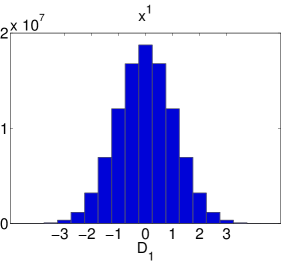
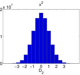
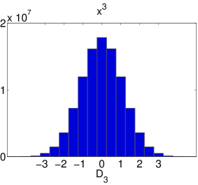
Figure 1: The distribution of normalised distances between the observation and the prior mean when the noise covariance is $R_{n}=10^{-2}\times I_{3}$.

7.2.2 $L^{2}$ norm of the higher order central moments

Here we aim to investigate the parameter regimes under which our cubature filters are likely (or unlikely) to outperform. In order to evaluate the computational error, one needs to define an error criterion relevant to the approximations. We realise that unfortunately a comparison between the evolving single trajectory and the corresponding posterior mean approximation, which is commonly used in the filtering context, is highly inappropriate for our purpose. This is because the cubature approximation is basically superior within approximating the tail behaviour or higher order moments of the probability distribution. Therefore we instead use the $L^{2}$ norm of the central moment to quantify the accuracy of the approximation obtained in the form of discrete measure.

Let $\mathcal{C}^{p}$ be the $p$-th central moment of $X=(x^{1}\;x^{2}\;x^{3})^{t}$, i.e.,

$$\mathcal{C}^{p}_{i_{1},\cdots,i_{p}}=\mathbb{E}\left(\prod_{j=1}^{p}\left(x^{i_{j}}-\mathbb{E}({x}^{i_{j}})\right)\right)$$

where $i_{j}=1,2,3$. The $L^{2}$ norm of $\mathcal{C}^{p}$ is defined by

$$\parallel\mathcal{C}^{p}\parallel_{2}\equiv\left(\sum_{i_{1},\cdots,i_{p}=1}^{3}|\mathcal{C}^{p}_{i_{1},\cdots,i_{p}}|^{2}\right)^{1/2}.$$ (7.58)

When $p=1$, Eq. (7.58) is the Euclidean norm of the vector. When $p=2$, it is equivalent with the Frobenius norm of the matrix. Let $\widehat{\mathcal{C}}^{p}$ be the $p$-th central moment of a particle approximation, then the relative root mean square error

$$\text{rmse}\%\equiv\parallel\mathcal{C}^{p}-\widehat{\mathcal{C}}^{p}\parallel_{2}/\parallel\mathcal{C}^{p}\parallel_{2}$$ (7.59)

will be calculated to measure the accuracy of the moment approximations.

7.2.3 Monte-Carlo Gaussian samples

In our problem setting, the rmse errors are insensitive to the specific time interval between successive observations. Taking one arbitrary time interval, we study the cases of $D=1,2,3$ which correspond to normal, exceptional and rare event. The scenario initially may look somewhat artificial because, unlike the filtering in practice, the observational data is not generated from realisations. However we emphasise it has been carefully designed, while keeping the practical relevance, in order to find the parameter regimes under which our approaches outperform Monte-Carlo methods and this will eventually turn out to be extremely helpful for a deeper understanding of the filtering problem.

We perform Gaussian sampling to obtain three different Monte-Carlo approximations of the posterior measure. For the first one, we draw samples from the prior measure and subsequently apply the bootstrap reweighting to obtain the posterior approximation. One can regard these bootstrap reweighted samples from the prior as SIR result. The second one is from the SISR algorithm under the transition kernel $\widetilde{K}(dx_{n}|x_{n-1},y_{n})=\mathbb{P}(dx_{n}|x_{n-1},y_{n})$, which is the optimal proposal in the sense of minimising the variance of the importance weights [14]. Finally, we draw samples directly from the posterior measures as the third one. Note, in all Monte-Carlo approximations, neither truncation error due to numerical integration nor resampling error is induced for a fair comparison. The rmse errors (7.59) of these Gaussian samples are depicted in Fig. 4 when $R=10^{-2}$, $D=1,2,3$ and in Fig. 5, when $D=1$, $R=10^{-1},10^{-2},10^{-3}$. These results will be compared with the cubature filters.

Table 1: The number of adaptive partition $k$ for KLV with $m=5$

	$\epsilon=10^{-2}$	$\epsilon=10^{-3}$	$\epsilon=10^{-4}$	$\epsilon=10^{-5}$
$R=10^{-1}$	7	31	102	344
$R=10^{-2}$	10	29	101	330
$R=10^{-3}$	20	48	120	329

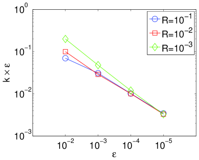
Figure 2: The upper bound of the total error along with the adaptive partition when $m=5$.

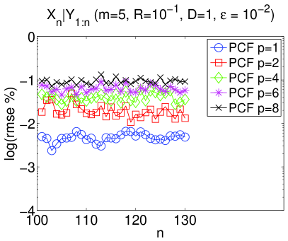
(a) PCF using adaptive partition with $\epsilon=10^{-2}$

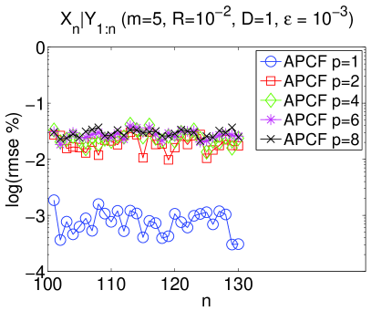
(b) APCF using adaptive partition with $\epsilon=10^{-3}$

Figure 3: The relative $L^{2}$ errors for the $p$-th moments of the evolutionary posterior.

7.3 PCF and APCF with cubature on Wiener space of degree $5$

7.3.1 Choice of parameters

We here implement the PCF and APCF at the flow level. In case of $d=3$, i.e., when the system is driven by three independent white noises, cubature on Wiener space of degree $m=3$ and $m=5$, with support size $n_{m}=6$ and $n_{m}=28$ respectively, are available. We apply the KLV operator with degree $m=5$.

Using the likelihood $g^{y_{n}}$ as the test function $f$, the adaptive partition $\mathcal{D}(\epsilon,g^{y_{n}})$ satisfying Eq. (6.52) with $\widetilde{Q}^{m}_{s_{j}}$ in place of ${Q}^{m}_{s_{j}}$ is analytically obtained for the system of Eq. (7.56). Note that the likelihood $g^{y_{n}}$ is the density function of $\mathcal{N}(y_{n},R_{n})$ and that the adaptive partition does not depend on $y_{n}$ but on $R_{n}$. The number of iterations $k$ as a function of $\epsilon$ and $R$ is listed in table 1. In this case, Fig. 2 reveals the upper bound of Eq. (6.53) tends to decrease as $\epsilon$ becomes smaller. Therefore, by choosing $\theta$ to be the same order of $\epsilon$, one can combine the adaptive partition and the adaptive recombination to achieve a desired degree of accuracy to some extent.

For the recombination of the PCF, Eq. (6.54) with $f=g^{y_{n}}$ for all $y_{n}\in\mathbb{R}^{N}$, i.e.,

$$\sup_{y_{n}}\left\lvert\left({\Phi^{m,j}_{\mathcal{D},(u,r)}}(\mu^{0})-\widehat{\Phi}^{m,j}_{\mathcal{D},(u,r)}(\mu^{0}),P_{T-t_{j}}g^{y_{n}}\right)\right\rvert<\theta$$ (7.60)

is met so that the recombination does not depend on $y_{n}$ but on $R_{n}$. We choose the recombination degree $r=5$ and simulate the PCF for the cases of $\epsilon=10^{-2},10^{-3}$ with $\theta=0.3\times\epsilon$.

For the APCF, the tolerance $\tau$ has to be chosen in addition to the parameters $\{\epsilon,\theta\}$. The value of $\tau$ varies in each case, but we choose it so that the SPL operator in Eq. (6.49) allows $1/4\sim 1/3$ part of particles leap to the next observation time for all iterations except the first and last few steps. The remaining particles are reduced by the adaptive recombination, i.e., the recombination satisfies

$$\left\lvert\left({\Phi^{m,j}_{\mathcal{D},(u,r),\tau}}(\mu^{0})-\widehat{\Phi}^{m,j}_{\mathcal{D},(u,r),\tau}(\mu^{0}),P_{T-t_{j}}g^{y_{n}}\right)\right\rvert<\theta$$ (7.61)

where $\mu^{0}=\widetilde{\pi}^{\text{APCF}}_{n-1|n-1}$. We again choose the recombination degree $r=5$ and simulate the APCF for the cases of $\epsilon=10^{-2},10^{-3}$ with $\theta=0.3\times\epsilon$.

While the value of $D$ being fixed, we apply the PCF and APCF to obtain the values of Eq. (7.59) for the evolving posterior meausre. Fig. 3 shows that the performances of the two filtering algorithms are stable and that the numerical error estimates of high order moments are insensitive to $n$ (the rest cases produce similar plots and are not shown).

In our numerical simulations, the number of patches needed to satisfy Eq. (7.60) in the PCF increases as the time partition approaches to the next observation time, eventually about $8^{3}\sim 16^{3}$. On the contrary, Eq. (7.61) in the APCF is satisfied with $2^{3}$ ($<10$) patches in most cases. As a result, APCF saves computation time significantly compared with PCF.

7.3.2 Dependence on the observation location

When $R=10^{-2}$ is fixed and $D=1,2,3$ varies, the relative $L^{2}$ errors of the $p$-th moments of PCF and APCF are shown in Figs. 4(b), 4(i), 4(j), 4(k). We have implemented two cases of $\epsilon=10^{-2}$ and $\epsilon=10^{-3}$. The recombination times are measured using Visual Studio with Intel $2.53$ GHz processor (the autonomous ODEs are solved analytically). Fig. 4 reveals the following.

• The prior approximation of PCF with $\epsilon=10^{-3}$ shows similar accuracy with $10^{4}$ Monte-Carlo sampling (Figs. 4(a), 4(b)).

• The accuracy of the APCF prior approximation is in general worse than PCF especially for higher order moments (Fig. 4(b)).

• As the observation is located further far from the prior mean, i.e., as $D$ increases, the posterior approximation obtained from Monte-Carlo bootstrap reweighting (SIR) becomes less accurate (Figs. 4(c), 4(d), 4(e)). As the number of samples $M$ increases, the error reduction asymptotically scales as $M^{-1/2}$ in all cases.

• Unlike the case of SIR, the accuracy of the importance samples (SISR) is not significantly influenced by the observation location as well as the number of samples (Figs. 4(f), 4(g), 4(h)). This sample size insensitivity is presumably because SISR duplicates the samples in this parameter regime (compare with Fig. 5(i)).

• The accuracy of the APCF posterior approximation is similar to PCF but APCF significantly reduces the recombination time which is insensitive to $D$ (Figs. 4(i), 4(j), 4(k)).

• The accuracy of the PCF and APCF posterior approximations with $\epsilon=10^{-2}$ is similar to $10^{4}$ Monte-Carlo reweighted samples (SIR) when $D=1,2$ (Figs. 4(c), 4(i), 4(d), 4(j)) and to $10^{5}$ reweighted samples (SIR) when $D=3$ (Figs. 4(e), 4(k)).

• The accuracy of the PCF and APCF posterior approximations with $\epsilon=10^{-3}$ is similar to $10^{5}$ Monte-Carlo reweighted samples when $D=1$ (Figs. 4(c), 4(i)), to $10^{6}$ reweighted samples when $D=2$ (Figs. 4(d), 4(j)) and to $10^{7}$ reweighted samples when $D=3$ (Figs. 4(e), 4(k)).

• The accuracy of the PCF and APCF posterior approximations with $\epsilon=10^{-3}$ is superior to $10^{6}$ importance samples (SISR) when $D=1$ (Figs. 4(f), 4(i)), comparable to SISR when $D=2$ (Figs. 4(g), 4(j)), inferior to SISR when $D=3$ (Figs. 4(h), 4(k)), in approximating higher order moments.

 

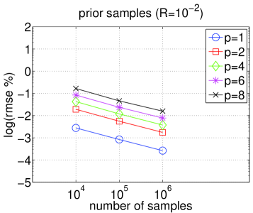
(a) unweighted prior samples

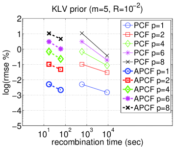
(b) cubature approximation of prior

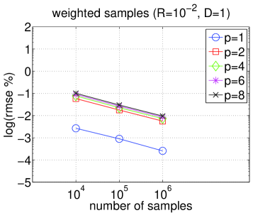
(c) bootstrap reweighted prior samples

(d) bootstrap reweighted prior samples

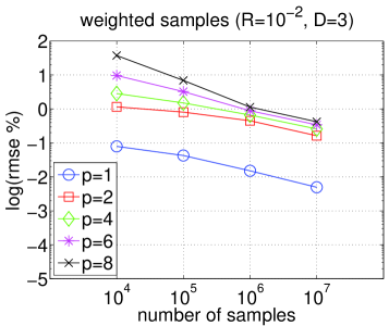
(e) bootstrap reweighted prior samples

(f) weighted posterior samples

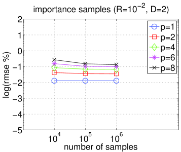
(g) weighted posterior samples

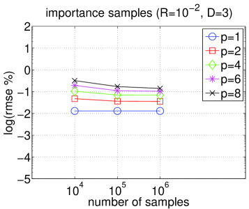
(h) weighted posterior samples

(i) cubature approximation of posterior

(j) cubature approximation of posterior

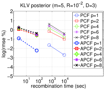
(k) cubature approximation of posterior

Figure 4: The prior and posterior approximations when $R=10^{-2}$ is fixed and $D=1,2,3$ varies. The top row is for the prior and the rest bottom three rows are for the posterior. The second row (SIR) and the third row (SISR) are from Monte-Carlo samples. The last bottom row is from cubature approximation when $\epsilon=10^{-2},10^{-3}$.

There is an important insight to be gained from this experimental analysis. Though PCF produces a more accurate description of the prior measure than APCF, the one from this naive approximation of the prior is not better at approximating the posterior. The point is that one needs an extremely accurate representation of the prior in certain localities. While APCF delivers this without undue cost, the PCF method would have to deliver this accuracy uniformly and well out into the tail of the prior. As a result, for the posterior approximation, APCF can achieve a similar accuracy with PCF but using significantly less computational cost.

In this example, the computational cost (recombination time) of PCF and APCF is uniform and irrespective of $D$ for given $\epsilon=10^{-2},10^{-3}$. However when one uses SIR to achieve the accuracy due to APCF with $\epsilon=10^{-3}$ in approximating higher order moments, one needs more computational resources (large number of particles) as $D$ becomes bigger. One also cannot expect an accuracy improvement from SISR except the rare event case ($D=3$). Therefore, in the reliability aspect, APCF is clearly advantageous over sequential Monte-Carlo methods.

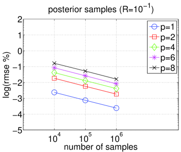
(a) unweighted posterior samples

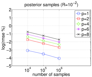
(b) unweighted posterior samples

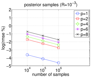
(c) unweighted posterior samples

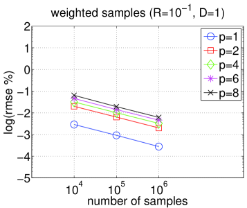
(d) bootstrap reweighted prior samples

(e) bootstrap reweighted prior samples

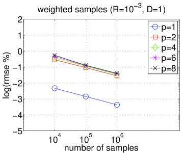
(f) bootstrap reweighted prior samples

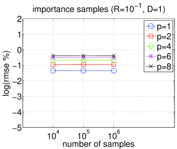
(g) weighted posterior samples

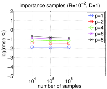
(h) weighted posterior samples

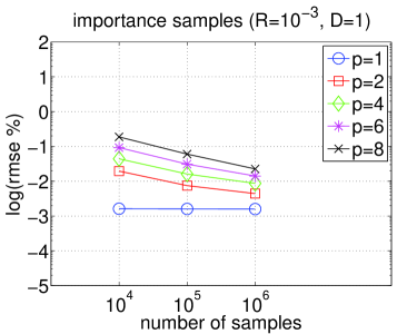
(i) weighted posterior samples

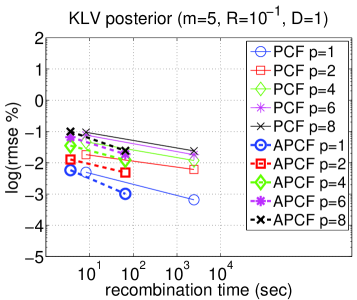
(j) cubature approximation of posterior

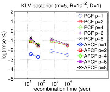
(k) cubature approximation of posterior

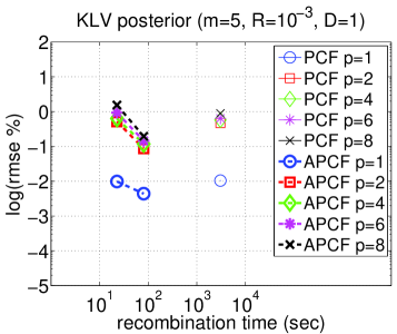
(l) cubature approximation of posterior

Figure 5: The posterior approximations when $D=1$ is fixed and $R=10^{-1},10^{-2},10^{-3}$ varies. The top three rows are from Monte-Carlo samples. The first row is from direct sampling of posterior, the second is from SIR and the third is from SISR. The last bottom row is from cubature approximation when $\epsilon=10^{-2},10^{-3}$. In Fig. 5(l), the PCF with $\epsilon=10^{-3}$ is not shown.

7.3.3 Dependence on the observation noise error

When $D=1$ is fixed and $R=10^{-1},10^{-2},10^{-3}$ varies, the values of Eq. (7.59) for PCF and APCF are shown in Figs. 5(j), 5(k), 5(l). We have implemented two cases of $\epsilon=10^{-2}$ and $\epsilon=10^{-3}$. Fig. 5 reveals the following.

• The high order moment approximations errors due to Monte-Carlo Gaussian samples (direct sampling of the posterior) are insensitive to its covariance (recall the diagonal element of $C_{n|n}$ is of the same order with the value of $R$) (Figs. 5(a), 5(b), 5(c)).

• As the likelihood becomes narrower, i.e., as $R$ decreases, the posterior approximation obtained from Monte-Carlo bootstrap reweighting (SIR) becomes less accurate (Figs. 5(d), 5(e), 5(f)).

• The accuracy of importance samples (SISR) tends to increase as $R$ decreases (Figs. 5(g), 5(h), 5(i)). In particular, when $R=10^{-3}$, the moment approximations of SISR is comparable with those from direct sampling of the posterior except the mean (Figs. 5(c), 5(i)).

• As $R$ decreases, the recombination time needed to achieve a given degree of accuracy becomes bigger for PCF but this is not the case for APCF, i.e., the recombination time for APCF is insensitive to $R$ (Figs. 5(j), 5(k), 5(l)).

The simulation shows that APCF again achieves a similar accuracy with PCF in all cases but, as the observation noise error decreases, APCF becomes more competitive than PCF for the solution of the intermittent data assimilation problem. It further shows that APCF is of higher order with respect to the recombination time and can achieve the given degree of accuracy with lower computational cost.

Although $Y_{n}$ is there and measurable it is sometimes the case that it is actually computationally very expensive to compute and that actually the thing one can compute is the evaluation of likelihood for a number of locations. For example, consider a tracking problem for an object of moderate intensity and diameter that does a random walk and is moving against a slightly noisy background and is observed relatively infrequently. Its influence is entirely local. The likelihood function will be something like the Gaussian centred at the position of object but completely uninformative elsewhere in the space. The smaller the object, the tighter or narrower the Gaussian the harder the problem of finding the object becomes. One can compute the likelihood at any point in the space, but only evaluations at the location of the particle are informative. In that way one sees that

1. The $Y_{n}$ is observable but only partially observed - and with low noise is very expensive to observe accurately as one has to find the particle.

2. The likelihood can be observed at points in the space.

In this sort of example it would be quite wrong to assume that, if we know the prior distribution of $X_{n}$ then just because $Y_{n}=X_{n}+\eta_{n}$ we know the posterior distribution at zero cost. For sequential Monte-Carlo methods, bootstrap reweighting would seem to give a much better approach.

7.4 Prospective performance PCF and APCF with cubature on Wiener space of degree $7$

A cubature formula on Wiener space of degree $m\geq 7$ is currently not available when $d=3$. However, in our problem setting, we are able to emulate a prospective performance of higher order cubature formula using Gauss-Hermite quadrature.

For the linear dynamics satisfying

$$X(\Delta)=F_{\Delta}X(0)+\nu_{\Delta},\quad\nu_{\Delta}\sim\mathcal{N}\left(0,Q_{\Delta}\right)$$

where $F_{\Delta}\in\mathbb{R}^{3\times 3}$ is a matrix, we define the forward operator

$${\text{GHC}}^{(m)}\left(\sum_{i=1}^{n}\kappa_{i}\delta_{x^{i}},\Delta\right)\equiv\sum_{i=1}^{n}\sum_{j=1}^{n_{m}}\kappa_{i}\lambda_{j}\delta_{F_{\Delta}x^{i}+z^{j}}$$ (7.62)

where $\{\lambda_{j},z^{j}\}_{j=1}^{n_{m}}$ is a Gauss-Hermite cubature of degree $m$ with respect to the law of $\nu_{\Delta}$. The authors have seen that the performance of GHC is similar to KLV on the flow level when $m=3,5$ and that Eq. (7.62) can be used as an alternative to Eq. (4.30) in the application of PCF and APCF to the test model.

Table 2: The number of adaptive partition $k$ for GHC with $m=7$

	$\epsilon=10^{-2}$	$\epsilon=10^{-3}$	$\epsilon=10^{-4}$	$\epsilon=10^{-5}$
$R=10^{-1}$	2	4	6	10
$R=10^{-2}$	5	9	16	28
$R=10^{-3}$	9	17	30	54

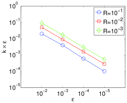
Figure 6: The upper bound of the total error along with the adaptive partition when $m=7$.

The number of iterations $k$ in the adaptive partition, obtained from using GHC with Gauss-Hermite cubature of degree $m=7$ whose support size is $n_{m}=64$ in place of $Q^{m}_{s_{j}}$, is shown in table 2. Here Fig. 6 corresponds to Fig. 2 and shows an enhanced accuracy. We apply GHC with degree $m=7$ to obtain a prior and posterior approximation, where the recombination degree $r=5$ and $\theta=0.2\times\epsilon$ is used. Our choice of $\tau$ is again such that $1/4\sim 1/3$ of the particles are allowed to leap to the next observation time. The rmse errors (7.59) in the case of $R=10^{-2}$, $D=2$ and $\epsilon=10^{-2},10^{-3}$ are shown in Fig. 7(c) and this can be viewed as a result from PCF and APCF with cubature on Wiener space of degree $m=7$. Its performance is in fact one higher order improvement for both accuracy and recombination time in view of Figs. 7(a), 7(b). From the simulation, we expect APCF with higher order cubature formula can outperform Monte-Carlo approximations in any parameter regimes including the ones for which it used to be not so successful when it uses a low order cubature formula. This further highlights the strong necessity to find out cubature formula on Wiener space of degree $m\geq 7$ in order to solve the PDE or filtering problem with high accuracy in a moderate dimension.

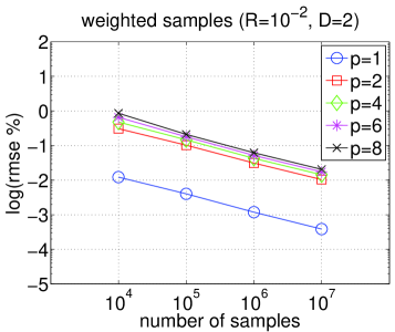
(a) bootstrap reweighted prior samples

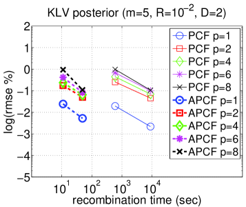
(b) cubature approximation of posterior

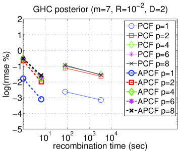
(c) cubature approximation of posterior

Figure 7: The posterior approximations when $R=10^{-2}$ and $D=2$. The left is from Monte-Carlo samples and the middle and right is from cubature approximation when $\epsilon=10^{-2},10^{-3}$.

8 Discussion

In this paper we introduce a hybrid methodology for the numerical resolution of the filtering problem which we named the adaptive patched cubature filter (APCF). We explore some of its properties and we report on a first attempt at a practical implementation. The APCF combines many different methods, each of which addresses a different part of the problem and has independent interest. At a fundamental level all of the methods use high order approaches to quantify uncertainty (cubature), and also to reduce the complexity of calculations (recombination based on heavy numerical linear algebra), while retaining explicit thresholds for accuracy in the individual computation. The thresholds for accuracy in a stage are normally achievable in a number of ways (e.g., small time step with low order, or large time step with high order) and the determination of these choices depends on computational cost. Aside from this use of the error threshold and choices based on computational efficiency there are several other points to observe in our development of this filter.

1. One feature is the surprising ease with which one can adapt the computations to the observational data and so avoid performing unnecessary computations. In even moderate dimensions (we work in $3+1$) this has a huge impact for the computation time while preserving the accuracy we achieve for the posterior distribution (Figs. 4(i), 4(j), 4(k), Figs. 5(j), 5(k), 5(l)). It is an automated form of deterministic high order importance sampling which has wider application than the one explored in this paper, for instance it is used to deliver accurate answers to PDE problems with piecewise smooth test function in the example developed in [29].

2. Another innovation allowing a huge reduction in computation is the ability to efficiently patch the particles in the multiple dimensional scenario. Although the problem might at first glance seem elementary, it is in fact the problem of data classification. To resolve this problem we introduce an efficient algorithm for data classification based on extending the Morton order to floating point context. This method has now also been used effectively for efficient function extrapolation [34].

3. The KLV algorithm is at the heart of a number of successful methods for solving PDEs in moderate dimension [33]. In each case, something has to be done about the explosion of scenarios after each time step; this in turn has to rely on and understanding the errors. In this paper we take a somewhat different approach to the literature [31] in the way we use higher order Lipschitz norms systematically to understand how well functions have been smoothed, and to measure the scales on which they can be well approximated by polynomials. This has the consequence that one can be quite precise about the errors one incurs at each stage in the calculation. In the end this is actually quite crucial to the logic of our approach since an efficient method requires optimisation over several parameters - something that is only meaningful if there are (at least in principle) uniform estimates on errors. As a result of this perspective, we do not follow the time steps and analytic estimates introduced by Kusuoka in [26] although we remain deeply influenced by balancing the smoothing properties of the semigroup with the use of non-equidistant time steps.

4. The focus on Lipschitz norms makes it natural to apply an adaptive approach to the recombination patches as well as to the prediction process. In both cases we can be lead by the local smoothness of the likelihood function as sampled on our high order high accuracy set of scenarios.

5. We have focussed our attention on the quality of the tail distribution of the approximate posterior we construct. This is important in the filtering problem because a failure to describe the tail behaviour of the tracked object implies that one will lose the trajectory all together at some point. These issues are particularly relevant in high dimensions as the cost of increasing the frequency of observation can be prohibitive. If one wishes to ensure reliability of the filter in the setting where there is a significant discrepancy between the prior estimate and the realised outcome over a time step then our APCF with cubature on Wiener space of degree $5$ already shows in the three dimensional example that it can completely outperform sequential importance resampling Monte-Carlo approach. The absence, at the current time, of higher order cubature formulae is in this sense very frustrating as the evidence we give suggests that higher degree methods will lead to substantial further benefits for both computation and accuracy.

In putting this paper together we have realised that there are many branches in this algorithm that can be improved, in particular some parts of the adaptive process and also the recombination (a theoretical improvement in the order of recombination has recently been discovered [38]). There are also large parts that can clearly be parallelised. We believe that there is ongoing scope for increasing the performance of the APCF.

References

- [1] B. Anderson and J. Moore, Optimal filtering, vol. 11, Prentice-hall Englewood Cliffs, NJ, 1979.
- [2] V. Beneš, Exact finite-dimensional filters for certain diffusions with nonlinear drift, Stochastics: An International Journal of Probability and Stochastic Processes, 5 (1981), pp. 65–92.
- [3] R. R. Bitmead and M. Gevers, Riccati difference and differential equations: Convergence, monotonicity and stability, The Riccati Equation, (1991), pp. 263–291.
- [4] J. Carpenter, P. Clifford, and P. Fearnhead, Improved particle filter for nonlinear problems, in Radar, Sonar and Navigation, IEE Proceedings-, vol. 146, IET, 1999, pp. 2–7.
- [5] D. Crisan and A. Doucet, A survey of convergence results on particle filtering methods for practitioners, Signal Processing, IEEE Transactions on, 50 (2002), pp. 736–746.
- [6] D. Crisan and S. Ghazali, On the convergence rates of a general class of weak approximations of sdes, Stochastic differential equations: theory and applications, 2 (2006), pp. 221–248.
- [7] D. Crisan and T. Lyons, Minimal entropy approximations and optimal algorithms for the filtering problem, Monte Carlo methods and applications, 8 (2002), pp. 343–356.
- [8] D. Crisan and S. Ortiz-Latorre, A kusuoka–lyons–victoir particle filter, Proceedings of the Royal Society A: Mathematical, Physical and Engineering Science, 469 (2013), p. 20130076.
- [9] D. Crisan and B. Rozovskii, The Oxford handbook of nonlinear filtering, Oxford University Press, 2011.
- [10] P. Del Moral, Mean field simulation for monte carlo integration chapman & hall: London, (2013).
- [11] P. Del Moral and F.-K. Formulae, genealogical and interacting particle systems with applications, probability and its applications, 2004.
- [12] A. Doucet, N. De Freitas, and N. Gordon, Sequential Monte Carlo methods in practice, Springer Verlag, 2001.
- [13] A. Doucet, S. Godsill, and C. Andrieu, On sequential monte carlo sampling methods for bayesian filtering, Statistics and computing, 10 (2000), pp. 197–208.
- [14] A. Doucet and A. M. Johansen, A tutorial on particle filtering and smoothing: Fifteen years later, Handbook of Nonlinear Filtering, 12 (2009), pp. 656–704.
- [15] G. Evensen, Data assimilation: the ensemble Kalman filter, Springer Verlag, 2009.
- [16] A. Gelb, Applied optimal estimation, MIT press, 1974.
- [17] N. Gordon, D. Salmond, and A. Smith, Novel approach to nonlinear/non-gaussian bayesian state estimation, in Radar and Signal Processing, IEE Proceedings F, vol. 140, IET, 1993, pp. 107–113.
- [18] L. Gyurkó and T. Lyons, Efficient and practical implementations of cubature on wiener space, Stochastic Analysis 2010, (2011), pp. 73–111.
- [19] A. Jazwinski, Stochastic processes and filtering theory, vol. 64. san diego, california: Mathematics in science and engineering, 1970.
- [20] R. Kalman et al., A new approach to linear filtering and prediction problems, Journal of basic Engineering, 82 (1960), pp. 35–45.
- [21] R. E. Kalman and R. S. Bucy, New results in linear filtering and prediction theory, Journal of Basic Engineering, 83 (1961), pp. 95–108.
- [22] P. Kloeden and E. Platen, Numerical solution of stochastic differential equations, vol. 23, Springer, 2011.
- [23] H. Kushner, Approximations to optimal nonlinear filters, Automatic Control, IEEE Transactions on, 12 (1967), pp. 546–556.
- [24] S. Kusuoka, Approximation of expectation of diffusion process and mathematical finance, Advanced Studies in Pure Mathematics, 31 (2001), pp. 147–165.
- [25] , Malliavin calculus revisited, J. Math. Sci. Univ. Tokyo, 10 (2003), pp. 261–277.
- [26] S. Kusuoka, Approximation of expectation of diffusion processes based on lie algebra and malliavin calculus, in Advances in mathematical economics, Springer, 2004, pp. 69–83.
- [27] S. Kusuoka and D. Stroock, Applications of the malliavin calculus. iii, (1987).
- [28] C. Litterer and T. Lyons, Introducing cubature to filtering. In Crisan, Dan and Rozovskii, Boris [9], pages 768-796.
- [29] , High order recombination and an application to cubature on wiener space, The Annals of Applied Probability, 22 (2012), pp. 1301–1327.
- [30] J. S. Liu and R. Chen, Sequential monte carlo methods for dynamic systems, Journal of the American statistical association, 93 (1998), pp. 1032–1044.
- [31] T. Lyons and N. Victoir, Cubature on wiener space, Proceedings of the Royal Society of London. Series A: Mathematical, Physical and Engineering Sciences, 460 (2004), pp. 169–198.
- [32] G. M. Morton, A computer oriented geodetic data base and a new technique in file sequencing, International Business Machines Company, 1966.
- [33] S. Ninomiya and N. Victoir, Weak approximation of stochastic differential equations and application to derivative pricing, Applied Mathematical Finance, 15 (2008), pp. 107–121.
- [34] W. Pan, Cubature and tarn option pricing. unpublished.
- [35] M. K. Pitt and N. Shephard, Filtering via simulation: Auxiliary particle filters, Journal of the American statistical association, 94 (1999), pp. 590–599.
- [36] M. Putinar, A note on tchakaloff’s theorem, Proceedings of the American Mathematical Society, 125 (1997), pp. 2409–2414.
- [37] C. Reutenauer, Free lie algebras, Handbook of algebra, 3 (2003), pp. 887–903.
- [38] M. Tchernychova. private communication.
- [39] G. Uhlenbeck and L. Ornstein, On the theory of the brownian motion, Physical Review, 36 (1930), p. 823.
- [40] P. van Leeuwen, Nonlinear data assimilation in geosciences: an extremely efficient particle filter, Quarterly Journal of the Royal Meteorological Society, 136 (2010), pp. 1991–1999.
- [41] N. Watanabe and N. Ikeda, Stochastic differential equations and diffusion processes, North Holland Math. Library/Kodansha, Amsterdam/Tokyo, (1981).