A Total Fractional-Order Variation Model for Image Restoration with Non-homogeneous Boundary Conditions and its Numerical Solution

Abstract

To overcome the weakness of a total variation based model for image restoration, various high order (typically second order) regularization models have been proposed and studied recently. In this paper we analyze and test a fractional-order derivative based total $\alpha$-order variation model, which can outperform the currently popular high order regularization models. There exist several previous works using total $\alpha$-order variations for image restoration; however first no analysis is done yet and second all tested formulations, differing from each other, utilize the zero Dirichlet boundary conditions which are not realistic (while non-zero boundary conditions violate definitions of fractional-order derivatives).

This paper first reviews some results of fractional-order derivatives and then analyzes the theoretical properties of the proposed total $\alpha$-order variational model rigourously. It then develops four algorithms for solving the variational problem, one based on the variational Split-Bregman idea and three based on direct solution of the discretise-optimization problem. Numerical experiments show that, in terms of restoration quality and solution efficiency, the proposed model can produce highly competitive results, for smooth images, to two established high order models: the mean curvature and the total generalized variation.

Keywords. Fractional-order derivatives; Total $\alpha$-order variation; PDE; Image Denoising; Image inverse problems; Optimization methods.   AMS. 62H35, 65N22, 65N55, 74G65, 74G75

1 Introduction

This paper presents a fractional-order derivative based regularizer for variational image restoration. It may be used for other imaging models such as image registration. Denote an observed image by $z=z(x)$, $x\in\Omega\subset\mathbb{R}^{d}$ where $\Omega$ is the bounded domain of the image with $d$ space dimension and has a Lipschitz boundary. Here we consider $d=2$ and mainly the image denoising problem with an additive noise i.e. assume $z=u+\eta_{0}$ with $\eta_{0}$ representing some unknown Gaussian noise of mean zero and deviation $\sigma$, but most results are applicable to $d>2$ and other noise models.

1.1 Image inverse problem

Restoring the unknown $u$ (without any restrictions) from $z$ is an inverse problem. According to the maximum likelihood principle [39], most image processing problems involve solving the least-square problem

$$\min_{u}\int_{\Omega}|P(u)-z|^{2}dx,$$ (1)

measuring the fidelity to $z$. For example, $P(u)=u$ for image denoising, $P(u)$ takes the template image $T(x+u(x))$ (and $z=R(x)$ for a reference image) for image registration, and $P(u)=P_{\Omega_{1}}(u(x))$ for image inpainting with $\Omega_{1}\subset\Omega$ the subdomain with missing data.

The problem (1) is in general ill-posed due to non-uniqueness, therefore how to effectively solve it becomes a fundamental task in image sciences. The most popular idea is to regularize it so that the resulting well-posed problem admits an unique solution. The classical regularization technique by Tikhonov et. al [76] is to add a smoothing regularization term into the energy functional to derive the following minimization problem

$$\min_{u}\int_{\Omega}|P(u)-z|^{2}dx+\lambda\int_{\Omega}|\nabla u|^{2}dx,$$ (2)

where $\lambda$ is a positive constant. This model cannot preserve image edges, though it is simple to use. The total variation (TV) model by Rudin-Osher-Fatemi [67] or the ROF model

$$\min_{u}\int_{\Omega}|\nabla u|dx,\qquad\int_{\Omega}|P(u)-z|^{2}dx=\sigma^{2},\ \ P(u)=u$$ (3)

is widely used, where $\sigma$ is an estimate of the error $\eta_{0}$ between the noisy image $z$ and the true data $u$. The ROF model preserves the image edges by seeking solutions of piecewise constant functions in the space of bounded variation functions (BV). A variety of methods based on the TV regularization have been developed to deal with the imaging problems such as image restoration [1, 2, 10, 82], image registration [48, 37, 62], image decomposition [61, 38, 32], image inpainting [46, 40, 41, 24] and image segmentation [16, 77]. Restoring smooth images in some applications where edges are not the main features presents difficulties for the ROF model as it can yield the so-called blocky (staircase) effects. Another disadvantage of the model is to the loss of image contrasts [52]. It should be remarked that the recently popular method by the iterative regularization technique [60] can reduce the staircasing effect and improve on the image contrast to some extent; besides it provides a fast implementation.

1.2 High-order regularization

To remedy the above mentioned two drawbacks (stairicasing and contrast), two types of alternative regularizer to the TV have been proposed in the literature. The first type introduces higher order regularization into image variational models [22, 72, 7, 52, 74, 31, 15, 84]. The mean curvature-based variation denoising model was studied in [52, 53, 17, 84] where the regularized solution $u$ is obtained by solving the fourth-order Euler-Lagrangian equation. Bredies et al. [15] proposed the total generalized variation regularizer involving a linear combination of higher-order derivatives and the TV of $u$ to model the image denoising while Chang et al. [25] considered a nonlinear combination of regularizer based on first and second order derivatives. For image inpainting, a high order regularization based on Euler’s elastica of $u$ is used in [72]. Similarly the Euler’s elastica energy [56] and mean curvature [36, 29] are also proposed to transform the template image $T(x+u)$ to map the reference image $R(x)$ in image registration; see also [35, 51]. The above mentioned high order regularization methods are effective but due to high nonlinearity efficient numerical solution is a major issue.

The second type introduces fractional-order derivatives, which are widely studied in other research subjects beyond image processing [3, 5, 6, 8, 85], into regularization of images. For example, Bai and Feng [11] introduced first fractional-order derivative into anisotropic diffusion equations for noise removal

$$\frac{\partial u}{\partial t}=-D^{\alpha*}_{x}(c(|D^{\alpha}u|)D^{\alpha}u)-D^{\alpha*}_{y}(c(|D^{\alpha}u|)D^{\alpha}u),$$ (4)

where $c(\cdot)$ denotes the divergence parameter and $D_{x}^{\alpha*}$ denotes the adjoint operator of $D_{x}^{\alpha}$, which may be viewed as a generalization of the Perona-Malik model. Although the above equation can be related to the Euler-Lagrange equations of an energy functional with the fractional derivative of the image intensity, generalizing commonly used PDE models, the energy minimization models are not studied as such. The discrete Fourier transform is used to implement the numerical algorithm assuming a periodic input image at its borders [11]. See also [45, 44, 49, 66] for more motivations and studies based on the above diffusion equation. Chen et al. [28, 27, 26] considered the fractional-order TV-$L^{2}$ image denoising model

$$\min\limits_{u}\Big{\{}E(u):=\int_{\Omega}\sqrt{(D^{\alpha}_{x}u)^{2}+(D^{\alpha}_{y}u)^{2}}d\Omega+\frac{\lambda}{2}\|u-f\|^{2}_{2}\Big{\}}$$ (5)

and numerically obtained improved denoising results over the Perona-Malik and ROF models; however no analysis was given. There, they converted this primal formulation into a dual problem for the new dual variable ${\mathbf{p}}=(p_{1},p_{2})$ by $u=f-\mbox{div}^{\alpha}{\mathbf{p}}/\lambda$ and used a dual algorithm using the gradient descent idea similar to the Chambolle method [18] for the ROF. In [81], the authors proposed a discrete optimization framework for image denoising problem where the fractional order derivative is used to model the regularization term,

$$\min_{u}\Big{\{}\sum_{i,j=1}^{N}|(\nabla^{\alpha}u)_{i,j}|+1/2\sum_{j=0}^{L}2^{-2js_{j}}|[\lambda(f-u)_{j}]|^{2},\;1\leq\alpha\leq 2,0\leq s_{j}\leq 1\Big{\}},$$ (6)

which is solved by an alternating projection algorithm. See also [21].

These works have reflected good performance of the fractional order derivative in achieving a satisfactory compromise such as no stair-casing and in preserving important fine-scale features such as edges and textures. These encouraging results motivated us to investigate this new model more closely.

There have been several other works involving discrete forms of an $\alpha$-order derivative proposed to tackle image registration problem [78, 54] and image inpainting problem [83]. Comparing with the first type of high order models [15, 36, 29], a fractional order model (type two) is less nonlinear and hence is more amenable to developing fast iterative solvers. Clearly there is strong evidence to suggest that fractional order derivatives may be effective regularizer for imaging applications. There is an urgent need to establish a rigorous theory for the total $\alpha$-order variation based variational model so that further applications to image inverse problems can be considered in a systematic way.

1.3 Our contributions

This work is substantially different from previous studies. We mainly focus on the continuous total $\alpha$ variation-based model, instead of discrete formulation, and its analysis and associated numerical algorithms.

Our contributions are four-fold:

• We analyze properties of the total $\alpha$-order variation laying foundations for applications to image inverse problems as a regulariser;

• We give a new method for treating non-zero Dirichlet boundary conditions which represents a generalization of similar results that existed only in 1D to 2D;

• We establish the convexity, the solvability and a solution theory for the total $\alpha$-order variation model to make it more advantageous to work with than high order and non-convex counterparts (such as a mean curvature based model) which are not gradient based and do not have much known theory on their solutions;

• We propose and test four solution algorithms (respectively Split-Bregman based, forward-backward algorithm, Nesterov accelerated method and fast iterative shrinkage-thresholding algorithm – FISTA) to solve the underlying total $\alpha$-order variation model. We also compare with related models.

Our work is hoped to motivate further studies and facilitate future applications of $\alpha$-order variation based regularizer to other imaging problems in the community.

The rest of the paper is organized as follows. Section 2 reviews the definitions and basic properties of the fractional order derivative. Section 3 first defines the total $\alpha$-order variation and the space of functions of fractional-order bounded variations. In this space, it then analyzes the the existence and the uniqueness of the solution of the total $\alpha$-order variation based model for denoising. In Section 4, a boundary condition regularization method for treating nonzero Dirichlet boundary conditions is proposed to effectively employ and compute the fractional order derivatives of an image. Section 5 first discusses the discretization of the fractional order derivatives by a finite difference method and presents a Split-Bregman scheme for effective solution. Section 6 takes the alternative discretise-optimize solution approach and develops three optimization-based algorithms (Forward-backward algorithm, Nesterov accelerated method and FISTA) to solve the image denoising model. Experimental results are shown in Section 7, and the paper is concluded with a summary in Section 8.

2 Review of fractional-order derivatives

This section reviews definitions and simple properties of a fractional order derivative which has a long history and may be considered as a generalization of the integer order derivatives. Three popular definitions to be reviewed are the Riemann-Liouville (R-L), the Grünwald-Letnikov (G-L) and the Caputo definitions [55, 59, 63].

In this paper, a fraction $\alpha\in{\mathbb{R}}^{+}$ is assumed to lie in between two integers $n-1,n$ i.e. $0\leq\ell=n-1<\alpha<n$ and a fractional $\alpha$-order differentiation at point $x\in{\mathbb{R}}$ is denoted by the differential operator $D_{[a,x]}^{\alpha}$, where $a$ and $x$ are the bounds of the integral over a 1D computational domain. Undoubtedly, the gamma function is very important for the study of fractional derivative, which is defined by the integral [63]

$$\Gamma(z)=\int_{0}^{\infty}e^{-t}t^{z-1}\;dt.$$

One of the basic properties is that $\Gamma(z+1)=z\Gamma(z)$ and hence $\Gamma(n)=n!$. Before introducing formal definitions, we review the following informative but classical example:

Example 1

The Abel’s integral equation, with,

$$\frac{1}{\Gamma(\alpha)}\int_{0}^{x}\frac{\psi(\tau)}{(x-\tau)^{1-\alpha}}d\tau=f(x),\quad x>0$$ (7)

has the solution given by the well-known formula

$$\psi(x)=\frac{1}{\Gamma(1-\alpha)}\frac{d}{dx}\int_{0}^{x}\frac{f(\tau)}{(x-\tau)^{\alpha}}d\tau,\quad x>0.$$ (8)

This example helps to understand the formal definitions of fractional derivatives. In fact for $0<\alpha<1$, equation (7) taking on the form $I^{\alpha}_{[0,x]}\psi(x):=D^{-\alpha}_{[0,x]}\psi(x)=f(x)$ is called the fractional $\alpha$-order left R-L integral of $\psi(x)$, and equation (8) taking on the form $D^{\alpha}_{[0,x]}f(x)=\psi(x)$ is defined as the fractional $\alpha$-order left R-L derivative of $f(x)$. As operators, under suitable conditions [68], we have $D^{-\alpha}_{[0,x]}D^{\alpha}_{[0,x]}=I$ where $I$ denotes the identity operator.

The first definition of a general order $\alpha$ derivative is the left sided R-L derivative

$$D^{\alpha}_{[a,x]}f(x)=\frac{1}{\Gamma(n-\alpha)}\left(\frac{d}{dx}\right)^{n}\int^{x}_{a}\frac{f(\tau)d\tau}{(x-\tau)^{\alpha-n+1}}.$$ (9)

Subsequently the right-sided R-L and the Riesz-R-L (central) fractional derivative are respectively given by

$$\qquad D^{\alpha}_{[x,b]}f(x)=\frac{(-1)^{n}}{\Gamma(n-\alpha)}\left(\frac{d}{dx}\right)^{n}\int^{b}_{x}\frac{f(\tau)d\tau}{(\tau-x)^{\alpha-n+1}}$$

and

$$D^{\alpha}_{[a,b]}f(x)=\frac{1}{2}\left(D^{\alpha}_{[a,x]}f(x)+(-1)^{n}D^{\alpha}_{[x,b]}f(x)\right).$$

The second definition is the G-L left-sided derivative denoted by

$${}^{G}D^{\alpha}_{[a,x]}f(x)=\lim\limits_{h\rightarrow 0}\frac{1}{h^{\alpha}}\sum_{j=0}^{[\frac{x-a}{h}]}(-1)^{j}\Bigg{(}\begin{array}[]{c}\alpha\\ j\\ \end{array}\Bigg{)}f(x-jh),\;\;\;\Bigg{(}\begin{array}[]{c}\alpha\\ j\\ \end{array}\Bigg{)}=\frac{\alpha(\alpha-1)\dots(\alpha-j+1)}{j!},$$ (10)

which resembles the definition for an integer order derivative, where $[\vartheta]$ is the integer such that $\vartheta-1<[\vartheta]\leq\vartheta$. The third definition is the Caputo order $\alpha$ derivative defined by

$${}^{C}D^{\alpha}_{[a,x]}f(x)=\frac{1}{\Gamma(n-\alpha)}\int^{x}_{a}\frac{f^{(n)}(\tau)d\tau}{(x-\tau)^{\alpha-n+1}}.$$ (11)

where $f^{(n)}$ denotes the $n^{th}$-order derivative of function $f(x)$. The right sided derivative and the Riesz-Caputo fractional derivative are similarly defined by

$${}^{C}D^{\alpha}_{[x,b]}f(x)=\frac{(-1)^{n}}{\Gamma(n-\alpha)}\int^{b}_{x}\frac{f^{(n)}(\tau)d\tau}{(\tau-x)^{\alpha-n+1}},\quad{}^{C}D^{\alpha}_{[a,b]}f(x)=\frac{1}{2}\left({}^{C}D^{\alpha}_{[a,x]}f(x)+(-1)^{n}{}^{C}D^{\alpha}_{[x,b]}f(x)\right).$$

When $\alpha=n-1$ is an integer, the above left-sided R-L definition reduces to the usual definition for a derivative. One notes that when a function is $n-1$ times continuously differentiable and its $n$th derivative is integrable, the fractional derivatives by the above definitions are equivalent subject to homogeneous boundary conditions [63]. However we do not require such equivalence for our image function $u$; refer to Remark 2 later.

Fractional derivatives have many interesting properties — below we review a few that are useful to this work.

Linearity. For a fractional derivative $D^{\alpha}_{[a,x]}$ by any of the above three definitions, then one has

$$D^{\alpha}_{[a,x]}(p\;f(x)+q\;g(x))=p\;D^{\alpha}_{[a,x]}f(x)+q\;D^{\alpha}_{[a,x]}g(x),$$

for any fractional differentiable functions $f(x),g(x)$ and $p,q\in\mathbb{R}$. This property will be shortly used to prove convexity and to derive the first order optimal conditions.

Zero fractional derivatives. An integer derivative of an image $u$ at pixels of flat regions may be close to zero but the left R-L derivative of a constant intensity function is not zero. One advantage of minimizing a R-L derivative instead of the total variation (image gradients) could be a non-constant solution. It would be interesting to know the kind of functions that have zero $\alpha$-order derivatives.

Lemma 1 (Singularity)

Assume that $D^{\alpha}_{[a,x]}$ is one of the above three fractional-order derivative operators. For any non-integer $\alpha>0$ and $x>a$, there exists a non-constant value function $f(\tau)$ in $(a,x]$ such that $D^{\alpha}_{[a,x]}f(x)=0.$

• We give explicit constructions. Here we only consider the R-L and Caputo derivatives; for G-L derivative, we can derive a similar conclusion through their equivalency.

  1. Assume that $0<\alpha<1$, for some $x>0$, if $f(\tau)$ is taken as

     $$f(\tau)=(x-2\tau)(x-\tau)^{\alpha}$$

     for any $\tau\in(0,x]$ in Abel’s inverse transform (8), then $D^{\alpha}_{[0,x]}f(x)=\psi(x)=0$;

  2. Assume that $\alpha>1$, if $f(\tau)$ is taken as

     $$f(\tau)=(x-\tau)^{\alpha-1}$$

     for any $\tau\in(a,x]$ in $\alpha$-order R-L derivative, then $D^{\alpha}_{[a,x]}f(x)=0$;

  3. Assume that $\alpha>0$ in Caputo derivative definition, if $f(\tau)$ is taken as

     $$f(\tau)=(x-\tau)^{n-1}$$

     for any $\tau\in(a,x]$ in equation (11), then ${}^{C}D^{\alpha}_{[a,x]}f(x)=0.$

  Actually for any $\alpha>0$, the left R-L $D_{[0,x]}^{\alpha}f(x)=0$ if $f(x)=x^{\alpha-k}$ for all $k=1,2,\dots,1+\ell$ (note $\ell=[\alpha]=n-1$); refer to [47].

Remark 1

For our later applications §7, we take $1<\alpha<2$. Hence we have the left R-L $D_{[0,x]}^{\alpha}f(x)=0$ if $f(x)=x^{\alpha-1}$ or $x^{\alpha-2}$ i.e. $f(x)=x^{0.6}$ or $x^{-0.4}$ when $\alpha=1.6$. For the Caputo derivative, ${}^{C}D_{[0,x]}^{\alpha}f(x)=0$ if $f(x)=1$ or $x$.

Boundary conditions. For the left R-L derivative $D^{\alpha}_{[a,x]}f(x)$ of $f(x)$, one assumes that $f(a)=0$ or $f(b)=0$ for the right R-L derivative; otherwise there is a singularity at the end point. So the Riesz R-L derivative would require $f(a)=f(b)=0$. One solution for nonzero Dirichlet boundary conditions for $f$ would be to extract off a linear approximation $g(x)$ (that coincides with $f$ at $x=a,b$) and to consider $D^{\alpha}_{[a,x]}(f(x)-g(x))$; however there was no such a method for the 2D case. In Jumarie’s work [50], a simple alternative is to modify the R-L derivative to the following

$$D^{\alpha}_{[a,x]}f(x)=\frac{1}{\Gamma(n-\alpha)}\left(\frac{d}{dx}\right)^{n}\int^{x}_{a}\frac{f(\tau)-f(a)}{(x-\tau)^{\alpha-n+1}}d\tau,$$

also ensuring that the new fractional derivative of a constant is equal to zero and removing the singularity at $x=a$ [8]. In Section 4, we present one method for treating nonzero Dirichlet boundary conditions in 2D.

3 The total $\alpha$-order variation and its related model

This section first studies the properties of the total $\alpha$-order variation, second analyzes a total $\alpha$-order variation based denoising model and finally presents a numerical algorithm. For the classical total variation based model, its solution lies in a suitable space called the function space $\text{BV}(\Omega)$ of bounded variation [23, 69, 15]. From tests, the total fractional-order variation model can preserve both edges and smoothness of an image; we anticipate from the former that its solution should lie in a space similar to the BV space and from the latter that the smoothness is due to the non-local nature of the new regulariser.

It turns out that for total $\alpha$-order variation using $\alpha$-order derivatives, a suitable space is the space $\text{BV}^{\alpha}(\Omega)$ of functions of $\alpha$-bounded variation on $\Omega$ which will be defined and studied next. The work of this section is motivated by analysis of the total variation (TV) [1, 9, 18] and of the total generalized variation (TGV) [15].

In variational regularization methods, integration by parts involves the space of test functions in addition to the main solution space. Before discussing the total $\alpha$-order variation, we give the following definition:

Definition 1 (A space of test functions)

Let $\mathcal{C}^{\ell}(\Omega,\mathbb{R}^{d})$ denote the space of $\ell$-order continuously differentiable functions. Furthermore for any $\mathcal{C}^{\ell}(\Omega,\mathbb{R}^{d})\ni v:\Omega\mapsto\mathbb{R}^{d}$, if the $(\ell+1){th}$ order derivative $v^{(\ell+1)}$ is integrable and $\frac{\partial^{i}v(x)}{\partial n^{i}}|_{\partial\Omega}=0$ for all $i=0,1,\dots,\ell$, $v$ is compactly supported continuous-integrable function in $\Omega$. Therefore the $\ell$-compactly supported continuous-integrable function space is denoted by $\mathscr{C}_{0}^{\ell}(\Omega,\mathbb{R}^{d})$.

Definition 2 (Total $\alpha$-order variation)

Let $K$ denote the space of special test functions

$$\begin{split}K:=\Big{\{}\boldsymbol{\phi}\in\mathscr{C}_{0}^{\ell}(\Omega,\mathbb{R}^{d})\;\Big{|}\;|\boldsymbol{\phi}(x)|\leq 1\;\text{for all}\;x\in\Omega\Big{\}}\end{split}$$

where $|\boldsymbol{\phi}|=\sqrt{\sum_{i=1}^{d}\phi_{i}^{2}}$. Then the total $\alpha$-order variation of $u$ is defined by

$$\text{TV}^{\alpha}(u):=\sup\limits_{\boldsymbol{\phi}\in K}\int_{\Omega}\Big{(}-u\;\text{div}^{\alpha}\;\boldsymbol{\phi}\Big{)}dx,$$

where $\text{div}^{\alpha}\boldsymbol{\phi}=\sum_{i=1}^{d}\frac{\partial^{\alpha}\phi_{i}}{\partial x_{i}^{\alpha}}$ and $\frac{\partial^{\alpha}\phi_{i}}{\partial x_{i}^{\alpha}}$ denotes a fractional $\alpha$-order derivative $D^{\alpha}_{[a,b]}\phi_{i}$ of $\phi_{i}$ along $x_{i}$ direction.

We note that $\text{TV}^{\alpha}(u)$ is the same for any definition of $\frac{\partial^{\alpha}\phi_{i}}{\partial x_{i}^{\alpha}}$ because $\boldsymbol{\phi}$ satisfies the equivalence conditions. However for our applications in the paper, $\frac{\partial^{\alpha}u}{\partial x_{i}^{\alpha}}$ is generally not the same for different fractional derivatives (not even in the distributional sense).

Based on the $\alpha$-BV semi-norm, the $\alpha$-BV norm is defined by

$$\|u\|_{\text{BV}^{\alpha}}=\|u\|_{L^{1}}+\text{TV}^{\alpha}(u),$$ (12)

and further the space of functions of $\alpha$-bounded variation on $\Omega$ can be defined by

$$\text{BV}^{\alpha}(\Omega):=\Big{\{}u\in L^{1}(\Omega)\ \ \big{|}\ \ \text{TV}^{\alpha}(u)<+\infty\Big{\}}.$$ (13)

Lemma 2 (Lower semi-continuity)

Let $\{u^{k}(x)\}$ be a sequence from $\text{BV}^{\alpha}(\Omega)$ which converge in $L^{1}(\Omega)$ to a function $u(x)$. Then $\text{TV}^{\alpha}(u)\leq\liminf\limits_{k\rightarrow\infty}\text{TV}^{\alpha}(u^{k}).$

• Since $\ u_{k}\in BV^{\alpha}(\Omega)$, for any $\boldsymbol{\phi}(x)\in\mathscr{C}_{0}^{\ell}(\Omega,\mathbb{R}^{d})$ such that $|\boldsymbol{\phi}(x)|\leq 1$ on $\Omega$, then $\text{div}^{\alpha}\;\boldsymbol{\phi}$ is bounded, hence

  $$\begin{split}\int_{\Omega}\Big{(}-u\;\text{div}^{\alpha}\;\boldsymbol{\phi}\Big{)}dx&=\liminf\limits_{k\rightarrow+\infty}\int_{\Omega}\Big{(}-u_{k}\;\text{div}^{\alpha}\;\boldsymbol{\phi}\Big{)}dx\leq\liminf\limits_{k\rightarrow+\infty}\text{TV}^{\alpha}(u_{k})\end{split}$$

  from $u_{k}\rightarrow u$ in $L^{1}(\Omega)$. Taking $\sup_{\boldsymbol{\phi}(x)}$ in the above inequality, we have lower semi-continuity from $\text{TV}^{\alpha}(u)\leq\liminf\limits_{k\rightarrow+\infty}\text{TV}^{\alpha}(u_{k})$ (see [1, 33] for TV case).

Lemma 3

The space $\text{BV}^{\alpha}(\Omega)$ is a Banach space.

• First we can see that $\text{BV}^{\alpha}(\Omega)$ is a normed space following immediately from the definitions of $\|u\|_{L^{1}(\Omega)}$ and total $\alpha$-order variation $\text{TV}^{\alpha}(u)$, so it only remains to prove completeness. Suppose $\{u^{k}\}$ is a Cauchy sequence in $\text{BV}^{\alpha}(\Omega)$; then, by the definition of the norm, it must also be a Cauchy sequence in $L^{1}(\Omega)$. According to the completeness of $L^{1}(\Omega)$, there exists a function $u$ in $L^{1}(\Omega)$ such that $u^{k}\rightarrow u$ in $L^{1}(\Omega)$.

  Since $\{u^{k}\}$ is a Cauchy sequence in $\text{BV}^{\alpha}(\Omega)$, $\|u^{k}\|_{\text{BV}^{\alpha}}$ is bounded. Thus $\text{TV}^{\alpha}(u^{k})$ is bounded as $k\rightarrow\infty$, by the lower semi-continuity of $\text{TV}^{\alpha}(u)$ in $\text{BV}^{\alpha}(\Omega)$ space (see Lemma 2), one shows that $u\in\text{BV}^{\alpha}(\Omega)$.

  We shall show that $u^{k}\rightarrow u$ in $\text{BV}^{\alpha}(\Omega)$. We know that for any $\epsilon>0$ there exists a positive integer $N$ such that $\|u^{k}-u^{j}\|_{BV^{\alpha}(\Omega)}<\epsilon$ for any $j,k>N$, hence one has $\text{TV}^{\alpha}(u^{k}-u^{j})<\epsilon$. Since $u^{k}\rightarrow u$ in $L^{1}(\Omega)$, thus $u^{j}-u^{k}\rightarrow u^{j}-u$ in $L^{1}(\Omega)$. Hence by Lemma 2,

  $$\text{TV}^{\alpha}(u^{j}-u)\leq\liminf\limits_{k\rightarrow\infty}\text{TV}^{\alpha}(u^{j}-u^{k})\leq\epsilon,$$

  which shows that $u^{k}\rightarrow u$ in $\text{BV}^{\alpha}(\Omega)$, therefore $\text{BV}^{\alpha}(\Omega)$ is a Banach space.

Remark 2

In the literature [63], the equivalence of different fractional derivatives requires stringent continuity conditions e.g. one has ${}^{C}D^{\alpha}_{[a,b]}\eta(x)=D^{\alpha}_{[a,b]}\eta(x)$ in the test space $\mathscr{C}_{0}^{n-1}([a,b],\mathbb{R})$. However for imaging applications (the objective function $u$), we do not require such equivalence.

To distinguish the two definitions, we shall continue using the superscript $C$ for $C$ derivatives based quantities such as ${}^{C}\text{div}^{\alpha}$ and ${}^{C}\nabla^{\alpha}$ while no superscript means that a quantity is based on the R-L derivative.

For any positive integer $p\in\mathbf{N}^{+}$, let $W^{\alpha}_{p}(\Omega)=\big{\{}u\in L^{p}(\Omega)\;\big{|}\;\|u\|_{W^{\alpha}_{p}(\Omega)}<+\infty\big{\}}$ be a function space embedding with the norm

$$\|u\|_{W^{\alpha}_{p}(\Omega)}=\left(\int_{\Omega}|u|^{p}dx+\int_{\Omega}|\nabla^{\alpha}u|^{p}dx\right)^{1/p},\;\text{where}\;\nabla^{\alpha}u=(\frac{\partial^{\alpha}u}{\partial x_{1}},\dots,\frac{\partial^{\alpha}u}{\partial x_{d}})^{T}.$$

For any $\xi(x)\in W^{\alpha}_{1}([a,b])$ and $\eta(x)\in\mathscr{C}_{0}^{n-1}([a,b],\mathbb{R})$

$$\begin{split}&\int_{a}^{b}\xi(x)\cdot{}^{C}D^{\alpha}_{[a,b]}\eta(x)dx\\ =&(-1)^{n}\int_{a}^{b}\eta(x)\cdot D^{\alpha}_{[a,b]}\xi(x)dx\ +\sum_{j=0}^{n-1}(-1)^{j}D^{\alpha-n+j}_{[a,b]}\xi(x)\frac{\partial^{n-j-1}\eta(x)}{\partial x^{n-j-1}}\Big{|}_{x=a}^{x=b}\\ =&(-1)^{n}\int_{a}^{b}\eta(x)\cdot D^{\alpha}_{[a,b]}\xi(x)dx\end{split}$$ (14)

gives the $\alpha$-order integration by parts formula (see [4]).

Furthermore, applying (14) twice, we have shown the relationship

$$\int_{\Omega}u(x)\Big{(}(-1)^{n}{}^{C}\text{div}^{\alpha}\Big{)}\boldsymbol{\phi}(x)dx=\int_{\Omega}\boldsymbol{\phi}(x)\cdot\nabla^{\alpha}u(x)dx,$$ (15)

where $u(x)\in W_{1}^{\alpha}(\Omega)$ and $\boldsymbol{\phi}(x)\in\mathscr{C}_{0}^{\ell}(\Omega,\mathbb{R}^{d})$; clearly the operator $(-1)^{n}{}^{C}\text{div}^{\alpha}$ is the adjoint of operator $\nabla^{\alpha}$. Note that, for $\boldsymbol{\phi}(x)\in\mathscr{C}_{0}^{\ell}(\Omega,\mathbb{R}^{d})$, we have ${}^{C}\text{div}^{\alpha}\boldsymbol{\phi}=\text{div}^{\alpha}\boldsymbol{\phi}$ which may not be true if $\boldsymbol{\phi}(x)$ is in a different space.

Proposition 1

Assume that $u\in W_{1}^{\alpha}(\Omega)$, then $\text{TV}^{\alpha}(u)=\int_{\Omega}|\nabla^{\alpha}u|dx$.

• For any $\alpha>0$, using the dual relationship (15), one can obtain that

  $$\begin{split}\int_{\Omega}u(x)\text{div}^{\alpha}\boldsymbol{\phi}(x)dx\ =(-1)^{n}\int_{\Omega}\boldsymbol{\phi}(x)\cdot\nabla^{\alpha}u(x)dx\end{split}$$

  and in addition $|\boldsymbol{\phi}|\leq 1$ in $K$ implies that

  $$\boldsymbol{\phi}_{0}(x)=\left\{\begin{array}[]{cc}(-1)^{n}\nabla^{\alpha}u/|\nabla^{\alpha}u|,&|\nabla^{\alpha}u(x)|\neq 0;\\ 0,&\text{otherwise}\end{array}\right.$$

  can maximize the functional $\int_{\Omega}\boldsymbol{\phi}(x)\cdot\nabla^{\alpha}u(x)dx=\int_{\Omega}|\nabla^{\alpha}u|dx$. By multiplying $\boldsymbol{\phi}_{0}$ by a suitable characteristic $\ell$-compactly supported continuous function $\eta_{\epsilon}$ in $\Omega$ (e.g., $\eta_{\epsilon}\in\mathscr{C}_{0}^{\ell}(\Omega,\mathbb{R}^{d})$) and then mollifying (see [1] for TV and [9, 42]), the new $\int_{\Omega}\boldsymbol{\phi}_{\epsilon}(x)\cdot\nabla^{\alpha}u(x)dx$ with $\boldsymbol{\phi}_{\epsilon}\in K$ is arbitrarily close to $\int_{\Omega}|\nabla^{\alpha}u|dx$ as $\epsilon\rightarrow 0$ [33], hence one shows that $\text{TV}^{\alpha}(u)=\int_{\Omega}|\nabla^{\alpha}u|dx$ by taking $\sup\limits_{\boldsymbol{\phi}_{\epsilon}\in K}\int_{\Omega}u(x)\cdot\text{div}^{\alpha}\boldsymbol{\phi}_{\epsilon}(x)dx\ =\sup\limits_{\boldsymbol{\phi}_{\epsilon}\in K}(-1)^{n}\int_{\Omega}\boldsymbol{\phi}_{\epsilon}(x)\cdot\nabla^{\alpha}u(x)dx$.

Remark 3

Since $u\in W_{1}^{\alpha}(\Omega)$ leads to $\text{TV}^{\alpha}(u)=\int_{\Omega}|\nabla^{\alpha}u|dx$, in fact, it is easy to show that the lower semi-continuity $\int_{\Omega}|\nabla^{\alpha}u|dx\leq\liminf\limits_{k\rightarrow\infty}\int_{\Omega}|\nabla^{\alpha}u^{k}|dx$ holds in the space $W_{1}^{\alpha}(\Omega)$ similar to the TV case [33]).

Lemma 4

The space $W^{\alpha}_{p}(\Omega)$ is a Banach space.

• The $p=1$ case is clear. Now for $p\not=1$, let $q$ satisfy $1/p+1/q=1$. To obtain the lower semi-continuity, taking $u\in W_{p}^{\alpha}(\Omega)$ and $\psi(x)\in\big{\{}\boldsymbol{\phi}\in\mathscr{C}_{0}^{\ell}(\Omega,\mathbf{R}^{d})\;\Big{|}\;\|\boldsymbol{\phi}(x)\|_{L^{q}(\Omega)}\leq 1\;\text{for all}\;x\in\Omega\big{\}}$, the following inequality

  $$\begin{split}\int_{\Omega}(-1)^{n}\nabla^{\alpha}u\psi dx&=\ \int_{\Omega}u\text{div}^{\alpha}\psi dx\ =\liminf\limits_{k\rightarrow+\infty}\int_{\Omega}u^{k}\text{div}^{\alpha}\psi dx\ =\liminf\limits_{k\rightarrow+\infty}\int_{\Omega}(-1)^{n}\nabla^{\alpha}u^{k}\psi dx\\ &\leq\liminf\limits_{k\rightarrow+\infty}\left(\int_{\Omega}|\nabla^{\alpha}u^{k}|^{p}dx\right)^{1/p}\left(\int_{\Omega}|\psi|^{q}dx\right)^{1/q}\leq\liminf\limits_{k\rightarrow+\infty}\left(\int_{\Omega}|\nabla^{\alpha}u^{k}|^{p}dx\right)^{1/p}\end{split}$$

  holds; further one has $\left(\int_{\Omega}|\nabla^{\alpha}u|^{p}dx\right)^{1/p}\leq\liminf\limits_{k\rightarrow+\infty}\left(\int_{\Omega}|\nabla^{\alpha}u^{k}|^{p}dx\right)^{1/p}$. Then we can deduce the result, following the similar lines to proving Lemma 3.

Lemma 5

The following embedding results hold: $W^{\alpha}_{2}(\Omega)\subseteq W^{\alpha}_{1}(\Omega)\subseteq BV^{\alpha}(\Omega)\subseteq L^{1}(\Omega).$

• Firstly, from the definitions of $BV^{\alpha}(\Omega)$ and $W_{p}^{\alpha}(\Omega)$, we can see that $BV^{\alpha}(\Omega)\subset L^{1}(\Omega)$ and $W_{1}^{\alpha}(\Omega)\subset L^{1}(\Omega)$. Secondly, for any $f\in W_{1}^{\alpha}(\Omega)$ and $\boldsymbol{\phi}\in K$, we have

  $$\int_{\Omega}f\text{div}^{\alpha}\boldsymbol{\phi}\;dx=(-1)^{n}\int_{\Omega}\boldsymbol{\phi}(x)\cdot\nabla^{\alpha}f(x)dx\leq\|\nabla^{\alpha}f\|_{L^{1}(\Omega)}<+\infty,$$

  i.e., $f\in BV^{\alpha}(\Omega)$ or $W^{\alpha}_{1}(\Omega)\subseteq BV^{\alpha}(\Omega)$. Finally $W^{\alpha}_{2}(\Omega)\subseteq W^{\alpha}_{1}(\Omega)$ follows $L^{2}(\Omega)\subseteq L^{1}(\Omega)$.

Lemma 6

The functional $\text{TV}^{\alpha}(u)$ is convex.

• The proof follows the linearity of fractional order derivatives, and the positively homogeneous and sub-additive properties of $\text{TV}^{\alpha}(u)$.

Theory for a total $\alpha$-order variation model. We are now ready to analyze model (5) or the total $\alpha$-order variation model in a more precise form

$$\min\limits_{u\in\text{BV}^{\alpha}(\Omega)}\Big{\{}E(u):=\text{TV}^{\alpha}(u)+\frac{\lambda}{2}F(u)\Big{\}},\qquad F(u)=\int_{\Omega}|u-z|^{2}dx.$$ (16)

To focus on the total $\alpha$-order variation model in $\Omega=(0,1)\times(0,1)\subset\mathbb{R}^{2}$, we assume $1<\alpha<2$; the following theorem establishes convexity of the minimization problem (16).

Theorem 1 (Convexity)

The functional $E(u)$ in $\text{BV}^{\alpha}(\Omega)$ is convex for $\lambda\geq 0$ and strictly convex if $\lambda>0$.

• Since $F(u)$ is a strictly convex functional, the proof follows from Lemma 6.

If a Banach space $X$ is reflexive (separable), then every bounded sequence in $X$ (in $X^{*}$) has a weakly ($weak^{*}$) convergent subsequence [80, Prop. 38.2]. Although $\text{BV}^{\alpha}(\Omega)$ is not reflexive, however, it is the dual of a separable space. Therefore we can give the following definition:

Definition 3 (A $weak^{*}$ topology)

In $\text{BV}^{\alpha}(\Omega)$, a weak $\text{BV}^{\alpha}-w^{*}$ topology is defined as

$$u_{j}\xlongrightarrow[\text{BV}^{\alpha}-w^{*}]{*}u\;\;\Longleftrightarrow u_{j}\xlongrightarrow[L^{1}(\Omega)]{}u\;\text{ and }\;\int_{\Omega}\boldsymbol{\phi}\cdot\nabla^{\alpha}u_{j}\;dx\xlongrightarrow\;\int_{\Omega}\boldsymbol{\phi}\cdot\nabla^{\alpha}u\;dx$$

for all $\boldsymbol{\phi}$ in $\mathscr{C}^{0}_{0}(\Omega,\mathbb{R}^{d})$.

From the above definition 3, we may derive the weak compactness of $\text{BV}^{\alpha}(\Omega)$ on the $weak^{*}$ topology. This, combined with the weak lower semi-continuity of $E(u)$ and boundedness of Banach space $\text{BV}^{\alpha}(\Omega)$ (i.e, $u$ is bounded in Banach space $\text{BV}^{\alpha}(\Omega)$), yields the following result:

Theorem 2 (Existence)

The functional $E(u):BV^{\alpha}(\Omega)\rightarrow\mathbb{R}$ has a minimum.

• Follow the similar lines of [80, Prop. 38.12(d)]).

Theorem 3 (Uniqueness)

The functional $E(u)$ has a unique minimizer in $\text{BV}^{\alpha}(\Omega)$ when $\lambda>0$.

• The convexity result of Theorem 1 leads to uniqueness of solutions. Refer to [80, Theorem 47C].

We remark that similar existence and uniqueness theories of the total variation problem can be found in [1, 19, 9].

4 Nonzero Dirichlet boundary conditions and regularization

The standard definitions for fractional derivatives require a function to have zero Dirichlet boundary conditions due to end singularity, but for imaging applications such conditions are unrealistic and too restrictive. To obtain the system for finding the unknown intensities $u$ at inner nodes of a discretization grids, we have to use boundary conditions, but the difficulties caused by them in fractional derivative computations would be hard to overemphasize; inaccurate boundary conditions can easily lead to the oscillations near boundaries, so proper treatment of the boundary conditions for problems involving fractional derivatives is crucial.

In this section, we shall reduce nonzero Dirichlet boundary conditions to zero ones so that standard definitions and our introduced algorithms become applicable. The basic idea of boundary regularization is to introduce an auxiliary unknown function which satisfies the zero boundary conditions. In this way, the non-zero boundary conditions move to the right-hand side of the equation as a new known quantity.

We recall that, in the 1D case, if the boundary conditions are nonzero

$$u(0)=a,\;u(1)=b,$$

we can reduce them to zero boundary conditions by introducing an auxiliary function $e(x)=a(1-x)+bx$. Precisely taking $\bar{u}(x)=u(x)-e(x)$ [64], then

$$\bar{u}(0)=0,\;\bar{u}(1)=0;\;\bar{u}^{\prime}(0)=\bar{u}^{\prime}(1)=0$$

and a Neumann boundary condition is imposed by artificially extending the boundary values i.e. $e^{\prime}(0)=e^{\prime}(1)=0$ on $\partial\Omega$.

Below we generalize the above 1D idea to the 2D case, assuming that the four corners of the solution are given or accurately estimated:

$$u(0,0)=a,\;u(0,1)=b,\;u(1,0)=c,\;u(1,1)=d.$$

With $a,b,c,d$ known, at any image point $(x,y)\in\Omega$, a bilinear auxiliary function satisfying the above $4$ conditions $e_{1}(x,y)=a+(c-a)x+(b-a)y+(d+a-c-b)xy$ can be constructed to lead to

$$\bar{u}(x,y)=u(x,y)-e_{1}(x,y)$$ (17)

which takes zero values at all $4$ corners.

If boundary conditions $u(0,y)=a_{1}(y),\;u(1,y)=a_{2}(y),\;u(x,0)=b_{1}(x),\;u(x,1)=b_{2}(x)$ at $\partial\Omega$ are known a priori, then we can easily verify that

$$\begin{split}\bar{a}_{1}(y):&=\bar{u}(0,y)=a_{1}(y)-e_{1}(0,y),\;\;\bar{a}_{2}(y):=\bar{u}(1,y)=a_{2}(y)-e_{1}(1,y);\\ \bar{b}_{1}(x):&=\bar{u}(x,0)=b_{1}(x)-e_{1}(x,0),\;\;\bar{b}_{2}(x):=\bar{u}(x,1)=b_{2}(x)-e_{1}(x,1)\end{split}$$

define the new Dirichlet conditions for $\bar{u}(x,y)$.

We can achieve zero conditions at the edges using the auxiliary function $e_{2}(x,y)=\Big{(}(1-x)\bar{a}_{1}(y)+x\bar{a}_{2}(y)\Big{)}+\Big{(}(1-y)\bar{b}_{1}(x)+y\bar{b}_{2}(x)\Big{)}$. It is clear to see that the new image $\tilde{u}(x,y)=u(x,y)-e_{1}(x,y)-e_{2}(x,y)$ satisfies

$$\tilde{u}(x,y)|_{\partial\Omega}=0.$$ (18)

Remark 4

It remains to address the question of how to obtain estimates of $u(x,y)$ at corners and edges:

1. The true intensities $a:=u(0,0),\;b:=u(1,0);\;c:=u(1,0),\;d:=u(1,1)$ in four corner points are unknown a priori, to build the auxiliary function $e_{1}(x,y)$, the solutions approximating to them should be solved from the observed image $z(x,y)$ by the local smoothing or other simple techniques.

2. Similarly, the true edge intensities $a_{1}(y)$, $a_{2}(y)$, $b_{1}(x)$ and $b_{2}(x)$ are also not given, a reconstruction step on boundary $\partial\Omega$ must be proceeded in order to capture a robust solution. To do this, we can apply a 1D model.

According to Remark 4, we can propose a complete procedure for regularizing boundary conditions for 2D variational image inverse problems in edges and corners.

• Firstly, we restore image intensities in 4 corner points from an observed image $z$. A natural technique would be local smoothing operator for the region of corner points, the oscillations could also be reduced by many variational methods to local regions.

• Secondly, in order to reconstructed 4 edges from the restored intensities $z(0,y)$, $z(1,y)$, $z(x,0)$ and $z(x,1)$, the total $\alpha$-order variation regularization would be used to solve four 1D inverse problems i.e. solve an equation like (16):

  $$\min_{u}\{E^{1D}(u)=\int_{a}^{b}|\frac{d^{\alpha}u}{dx^{\alpha}}|dx+\frac{\lambda^{1D}}{2}\int_{a}^{b}(u-z)^{2}dx\}.$$ (19)

Thus through $e_{1}(x,y),e_{2}(x,y)$, we see that equation (17) reduces to finding the new image $\bar{u}(x,y)$ with zero Dirichlet conditions and hence the standard definitions of fractional derivatives for $\bar{u}(x,y)$ apply.

5 Discretization and Split-Bregman algorithm

Since solution uniqueness of our variational model (16) is resolved, we now consider how to seek a numerical solution of the total $\alpha$-order variation model. We first reformulate it in preparation for employment of an efficient solver and then discuss some discretization details (by finite-differences) before presenting our Algorithm 1.

5.1 A Split-Bregman formulation

Inspired by Goldstein and Osher’s Split-Bregman work [43], we introduce a special and new variable $\boldsymbol{d}(x)=(d_{1}(x),d_{2}(x))^{T}$ to the total $\alpha$-order variation based model (16) to derive the following constrained optimization problem:

$$\begin{split}\min\limits_{u,\boldsymbol{d}}&\int_{\Omega}|\boldsymbol{d}|dx+\frac{\lambda}{2}F(u),\quad\text{s.t.}\ \boldsymbol{d}=\nabla^{\alpha}u.\end{split}$$ (20)

To enforce the constraint condition, we transfer it into the Bregman formulation

$$\begin{split}(u^{k+1},\boldsymbol{d}^{k+1})=&\min\limits_{u,\boldsymbol{d}}\int_{\Omega}|\boldsymbol{d}|dx+\frac{\lambda}{2}F(u)-\int_{\Omega}<\boldsymbol{p}^{k}_{d},\boldsymbol{d}-\boldsymbol{d}^{k}>dx\\ &-\int_{\Omega}<\boldsymbol{p}^{k}_{u},u-u^{k}>dx+\frac{\mu}{2}\int_{\Omega}|\boldsymbol{d}-\nabla^{\alpha}u|^{2}dx,\\ \boldsymbol{p}^{k+1}_{u}=&\boldsymbol{p}^{k}_{u}-\mu(\nabla^{\alpha})^{T}(\nabla^{\alpha}u^{k+1}-\boldsymbol{d}^{k+1}),\\ \boldsymbol{p}^{k+1}_{d}=&\boldsymbol{p}^{k}_{d}-\mu(\boldsymbol{d}^{k+1}-\nabla^{\alpha}u^{k+1}).\end{split}$$

The above iterative scheme can be simplified to the two-step algorithm [43, 70, 71]:

$$\min\limits_{u,\boldsymbol{d}}\int_{\Omega}|\boldsymbol{d}|dx+\frac{\mu}{2}\int_{\Omega}|\boldsymbol{d}-\nabla^{\alpha}u+\frac{\boldsymbol{p}}{\mu}|^{2}dx+\int_{\Omega}|\boldsymbol{p}|^{2}dx+\frac{\lambda}{2}F(u)$$ (21)

with the multiplier updated by iteration $\boldsymbol{p}^{k+1}=\boldsymbol{p}^{k}-\gamma(\boldsymbol{d}-\nabla^{\alpha}u),$ where $\boldsymbol{p}(x)=(p_{1}(x),p_{2}(x))^{T}$. Here the two main subproblems of (21) are

$$\begin{split}\mbox{Subproblem }\boldsymbol{d}:&\qquad\min\limits_{\boldsymbol{d}}\int_{\Omega}|\boldsymbol{d}|dx+\frac{\mu}{2}\int_{\Omega}|\boldsymbol{d}-\nabla^{\alpha}u+\frac{\boldsymbol{p}}{\mu}|^{2}dx;\\ \mbox{Subproblem }u:&\qquad\min\limits_{u}J(u):=\frac{\mu}{2}\int_{\Omega}|\boldsymbol{d}-\nabla^{\alpha}u+\frac{\boldsymbol{p}}{\mu}|^{2}dx+\frac{\lambda}{2}F(u).\end{split}$$ (22)

Further note that the subproblem $\boldsymbol{d}$ has a closed-form solution [43], while the subproblem $u$ is determined by the associated Euler-Lagrange equation as shown below.

Theorem 4

Let $u(x)$ be a minimizer of functional $J(u)$ from (22). Then $u(x)$ satisfies the following first order optimal condition

$$(-1)^{n}\mu{}^{C}\text{div}^{\alpha}\left(\nabla^{\alpha}u-\boldsymbol{d}-\frac{\boldsymbol{p}}{\mu}\right)+\lambda(u-z)=0$$ (23)

with one of these sets of boundary conditions

$$\begin{split}\mbox{i)}\ &\mbox{\rm fixed :}\ u(x)\big{|}_{\partial\Omega}=b_{1}(x),\ \text{and }\ \frac{\partial u(x)}{\partial n}\Big{|}_{\partial\Omega}=b_{2}(x);\\ \mbox{ii)}\ &\mbox{\rm homogeneous :}\ D^{\alpha-2}\left(\nabla^{\alpha}u-\boldsymbol{d}-\frac{\boldsymbol{p}}{\mu}\right)\cdot\mathbf{n}\Big{|}_{\partial\Omega}=0,\ \ D^{\alpha-1}\left(\nabla^{\alpha}u-\boldsymbol{d}-\frac{\boldsymbol{p}}{\mu}\right)\cdot\mathbf{n}\Big{|}_{\partial\Omega}=0\end{split}$$

where $\mathbf{n}$ denotes the unit outward normal and ${}^{C}\text{div}^{\alpha}$ denotes the divergence operator based on the C derivative.

• Refer to Appendix.

5.2 Discretization of the fractional derivative

Before introducing the finite difference discretization of the fractional derivative, we define a spatial partition $(x_{k},y_{l})$ ( for all $k=0,1,\dots,N+1;l=0,1,\dots,M+1$) of image domain $\Omega$. Assume $u$ has a zero Dirichlet boundary condition (practically we apply the regularization method §4 first before discretization). Here we mainly consider the discretization of the $\alpha$-order fractional derivative at the inner point $(x_{k},y_{l})$ (for all $k=,1,\dots,N;l=0,1,\dots,M$) on $\Omega$ along $x$-direction by using the approach

$$\begin{split}D_{[a,b]}^{\alpha}f(x_{k},y_{l})&=\frac{\delta_{0}^{\alpha}f(x_{k},y_{l})}{h^{\alpha}}+O(h)\ =\frac{1}{2}\Big{(}\frac{\delta_{-}^{\alpha}f(x_{k},y_{l})}{h^{\alpha}}+\frac{\delta_{+}^{\alpha}f(x_{k},y_{l})}{h^{\alpha}}\Big{)}+O(h)\\ &=\frac{1}{2}\Big{(}h^{-\alpha}\sum_{j=0}^{k+1}\omega_{j}^{\alpha}f^{l}_{k-j+1}+h^{-\alpha}\sum_{j=0}^{N-k+2}\omega_{j}^{\alpha}f^{l}_{k+j-1}\Big{)}+O(h),\end{split}$$ (24)

which is applicable to both the R-L and C derivatives [65, 79], where $f^{l}_{s}=f_{s,l}$, $\omega_{j}^{(\alpha)}=(-1)^{j}\left(\begin{array}[]{c}\alpha\\ j\\ \end{array}\right)$, $j=0,1,\dots,N+1$ and

$$\omega_{0}^{(\alpha)}=1;\omega_{j}^{(\alpha)}=(1-\frac{1+\alpha}{j})\omega_{j-1}^{(\alpha)},\;\mbox{for}\;j>0.$$

Alterative discretization for fractional derivatives in the Fourier space can be found in [11, 44].

Observe from (24) that the first order estimate of the $\alpha$-order fractional $D_{[a,b]}^{\alpha}f(x_{k},y_{l})$ along $x$-direction at the point $(x_{k},y_{l})$ with a fixed $y_{l}$ is a linear combination of $N+2$ values $\{f^{l}_{0},f^{l}_{1},\dots,f^{l}_{N},f^{l}_{N+1}\}$.

After incorporating zero boundary condition in the matrix approximation of fractional derivative, all $N$ equations of fractional derivatives along $x$ direction in (24) can be written simultaneously in the matrix form (denote $w=\omega_{0}^{\alpha}+\omega_{2}^{\alpha}$):

$$\begin{split}\left(\begin{array}[]{c}\delta_{0}^{\alpha}f(x_{1},y_{l})\\ \delta_{0}^{\alpha}f(x_{2},y_{l})\\ \vdots\\ \vdots\\ \delta_{0}^{\alpha}f(x_{N},y_{l})\\ \end{array}\right)\ =\underbrace{\frac{1}{2h^{\alpha}}\left(\begin{array}[]{ccccc}2\omega_{1}^{\alpha}&w&\omega_{3}^{\alpha}&\cdots&\omega_{N}^{\alpha}\\ w&2\omega_{1}^{\alpha}&\ddots&\ddots&\vdots\\ \omega_{3}^{\alpha}&\ddots&\ddots&\ddots&\omega_{3}^{\alpha}\\ \vdots&\ddots&\ddots&2\omega_{1}^{\alpha}&w\\ \omega_{N}^{\alpha}&\cdots&\omega_{3}^{\alpha}&w&2\omega_{1}^{\alpha}\\ \end{array}\right)}_{B^{\alpha}_{N}}\underbrace{\left(\begin{array}[]{c}f^{l}_{1}\\ f^{l}_{2}\\ \vdots\\ \vdots\\ f^{l}_{N}\\ \end{array}\right)}_{f}.\end{split}$$ (25)

From the definition of fractional order derivative (24), for any $1<\alpha<2$, the coefficients $\omega_{k}^{(\alpha)}$ has the following properties [63, 79]:

1).

$\omega_{0}^{(\alpha)}=1,\;\omega_{1}^{(\alpha)}=-\alpha<0$,   2). $1\geq\omega_{2}^{(\alpha)}\geq\omega_{3}^{(\alpha)}\geq\dots\geq 0$,

3).

$\sum_{k=0}^{\infty}\omega_{k}^{(\alpha)}=0$,        4).  $\sum_{k=0}^{m}\omega_{k}^{(\alpha)}\leq 0\;(m\geq 1)$.

Hence by the Gerschgorin circle theorem, one can derive that matrix $B^{\alpha}_{N}$ in (25) is a symmetric and negative definite Toeplitz matrix (i.e. $-B^{\alpha}_{N}$ is a positive definite Toeplitz matrix).

We recall that the Kronecker product $A\otimes B$ of the $p\times q$ matrix $A=[a_{ij}]$ and the $n\times m$ matrix $B=[b_{rt}]$ is the $np\times mq$ matrix having the block structure $A\otimes B:=[a_{ij}B]$. Further vector $(A\otimes B)x$ can be computed by matrix scheme $BXA^{T}$ (i.e., $[(A\otimes B)x]_{s}=[BXA^{T}]_{j,i}$ with $s=(i-1)m+j$), where the $m\times q$ matrix $X$ is the reshape of the vector $x$ along its column.

Let $U\in{\mathbb{R}}^{N\times M}$ denote the solution matrix at all nodes $(kh_{x};lh_{y})$, $k=1,\dots,N;\;l=1,\dots,M$, corresponding to x-direction and y-direction spatial discretization nodes. Denote by $\vec{u}\in{\mathbb{R}}^{N\!\!M\times 1}$ the ordered solution vector of $U$. The direct and discrete analogue of differentiation of arbitrary $\alpha$ order derivative is

$$u^{(\alpha)}_{x}=(I_{M}\otimes B^{\alpha}_{N})\vec{u}=B_{x}^{(\alpha)}\vec{u},$$

where $\displaystyle{u}^{(\alpha)}_{x}=\left(u^{(\alpha)}_{11},\dots,u^{(\alpha)}_{N1},u^{(\alpha)}_{12},\dots,u^{(\alpha)}_{NM}\right)^{T},\;\vec{u}=\left(u_{11},\dots,u_{N1},u_{12},\dots,u_{NM}\right)^{T}.$ Similarly, the $\alpha$-th order y-direction derivative of $u(x;y)$ is approximated by:

$$u^{(\alpha)}_{y}=B_{y}^{(\alpha)}\vec{u}=(B^{\alpha}_{M}\otimes I_{N})\vec{u},\;\;\text{where}\;{u}^{(\alpha)}_{y}=\left(u^{(\alpha)}_{11},\dots,u^{(\alpha)}_{1M},u^{(\alpha)}_{21},\dots,u^{(\alpha)}_{NM}\right)^{T}.$$

5.3 The Split-Bregman algorithm

In discrete form, we are ready to state the discretized equations in structured matrix form. The discrete scheme of (23) is given by

$$\begin{split}(-1)^{n}\mu\Bigg{(}\Big{(}(B_{x}^{(\alpha)})^{T}(B_{x}^{(\alpha)}\vec{u})+&(B_{y}^{(\alpha)})^{T}(B_{y}^{(\alpha)}\vec{u})\Big{)}-\Big{(}B_{x}^{(\alpha)})^{T}\vec{d}_{1}+B_{y}^{(\alpha)})^{T}\vec{d}_{2}\Big{)}\\ -&\frac{1}{\mu}\Big{(}B_{x}^{(\alpha)})^{T}\vec{p}_{1}+B_{y}^{(\alpha)})^{T}\vec{p}_{2}\Big{)}\Bigg{)}+\lambda(\vec{u}-\vec{z})=0\end{split}$$

with discretizations $\vec{d}_{i}=\left(d^{i}_{11},\dots,d^{i}_{N1},d^{i}_{12},\dots,d^{i}_{NM}\right)^{T}$ and $\vec{p}_{i}=\left(p^{i}_{11},\dots,p^{i}_{N1},p^{i}_{12},\dots,p^{i}_{NM}\right)^{T}$ of vectors $\boldsymbol{d}$ and $\boldsymbol{p}$ ($i=1,2$). A matrix approximation equation is given as

$$\begin{split}\underbrace{\Big{(}(B^{\alpha}_{N})^{T}(B^{\alpha}_{N}U)+U(B^{\alpha}_{M})^{T}B^{\alpha}_{M}\Big{)}+\bar{\lambda}U}_{WU}=\underbrace{\bar{\lambda}Z+\Big{(}(B^{\alpha}_{N})^{T}D_{1}+D_{2}B^{\alpha}_{M}\Big{)}+\frac{1}{\mu}\Big{(}(B^{\alpha}_{N})^{T}P_{1}+P_{2}B^{\alpha}_{M}\Big{)}}_{F},\end{split}$$ (26)

where $D_{i}$ and $P_{i}$ are $N\times M$-size reshape matrices of vectors $\vec{d}_{i}$ and $\vec{p}_{i}$ for $i=1,2$, $\bar{\lambda}=(-1)^{n}\lambda/\mu$. The following justifies the use of a conjugate gradient method for $WU=F$.

Theorem 5

The weighted matrices inner product $\langle WU,U\rangle=\sum\limits_{ij}(\sum\limits_{k}W_{ik}U_{kj})U_{ij}$ is positive for any matrix $U\neq 0$, where $W$ is a known positive definite operator.

• For any matrix $U\neq 0$, it is easy to show that

  $$\begin{split}\langle WU,U\rangle&=\Big{\langle}\big{(}(B^{\alpha}_{N})^{T}(B^{\alpha}_{N}U)+U(B^{\alpha}_{M})^{T}B^{\alpha}_{M}\big{)}+\bar{\lambda}U,\ U\Big{\rangle}\\ &=\langle B^{\alpha}_{N}U,B^{\alpha}_{N}U\rangle+\langle U(B^{\alpha}_{M})^{T},U(B^{\alpha}_{M})^{T}\rangle+\bar{\lambda}\langle U,U\rangle\\ &=\|B^{\alpha}_{N}U\|_{F}^{2}+\|U(B^{\alpha}_{M})^{T}\|_{F}^{2}+\bar{\lambda}\|U\|_{F}^{2}>0,\end{split}$$

  which completes the proof.

An implementation of this method may be summarized below:

Algorithm 1 (Split-Bregman iterations (PDE-SB))

1. Boundary regularization for an observed image $z$;

2. Given initial matrices $P_{1}^{k=0}$, $P_{2}^{k=0}$ and $U^{k=0}$;

3. Solve subproblem $\mathbf{d}$: Compute the auxiliary matrix $\Bigg{(}\begin{array}[]{c}D_{1}\\ D_{2}\\ \end{array}\Bigg{)}$ from the closed form solution

   $$\Bigg{(}\begin{array}[]{c}D_{1}\\ D_{2}\\ \end{array}\Bigg{)}^{k+1}=shrink\left(\Bigg{(}\begin{array}[]{c}B^{\alpha}_{N}U^{k+1}\\ U^{k+1}(B^{\alpha}_{M})^{T}\\ \end{array}\Bigg{)}+\Bigg{(}\begin{array}[]{c}P_{1}\\ P_{2}\\ \end{array}\Bigg{)}^{k},{1\over\mu}\right)$$

   by solving the Moreau-Yosida problem with the $l^{1}$ regularization;

4. Solve subproblem $u$: Find the solution $U^{k+1}$ of (26) with an effective parameter $\lambda$ $\mu$ by CG method;

5. Update $\Bigg{(}\begin{array}[]{c}P_{1}\\ P_{2}\\ \end{array}\Bigg{)}^{k+1}=\Bigg{(}\begin{array}[]{c}P_{1}\\ P_{2}\\ \end{array}\Bigg{)}^{k}+\gamma\left(\Bigg{(}\begin{array}[]{c}B^{\alpha}_{N}U^{k+1}\\ U^{k+1}(B^{\alpha}_{M})^{T}\\ \end{array}\Bigg{)}-\Bigg{(}\begin{array}[]{c}D_{1}\\ D_{2}\\ \end{array}\Bigg{)}^{k+1}\right)$ with $\gamma\in(0,1]$;

6. Check the stopping condition;

   • If $|U^{k}-U^{k+1}|<\epsilon$,
     stop and return $U^{*}:=U^{k+1}$;

   • else
       $k:=k+1$, go back to Step 3;

   • end

7. Accept the correct solution $U$ from boundary regularization.

6 Optimization based numerical methods

As many variational models are increasingly solved by the discretise-optimise approach, we now present three related algorithms for model (4) after applying a finite difference discretization. In this section, we assume that we have the zero Dirichlet boundary conditions for $u$ mainly to simplify the notation.

As in §5, the $\alpha$-th order derivative $u_{x}^{(\alpha)}$ of $u(x;y)$ along all $x$-direction nodes in $\Omega$ can be given by matrix $B^{\alpha}_{N}U$, and similarly $U(B^{\alpha}_{M})^{T}$ for $y$-direction (as $U$ is the solution matrix).

Define $\langle U,V\rangle=\sum\limits_{ij}U_{ij}V_{ij}$ and let $V_{1}=\{p\ |\ 0\leq p\leq 1\},\ V_{2}=\{p\ |\ |p|\leq 1\}$. Then using the discrete setting introduced above, the discretised problem of model (16) is

$$\min\limits_{U\in V_{1}}\max\limits_{\Phi\in V_{2}}G(U,D^{*}\Phi)+\frac{\lambda}{2}H(U)$$ (27)

where $H(U)=\sum\limits_{ij}(U_{ij}-Z_{ij})^{2}$ and $G(U,D^{*}\Phi)=\langle U,D^{*}\Phi\rangle=\sum\limits_{ij}U_{ij}\left(B^{\alpha}_{N}\Phi_{1}+\Phi_{2}(B^{\alpha}_{M})^{T}\right)_{ij}$, due to $D^{*}\Phi=B^{\alpha}_{N}\Phi_{1}+\Phi_{2}(B^{\alpha}_{M})^{T}$. We also have the adjoint relationship $\langle U,D^{*}\Phi\rangle=\langle DU,\Phi\rangle$ with $DU=(B^{\alpha}_{N}U,U(B^{\alpha}_{M})^{T})$ and $\Phi=(\Phi_{1},\Phi_{2})$. In line with the literature, this model can be denoted by the convex optimization problem in a generic notation by

$$\min\limits_{x}\left\{f_{1}(x)+f_{2}(x)\right\}\quad\mbox{i.e.}\ \min\limits_{x,y}\left\{f_{1}(x)+f_{2}(y)\right\}\ \mbox{s.t.}\ x=y$$ (28)

where one views $x=U$, $f_{1}(x)=\max_{\Phi\in V_{2}}G(U,D^{*}\Phi),\ f_{2}(x)=H(U)$. We also need the notation

$$\text{prox}^{\lambda}_{f_{1}}(x^{k}):=\operatorname*{arg\,min}_{x\in V_{1}}\left\{f_{1}(x)+\frac{1}{2\lambda}\|x-x^{k}\|^{2}\right\}$$

where $f_{1}$ can be any other convex function and $\lambda>0$.

To solve (28) by the methods to be presented, computation of the proximal point $\text{prox}^{\lambda}_{f_{1}}(x)$ is a major and nontrivial step. We consider how to compute it when $D=\nabla^{\alpha}$, borrowing ideas from solving a similar problem of TV regularization. In a dual setting, Chambolle [18, 20] firstly proposed a discrete dual method by optimizing a cost function consisting of two variants [18, 28]. Recently, one variant of this scheme is employed in [28] to effectively solve a fractional image model by a dual transform. The other variant is used in [26].

Define two projections as

$$\text{Proj}_{V_{1}}(p)=\left\{\begin{array}[]{ll}0&p<0\\ p&0\leq p\leq 1\\ 1&1\leq p,\end{array}\right.\qquad\text{Proj}_{V_{2}}(p)=\frac{p}{\max(1,\|p\|)}.$$

Noting $\frac{\partial G(x,D^{*}\Phi)}{\partial x}=D^{*}\Phi$ and that the optimal solution is

$$x=\text{prox}^{\gamma}_{f_{1}}(x^{k})=\text{Proj}_{V_{1}}(\bar{x}),$$ (29)

where $\bar{x}=x^{k}-\gamma D^{*}\Phi$ and $\Phi$ is unknown. Based on methods of Chambolle [18] and Beck-Teboulle [13], we see that (29) can be used to reduce the min-max problem

$$\min_{x\in V_{1}}\left\{\max_{\Phi\in V_{2}}\langle x,D^{*}\Phi\rangle+\frac{1}{2\gamma}\|x-x^{k}\|^{2}\right\}$$

to the dual problem $\max_{\Phi\in V_{2}}\langle\text{Proj}_{V_{1}}(\bar{x}),D^{*}\Phi\rangle+\frac{1}{2\gamma}\|\text{Proj}_{V_{1}}(\bar{x})-x^{k}\|^{2}$ and further to

$$\begin{split}&\langle\text{Proj}_{V_{1}}(\bar{x}),D^{*}\Phi\rangle+\frac{1}{2\gamma}\|\text{Proj}_{V_{1}}(\bar{x})-x^{k}\|^{2}\quad=\langle\text{Proj}_{V_{1}}(\bar{x}),D^{*}\Phi\rangle\\ &+\frac{1}{2\gamma}\|\text{Proj}_{V_{1}}(\bar{x})-x^{k}+\gamma D^{*}\Phi\|^{2}-\frac{1}{2\gamma}\|\gamma D^{*}\Phi\|^{2}-\frac{1}{2\gamma}2\langle\text{Proj}_{V_{1}}(\bar{x})-x^{k},\gamma D^{*}\Phi\rangle\\ =&\frac{1}{2\gamma}\|\text{Proj}_{V_{1}}(\bar{x})-(x^{k}-\gamma D^{*}\Phi)\|^{2}-\frac{1}{2\gamma}\|\gamma D^{*}\Phi\|^{2}+\frac{1}{2\gamma}2\langle x^{k},\gamma D^{*}\Phi\rangle\\ =&\frac{1}{2\gamma}\|\text{Proj}_{V_{1}}(\bar{x})-(x^{k}-\gamma D^{*}\Phi)\|^{2}-\frac{1}{2\gamma}\left(\|\gamma D^{*}\Phi\|^{2}-2\langle x^{k},\gamma D^{*}\Phi\rangle+\|x^{k}\|^{2}\right)+\frac{1}{2\gamma}\|x^{k}\|^{2}\end{split}$$

$$\begin{split}=&\frac{1}{2\gamma}\|\text{Proj}_{V_{1}}(\bar{x})-(x^{k}-\gamma D^{*}\Phi)\|^{2}-\frac{1}{2\gamma}\|x^{k}-\gamma D^{*}\Phi\|^{2}+\frac{1}{2\gamma}\|x^{k}\|^{2}\\ =&\frac{1}{2\gamma}\left(\|\bar{x}-\text{Proj}_{V_{1}}(\bar{x})\|^{2}-\|\bar{x}\|^{2}+\|x^{k}\|^{2}\right),\end{split}$$ (30)

i.e. $\max_{\Phi\in V_{2}}\langle\text{Proj}_{V_{1}}(\bar{x}),D^{*}\Phi\rangle+\frac{1}{2\gamma}\|\text{Proj}_{V_{1}}(\bar{x})-x^{k}\|^{2}=-\frac{1}{2\gamma}\min\limits_{\Phi\in V_{2}}h(\Phi)$ where $h(\Phi)=\|x^{k}-\gamma D^{*}\Phi\|^{2}-\|(x^{k}-\gamma D^{*}\Phi)-\text{Proj}_{V_{1}}(x^{k}-\gamma D^{*}\Phi)\|^{2}-\|x^{k}\|^{2}=\|\bar{x}\|^{2}-\|\bar{x}-\text{Proj}_{V_{1}}(\bar{x})\|^{2}-\|x^{k}\|^{2}$.

Below we consider the operator $S(\bar{x})=\|\bar{x}-\text{Proj}_{V_{1}}(\bar{x})\|^{2}=\inf\limits_{y}\left\{\delta_{V_{1}}(y)+\frac{1}{2\gamma}\|y-\bar{x}\|^{2}\right\}$. Since its gradient is $\nabla_{\bar{x}}S(\bar{x})=2(\bar{x}-Proj_{V_{1}}(\bar{x}))$, we get

$$\nabla_{\Phi}h(\Phi)=-2\gamma D(\text{Proj}_{V_{1}}(x^{k}-\gamma D^{*}\Phi)).$$

The minimization problem $\min\limits_{\Phi\in V_{2}}h(\Phi)$ can be solved to obtain the $\Phi$-update as follows

1. $\bar{\Phi}=\Phi^{n}-L(h)\nabla_{\Phi}h(\Phi^{n});$

2. $\Phi^{n+1}=\text{Proj}_{V_{2}}(\bar{\Phi})=\text{Proj}_{V_{2}}\left(\Phi^{n}+2L(h)\gamma D(\text{Proj}_{V_{1}}(x^{k}-\gamma D^{*}\Phi^{n}))\right)$

using the gradient projection scheme of $h(\Phi)$ [13]. Here $L(h)\leq 16\gamma^{2}$ is the Lipschitz constant. Finally the proximal point $\text{prox}_{f_{1}}^{\gamma}(x^{k})$ is given by (29) once $\Phi$ is obtained; see also [13].

6.1 Forward-backward algorithm

Various applications in sparse optimizations stimulated the search for simple and efficient first-order methods. The forward backward scheme for (28) is based (as the name suggests) on recursive application of an explicit forward step with respect to $f_{2}$, i.e,

$$\min\limits_{x}\Big{\{}\underbrace{f_{2}(x^{k})+\langle\nabla f_{2}(x^{k}),x-x^{k}\rangle}_{l(x)}+\frac{1}{2\gamma}\|x-x^{k}\|^{2}\Big{\}},$$

and followed by an implicit backward step with respect to $f_{1}$, i.e.,

$$\min\limits_{x}\Big{\{}f_{1}(x)+\frac{1}{2\gamma}\|x-x^{k}\|^{2}\Big{\}}.$$ (31)

The scheme decouples the contributions of the functions $f_{1}$ and $f_{2}$ in a gradient descent step [12]. The scheme is also known under the name of proximal gradient methods [73, 30, 70, 12], since the implicit step relies on the computation of the so-called proximity operator.

The forward backward algorithm is summarised as follows.

Algorithm 2 (Forward-backward algorithm (FB)[12])

• Fix initial $x_{0}$, set $\epsilon\in[0,\min\{1,1/\beta\}]$, $\beta$ (a Lipschitz parameter);

• For $k\geq 0$

  1. $\gamma_{k}\in[\epsilon,2/\beta-\epsilon]$, $\lambda_{k}\in[\epsilon,1]$;

  2. $y_{k}=\text{prox}^{\gamma_{k}}_{\l}(x_{k})$

  3. $x_{k+1}=\text{prox}^{\gamma_{k}}_{f_{1}}(y_{k})$;

  4. $x_{k+1}=x_{k}+\lambda_{k}(x_{k+1}-x_{k})$;

  5. Stop when $\|x_{k+1}-x_{k}\|$ is small enough otherwise continue.

6.2 Nesterov’s method

As a gradient based method, though simple, the above method can exhibit a slow speed of convergence. For this reason, Nesterov [57] proposed an improved gradient method aiming to accelerate and modify the classical forward-backward splitting algorithm, while achieving an almost optimal convergence rate. As a consequence of this breakthrough, a few recent works have followed up the idea and improved techniques for some specific problems in signal or image processing [13, 10].

Recently Nesterov [58] presented an accelerated multistep version, which converges as $O(\frac{1}{r^{2}})$ ($r$ is the iteration number). For a problem of type (28), this new method introduced a composite gradient mapping. We now show the algorithm as follows.

Algorithm 3 (Nesterov accelerated method (Nesterov [58]))

• Fix initial $x_{0}$, $b_{0}$, set $y_{0}=x_{0}$ and $\beta$ (a Lipschitz parameter);

• For $k\geq 0$

  1. Find $a=a_{k}$ from the quadratic equation $\frac{a^{2}}{2(b_{k}+a)}=\frac{1+b_{k}}{\beta}$;

  2. $v_{=}\text{prox}^{b_{k}}_{f_{1}}(x_{k}-y_{k})$;

  3. $z_{k+1}=\frac{b_{k}x_{k}+a_{k}v_{k}}{b_{k}+a_{k}}$;

  4. $x_{k+1}=\text{prox}^{\beta^{-1}}_{f_{1}}(z_{k+1}-\beta^{-1}\nabla f_{2}(z_{k+1}))$;

  5. $y_{k+1}=y_{k}+a_{k}\nabla f_{2}(x_{k+1})$;

  6. $b_{k+1}=b_{k}+a_{k}$;

  7. Stop when $\|x_{k+1}-x_{k}\|$ is small enough otherwise continue.

6.3 FISTA method

Beck and Teboulle [13, 14] proposed a fast iterative shrinkage thresholding algorithm (FISTA) to solve the image denoising and deblurring model, The method applies the idea of Nesterov to the forward-backward splitting framework, resulting in the same optimal convergence rate as Nesterov’s method but wider applicability. It can be applied to a variety of practical problems arising from sparse signal recovery, image processing and machine learning and hence has become a standard algorithm.

Applying it to (28), we obtain Algorithm 4 below.

Algorithm 4 (FISTA (Beck-Teboulle [12, 13, 14]))

• Fix initial $x_{0}$, set $z_{0}=x_{0}$ and $t_{0}=1$, $\beta$ (a Lipschitz parameter);

• For $k\geq 0$

  1. $y_{k}=z_{k}-\beta^{-1}\nabla f_{2}(z_{k})$

  2. $x_{k+1}=\text{prox}^{\beta^{-1}}_{f_{1}}(y_{k})$

  3. $t_{k+1}=\frac{1+\sqrt{4t_{k}^{2}+1}}{2}$

  4. $z_{k+1}=x_{k}+(1+\frac{t_{k}-1}{t_{k}})(x_{k+1}-x_{k})$;

  5. Stop when $\|x_{k+1}-x_{k}\|$ is small enough otherwise continue.

7 Numerical results

Finally, we present some numerical results from using the four presented algorithms denoted by

PDE-SB:

PDE-based Split-Bregman (Algorithm 1);

Opti-FB:

Optimization based Forward-backward (Algorithm 2);

Opti-Nesterov:

Optimization based Nesterov Accelerated method (Algorithm 3);

Opti-FISTA:

Optimization based FISTA (Algorithm 4),

and their comparisons with related methods. In all tests, an initial solution is the noisy image $z(x,y)$, the algorithms solving the diffusion equation or optimization problem are stopped after achieving a relative residual of $10^{-4}$ or a relative error of $10^{-8}$ within 1000 outer and 15 inner iterations. Here we mainly compare the solution’s visual quality, the snr (the signal-to-noise ratio) and psnr (the peak signal-to-noise ratio) values which are given

$$\emph{snr}(u,u^{*})=10\log_{10}\frac{\|u^{*}-mean(u^{*})\|_{F}^{2}}{\|u-u^{*}\|_{F}^{2}};\;\emph{psnr}(u,u^{*})=10\log_{10}\frac{n_{x}n_{y}\Big{(}\max\limits_{i,j}u_{i,j}^{*}\Big{)}^{2}}{\|u-u^{*}\|_{F}^{2}},$$

where $mean(u^{*})$ is an average value of the true image $u^{*}$, $n_{x}$ and $n_{y}$ denote the size of the test image $z$. It should be noted however that these valuations do not always correlate with human perception. In real life situations, the two measures are also not possible because the true image is not known.

In general, an optimization problem may be solved many times to select a suitable regularization parameter $\lambda$ or to optimize the solution for the underlying inverse problem; a solution is accepted when some stopping criterion is satisfied. It remains to carry out a systematic study on our new model as in [82] for the TV model. However we shall use the best (numerical) $\lambda$ for all models in the following tests.

For denoising, $F(u)=(u-z)^{2}$ is the $L^{2}$ measure between the solution $u$ and the observed image $z$. To intuitively describe the denoising ability, four sets of data will be used in this part (also see Fig.1):

P1:

Problem 1 - Parabolic surfaces;                  ${\bf P2:}$ Problem 2 - Saddle surface;

P3:

Problem 3 - Pepper;                                  ${\bf P4:}$ Problem 4 - Penguin.

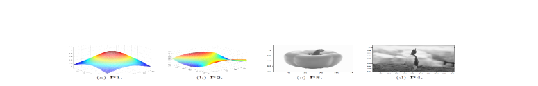
Figure 1: Test datasets.

Though our framework is readily applicable to image deblurring and image registration, here we only present denoising results.

7.1 Performance comparisons of boundary regularization

We first test the idea from §4. One the hand, the variational framework seeks the boundary conditions of a nonzero Dirichlet or a Neumann type on $\partial\Omega$ and also real images do have nonzero boundary conditions. On the other hand, fractional order derivatives require homogeneous boundary conditions (as used in works of many authors) due to end singularity. In order to aid accurate computation of the discretized fractional order derivative, in our work, a boundary processing technique §4 has been proposed to transform nonzero boundary conditions of observed data $z$ into zero boundary conditions; hence a consequent matrix approximation to the fractional derivative operator $D^{\alpha}_{[0,\;1]}$ can use a zero Dirichlet boundary condition.

Here we test the performance and effectiveness of our boundary regularization against no regularization. The experiment is carried out on P1 - Parabolic surfaces as shown in Fig. 2, i.e., a synthetic image of size $256\times 256$ and range [0, 1], in Fig. 2(a), which is added zero mean value Gaussian random noise with a mean variance $\delta=\frac{15}{256}$ to get the noisy image displayed in Fig. 2(d). For the boundary regularization case, the approximation $u|_{\partial\Omega}$ from the observed data $z|_{\partial\Omega}$ is from applying one dimensional fractional order variation model as described in §4. The treated case is named as ‘Treated’ whose results are depicted on Fig. 2(b) and Fig. 2(b)), where psnr$=47.53$ and snr=$35.43$. The solution obtained from assuming zero boundary conditions for $u$ is named as ‘Non-treated’ with its results depicted in Fig. 2(c) and Fig. 2(a), where $\emph{psnr}=23.69$ and $\emph{snr}=10.38$. Clearly our boundary regularization treatment is effective.

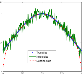
(a) Slice for non-treated - Bad.

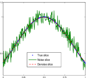
(b) Slice for treated - Good.

Figure 2: Test for P1—Comparisons between treated and Non-treated cases for non-zero boundary conditions ($\delta=\frac{15}{256}$) using PDE-SB. The treated case has psnr=$47.53$ and snr=$35.43$, while the non-treated case has psnr=$23.69$ and snr=$10.38$. Clearly our boundary regularization §4 is effective while direct application of a fractional model leads to incorrect boundary restoration. Here the error $r=\|u-u^{*}\|_{F}/\|u^{*}\|_{F}$.

7.2 Comparisons of Algorithms 1–4

In Table 1, we compare the restoration quality (via psnr and snr) of 4 Algorithms. There, all four test datasets are used. In the cases of synthetic images P1 and P2 with noise variation $\delta=\frac{10}{255}$, $\lambda$ is taken as $12000$ and $3800$ respectively and $\alpha=1.6$. In the cases of natural images P3 and P4 with noise variation $\delta=\frac{5}{255}$, $\lambda$ is taken as $18000$ and $20000$ respectively and $\alpha=1.4$. One can see that, from Table 1, Opti-Nesterov and PDE-SB perform similarly in terms of the best restoration quality (via psnr and snr). However in efficiency (computation times cpu(s)), Opti-FISTA and PDE-SB are the best while Opti-Nesterov takes more computational times than other three algorithms. Evidently, overall, PDE-SB (Algorithm 1) shows the most consistence in good performance in tested cases considered.

Table 1: Comparisons of optimizing Algorithms, where $\delta=\frac{10}{255}$ for saddle and parabolic surfaces, $\delta=\frac{5}{255}$ for pepper and penguin images.

Opti-FB Opti-Nesterov Opti-FISTA PDE-SB snr psnr cpu(s) snr psnr cpu(s) snr psnr cpu(s) snr psnr cpu(s) P1 36.78 50.09 16.83 36.91 50.22 27.23 36.94 50.24 16.71 36.96 50.27 14.53 P2 31.04 53.08 17.28 31.61 53.67 28.43 31.46 53.50 18.14 31.63 53.69 15.09 P3 29.21 43.29 15.96 29.40 43.49 16.09 29.40 43.49 9.75 29.48 43.56 8.16 P4 25.19 38.01 14.68 25.35 38.15 16.27 25.34 38.15 8.62 25.34 38.14 8.45

7.3 Sensitivity tests for $\alpha$ and $\lambda$

Since our model (16) contains two main parameters: $\alpha$ for the order of differentiation and $\lambda$ as the coupling parameter for a regularized inverse problem, it is of interest to test their sensitivity on the restoration quality. Here we shall test all Algorithms’s sensitivity using the image P2 - Saddle surface of size $256\times 256$, after adding zero mean value Gaussian random noise image of range [0, 1] and $\delta=\frac{10}{256}$.

Varying $\lambda$ in a large range from $400$ to $60000$, all four algorithms are tested on this synthetic image with the results shown in Figs. 3(a) and 3(c) for different stopping criterions (GSC: the general stopping criterions with the relative residual $10^{-4}$, relative error $10^{-8}$, inner iterations 10,SSC: the strong stopping criterions with the relative residual $10^{-7}$, relative error $10^{-10}$, inner iterations 25 ). Different from the TV denoising case where the regularization parameter $\lambda$ is crucial for restoration quality [82], however, Figs. 3(a) and 3(c) show that our total $\alpha$-order variation regularization model still obtains a satisfactory solution for a large range of $\lambda$; this is a pleasing observation. Of course there exists an issue of an optimal choice.

Next varying $\alpha\in(1,2)$ from $1.1$ to $1.9$, Figs. 3(b) and 3(d) show four algorithms’s restored results responding to two stopping conditions GSC and SSC. As represented, the smaller $\alpha$ leads to the blocky (staircase) effects in $u$ and the larger $\alpha$ will make solution $u$ too smooth along $x_{1}$- and $x_{2}$-directions respectively. For denoising, our test suggests that $\alpha=1.6$ is suitable for smooth problems because the diffusion coefficients are almost isotropic in all regions, leading to smooth deformation fields, and $\alpha=1.4$ is appropriate for nonsmooth problems because the diffusion coefficients are close to zero in regions representing large gradients of the fields, allowing discontinuities at those regions.

We should emphasize that the stopping criterions have impacted on the actual numerical implementation. In other words, if we drop the limit on the maximal number of inner iterations and relative residuals (and relative errors), some methods take too long but obtain the more satisfactory results.

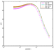
(a) GSC:psnr vs. $\lambda$

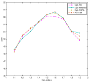
(b) GSC:psnr vs. $\alpha$

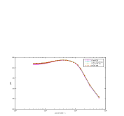
(c) SSC:psnr vs. $\lambda$

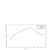
(d) SSC:psnr vs. $\alpha$

Figure 3: Sensitivity test of Algorithms 1-4 to parameters $\lambda$ (with the fixed $\alpha=1.6$) and $\alpha$ (with the fixed $\lambda=3800$) in the cases of the GSC and SSC stopping conditions.

7.4 Comparisons with other non-fractional variational models

In this test, we compare our total $\alpha$-variation model(PDE-SB) with three popular methods for variational image denoising. The first compared approach is naturally the TV model proposed by Rudin et al. [67] because the total $\alpha$-order variation model in this work is inspired by it. The second compared work is the mean curvature model [75] which also addresses the problem of restoring a good result for a smooth image; their approach is different from ours since it is focused on higher order regularization and a multigrid method. See also [53, 17, 84]. The third compared approach is the TGV model [15] involving a combination of first order and higher-order derivatives to reduce the staircasing effect of the bounded variation functional.

In Table 2, we first compare the restoration quality (via psnr, snr) and efficiency (computation times cpu(s)) of four approaches by testing the artificial images (P1 - Parabolic surface, P2 - saddle surface) and the natural images (P3 - Pepper, P4 - Penguin); in each approach relevant parameters are shown in Table 2. We see that, with the emperically optimal parameters $\lambda^{*}$, the differences of four models are very small, though our new and convex model is slightly better. In other tests where such optimal parameters are not used, our new model performs more robustly and better.

In order to present more visual differences, some stronger regularization parameters ($\lambda^{*}/2$) and higher noise variations (with the noise level $\delta=\frac{30}{255}$) are tested, the solution’s visual representations restoring the natural image P3 - Pepper in Fig. 4(b) are shown in Fig. 4. While ROF denoising leads to blocky results, the mean curvature model performs better in the smooth regions but exhibits more smooth near discontinuities, the total generalized variation model leads to further improvements over the aforementioned models. The total fractional-order variation model leads to significantly better results. The reason is that the new model tries to approximate the image based on affine functions or non-local high order smooth functions, which is clearly better in this case, in other words, our approach is more effective in eliminating the noise for smooth images and is competitive to high order methods; in efficiency the new approach (PDE-SB) is much faster than the TGV and the mean curvature. We also plot four error results between the restored and true images along a diagonal (magenta) line in Fig. 4(a) for comparison in Fig. 5; we see that PDE-SB produces the best restored surface, which show a major advantage (or better performance) of using our total $\alpha$-order variation model (16) when the test image is smooth, and even when the contrast between meaningful objects and the background is low.

Table 2: Comparisons of four models in restoration quality: the total $\alpha$ variation model (16), Mean Curvature [53, 17, 75], TV [67, 34, 23] and TGV [15] models for synthetic images (P1 and P2 in Fig. 1) and natural images (P3 in Fig. 4(a)) with different noise variances $\delta_{j}=\frac{\hat{\delta}_{j}}{255}$ (correspondingly we use $\lambda_{j}$). We first fix $\mu=1.1$, $\gamma=1$, $\alpha=1.6$ for P1-P2, $\alpha=1.15$ and $\alpha=1.1$ for P3-P4 respectively in the total $\alpha$-order variation model, and $\gamma=19$, $\beta=10^{-5}$ in the mean curvature model, and two weight parameters of the first and second order term in TGV model ($\nu_{0}=1$, $\nu_{1}=2$ for P1-P2, $\nu_{0}=1$, $\nu_{1}=0.5$ for P3-P4), other parameters are as shown on the “para” rows. $\lambda^{1D}$ from (19) is required by the new model only.

Mean curvature [75] TV [67] TGV [15] Total $\alpha$-order model (16) $\hat{\delta}$ snr psnr snr psnr snr psnr snr psnr $10$ 33.44 46.74 32.17 45.52 36.41 49.72 37.55 50.86 P1 $20$ 30.19 43.50 29.55 42.83 33.03 46.33 33.52 46.83 $\lambda_{1}=1/0.4\times 256^{2}$ $\lambda_{1}=1026$ $\lambda_{1}=1/1.2\times 256^{2}$ $\lambda^{1D}_{1}=0.1$, $\lambda_{1}=21900$ Para $\lambda_{2}=1/0.03\times 256^{2}$ $\lambda_{2}=535$ $\lambda_{2}=1/0.6\times 256^{2}$ $\lambda^{1D}_{2}=0.1$, $\lambda_{2}=14400$ $10$ 27.27 49.31 23.09 45.13 30.75 52.68 32.02 54.18 P2 $20$ 22.88 44.92 19.45 41.49 25.62 47.51 26.48 48.54 $\lambda_{1}=1/0.9\times 256^{2}$ $\lambda_{1}=883$ $\lambda_{1}=1/0.9\times 256^{2}$ $\lambda^{1D}_{1}=1$, $\lambda_{1}=1800$ Para $\lambda_{2}=1/0.01\times 256^{2}$ $\lambda_{2}=488$ $\lambda_{2}=1/0.5\times 256^{2}$ $\lambda^{1D}_{2}=0.2$, $\lambda_{2}=1800$ $10$ 20.43 38.80 20.08 38.35 20.40 38.78 20.48 38.86 $15$ 18.76 37.11 18.01 36.69 18.68 37.12 18.84 37.20 P3 $20$ 17.48 35.82 17.17 35.33 17.55 35.87 17.57 35.90 $\lambda_{1}=1/16\times 256^{2}$ $\lambda_{1}=2216$ $\lambda_{1}=1/55\times 256^{2}$ $\lambda^{1D}_{1}=1$, $\lambda_{1}=16500$ Para $\lambda_{2}=1/14\times 256^{2}$ $\lambda_{2}=1373$ $\lambda_{2}=1/26\times 256^{2}$ $\lambda^{1D}_{2}=0.1$, $\lambda_{2}=9300$ $\lambda_{3}=1/6\times 256^{2}$ $\lambda_{3}=893$ $\lambda_{3}=1/12\times 256^{2}$ $\lambda^{1D}_{3}=0.01$, $\lambda_{3}=6200$ $5$ 25.16 37.95 24.85 37.58 25.39 38.20 25.34 38.14 $10$ 21.72 34.60 21.33 34.07 21.82 34.71 21.75 34.62 P4 $15$ 19.26 32.05 18.66 31.29 19.44 32.21 19.42 32.20 $\lambda_{1}=1/9\times 256^{2}$ $\lambda_{1}=3341$ $\lambda_{1}=1/49\times 256^{2}$ $\lambda^{1D}_{1}=0.1$, $\lambda_{1}=24000$ Para $\lambda_{2}=1/5\times 256^{2}$ $\lambda_{2}=1856$ $\lambda_{2}=1/20\times 256^{2}$ $\lambda^{1D}_{2}=0.1$, $\lambda_{2}=8000$ $\lambda_{3}=1/6\times 256^{2}$ $\lambda_{3}=1095$ $\lambda_{3}=1/11\times 256^{2}$ $\lambda^{1D}_{3}=0.1$, $\lambda_{3}=18500$

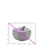
(a) True $z$.

(b) Noise $f$.

(c) TV.

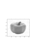
(d) Mean Curvature.

(e) TGV.

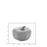
(f) Our Approach.

Figure 4: Comparison I —Comparisons of our PDE-SB with TV, mean curvature and TGV models.

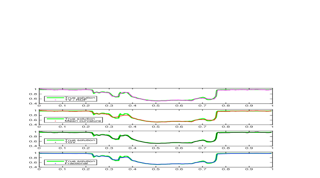
(a) $u$

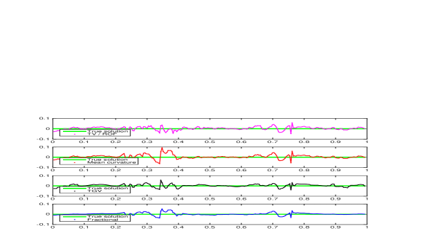
(b) error $u-u^{*}$

Figure 5: Comparison I — The slice presentations of four restorations along a diagonal line in Fig. 4(a).

8 Conclusions

The total $\alpha$-order variation regularization with fractional order derivative is potentially useful in modeling all imaging problems. In this paper we analyzed rigorously a simple variational model using total $\alpha$-order variation for image denoising. One Split-Bregman based algorithm and three optimization-based algorithms were developed to solve the resulting image inverse problem. Instead of using the usual fixed and zero boundary conditions, we proposed a boundary regularization method to treat the fractional order derivatives. Numerical results show that the PDE-based Split-Bregman algorithm (PDE-SB) performs similarly to (though more stably than) optimization-based approaches while our boundary regularization method is essential for getting good results for imaging denoising. Moreover, PDE-SB outperforms currently competitive variational models in terms of restoration quality. There are still outstanding issues with our proposed model and algorithms; among others optimal selection of $\lambda$ is to be addressed. Future work will also consider generalization of this work to other image inverse problems.

Appendix: Proof of Theorem 4

To shorten the proof, let $\omega$ be a function in $W_{1}^{\alpha}(\Omega)$ to be specified shortly. For $u\in W_{1}^{\alpha}(\Omega)\subset\text{BV}^{\alpha}(\Omega)$, we compute the first-order G-derivative (Gateaux) of the functional $J(u)$ in the direction $\omega$ by

$$\begin{split}J^{\prime}(u)\omega&=\lim\limits_{t\rightarrow 0}\frac{J(u+t\omega)-J(u)}{t}\ =\lim\limits_{t\rightarrow 0}\frac{Q(u+t\omega)-Q(u)}{t}+\frac{\lambda}{2}\frac{F(u+t\omega)-F(u)}{t}\end{split}$$ (32)

where $Q(u)=\frac{\mu}{2}\int_{\Omega}|\boldsymbol{d}-\nabla^{\alpha}u+\frac{\boldsymbol{p}}{\mu}|^{2}dx$ – see (22). Using the Taylor series w.r.t $t$ yields

$$J^{\prime}(u)\omega=\int_{\Omega}\boldsymbol{W}\cdot\nabla^{\alpha}\omega dx+\lambda\int_{\Omega}(u-z)\;\omega dx$$ (33)

with $\boldsymbol{W}=-\mu(\boldsymbol{d}-\nabla^{\alpha}u+\frac{\boldsymbol{p}}{\mu})$. Recall that

$$\begin{split}\int_{\Omega}\boldsymbol{W}\cdot\nabla^{\alpha}\omega dx=(-1)^{n}\int_{\Omega}\omega{}^{C}\text{div}^{\alpha}\boldsymbol{W}dx-&\sum_{j=0}^{n-1}(-1)^{j}\int_{0}^{1}D^{\alpha-n+j}_{[a,b]}W_{1}\frac{\partial^{n-j-1}\omega(x)}{\partial x_{1}^{n-j-1}}\Big{|}_{x_{1}=0}^{x_{1}=1}dx_{2}\\ -&\sum_{j=0}^{n-1}(-1)^{j}\int_{0}^{1}D^{\alpha-n+j}_{[c,d]}W_{2}\frac{\partial^{n-j-1}\omega(x)}{\partial x_{2}^{n-j-1}}\Big{|}_{x_{2}=0}^{x_{2}=1}dx_{1}.\end{split}$$ (34)

where we note $n=2$ for $1<\alpha<2$. Next consider 2 case studies.

i). Given $u(x)\big{|}_{\partial\Omega}=b_{1}(x),\ \text{and }\ \frac{\partial u(x)}{\partial n}\Big{|}_{\partial\Omega}=b_{2}(x)$, since $\big{(}u(x)+t\omega(x)\big{)}\big{|}_{\partial\Omega}=\big{(}u(x)\big{)}\big{|}_{\partial\Omega}=b_{1}(x)$ and $\frac{\partial\big{(}u(x)+t\omega(x)\big{)}}{\partial n}\Big{|}_{\partial\Omega}=\frac{\partial u(x)}{\partial n}\big{|}_{\partial\Omega}=b_{2}(x)$, it suffices to take $\omega\in\mathscr{C}_{0}^{1}(\Omega,\mathbb{R})$. Such a choice ensures $\frac{\partial^{i}\omega(x)}{\partial n^{i}}\Big{|}_{\partial\Omega}=0,i=0,1\ \ \Rightarrow\ \ \frac{\partial^{n-j-1}\omega(x)}{\partial x_{1}^{n-j-1}}\Big{|}_{x_{1}=0\ \mbox{or}\ 1}=\frac{\partial^{n-j-1}\omega(x)}{\partial x_{1}^{n-j-1}}\Big{|}_{x_{2}=0\ \mbox{or}\ 1}=0,\ n-j-1=0,1$. Hence equation (32) with (33) reduces to (23).

ii). Keep $\omega\in W_{1}^{\alpha}(\Omega)$. Since $\frac{\partial^{n-j-1}\omega(x)}{\partial x_{1}^{n-j-1}}\Big{|}_{x_{1}=0\ \mbox{or}\ 1}\not=0,\ \frac{\partial^{n-j-1}\omega(x)}{\partial x_{1}^{n-j-1}}\Big{|}_{x_{2}=0\ \mbox{or}\ 1}\not=0$, the boundary terms in equation (34) can only diminish if

$$D^{\alpha-n+j}_{[a,b]}W_{1}\Big{|}_{x_{1}=0\ \mbox{or}\ 1}=0\ \ \mbox{and}\ \ D^{\alpha-n+j}_{[c,d]}W_{2}\Big{|}_{x_{2}=0\ \mbox{or}\ 1}=0\ \ \Rightarrow\ \ D^{\alpha-n+j}\boldsymbol{W}\cdot n=0,j=0,1.$$

The proof is complete.

Remark 5

In imaging applications, the above first set i) of boundary conditions seems not reasonable, because one hardly knows a priori what $b_{1},b_{2}$ should be. The second set ii) of boundary conditions appears complicated which might be simplified as follows.

From [63, Section 2.3.6 pp.75], if $W_{1}(x)$ has a sufficient number of continuous derivatives, then
$D^{\alpha-n+j}_{[0,\;1]}W_{1}\Big{|}_{x_{1}=0\ \mbox{or}\ 1}=0$ for any $\alpha\in(1,2)$ is equivalent to $\frac{\partial^{j}W_{1}}{\partial x_{1}^{j}}\Big{|}_{x_{1}=0\ \mbox{or}\ 1}=0\;(j=0,1)$, i.e.,

$$W_{1}\Big{|}_{x_{1}=0\ \mbox{or}\ 1}=0\;\;\mbox{and}\;\;\frac{\partial W_{1}}{\partial x_{1}}\Big{|}_{x_{1}=0\ \mbox{or}\ 1}=0.$$

Indeed, if the $n$-th derivative of $u(x)$ is integrable in $[0,1]$, then $W_{1}\Big{|}_{x_{1}=0\ \mbox{or}\ 1}=0$ is equivalent to

$$u(x)\Big{|}_{x_{1}=0\ \mbox{or}\ 1}=0\;\;\mbox{and}\;\;\frac{\partial u(x)}{\partial x_{1}}\Big{|}_{x_{1}=0\ \mbox{or}\ 1}=0;$$

on the other hand, $\frac{\partial^{k}u(x)}{\partial x_{1}^{k}}\Big{|}_{x_{1}=0\ \mbox{or}\ 1}=0$ (for all $k=0,1,2$) are equivalent to $\frac{\partial^{\alpha}u(x)}{\partial x_{1}^{\alpha}}\Big{|}_{x_{1}=0\ \mbox{or}\ 1}=0$ and $\frac{\partial^{1+\alpha}u(x)}{\partial x_{1}^{1+\alpha}}\Big{|}_{x_{1}=0\ \mbox{or}\ 1}=0$, hence one has $\frac{\partial W_{1}}{\partial x_{1}}\Big{|}_{x_{1}=0\ \mbox{or}\ 1}=0$. The derivations of $W_{2}$ are similar to those of $W_{1}$.

For related papers or Matlab codes, see Authors’ page:   http:\\www.liv.ac.uk/~cmchenke

References

- [1] R. Acar and C. R. Vogel, Analysis of bounded variation penalty methods for ill-posed problems, Inverse Problems, 10 (1994), pp. 1217–1229.
- [2] V. Agarwal, A. V. Gribok, and M. A. Abidi, Image restoration using l-1 norm penalty function, Inverse Problems in Science and Engineering, 15 (2007), pp. 785–809.
- [3] O. P. Agrawal, Formulation of Euler-Lagrange equations for fractional variational problems, J. Math. Anal. Appl., 272 (2002), pp. 368 – 379.
- [4] , Fractional variational calculus in terms of Riesz fractional derivatives, Journal of Physics A: Mathematical and Theoretical, 40 (2007), pp. 62–87.
- [5] R. Almeida and D. F. M. Torres, Calculus of variations with fractional derivatives and fractional integrals, Applied Mathematics Letters, 22 (2009), pp. 1816–1820.
- [6] , Necessary and sufficient conditions for the fractional calculus of variations with caputo derivatives, Communications in Nonlinear Science and Numerical Simulation, 16 (2011), pp. 1490–1500.
- [7] L. Ambrosio and S. Masnou, A direct variational approach to a problem arising in image reconstruction, Interfaces and Free Boundaries, 5 (2003), pp. 63–82.
- [8] A. Atangana and A. Secer, A note on fractional order derivatives and table of fractional derivatives of some special functions, Abstract and Applied Analysis, 2013 (2013).
- [9] G. Aubert and P. Kornprobst, Mathematical Problems in Image Processing: Partial Differential Equations and the Calculus of Variations, vol. 147, Springer-Verlag, 2006.
- [10] J. F. Aujol, Some first-order algorithms for total variation based image restoration, Journal of Mathematical Imaging and Vision, 34 (2009), pp. 307–327.
- [11] J. Bai and X.-C. Feng, Fractional-order anisotropic diffusion for image denoising, IEEE Transactions on Image Processing, 16 (2007), pp. 2492–2502.
- [12] H. H. Bauschke, R. S. Burachik, P. L. Combettes, V. Elser, D. R. Luke, and H. Wolkowicz, Fixed-point algorithms for inverse problems in science and engineering, vol. 49, Springer Science & Business Media, 2011.
- [13] A. Beck and M. Teboulle, Fast gradient-based algorithms for constrained total variation image denoising and deblurring problems, Image Processing, IEEE Transactions on, 18 (2009), pp. 2419–2434.
- [14] , A fast iterative shrinkage-thresholding algorithm for linear inverse problems, SIAM Journal on Imaging Sciences, 2 (2009), pp. 183–202.
- [15] K. Bredies, K. Kunisch, and T. Pock, Total generalized variation, SIAM Journal on Imaging Sciences, 3 (2010), pp. 492–526.
- [16] X. Bresson, S. Esedoglu, P. Vandergheynst, J.-P. Thiran, and S. Osher, Fast global minimization of the active contour/snake model, Journal of Mathematical Imaging and Vision, 28 (2007), pp. 151–167.
- [17] C. Brito-Loeza and K. Chen, Multigrid algorithm for high order denoising, SIAM J. Imaging Sci., 3 (2010), pp. 363–389.
- [18] A. Chambolle, An algorithm for total variation minimization and applications, Journal of Mathematical Imaging and Vision, 20 (2004), pp. 89–97.
- [19] A. Chambolle and P. L. Lions, Image recovery via total variation minimization and related problems, Numerische Mathematik, 76 (1997), pp. 167–188.
- [20] A. Chambolle and T. Pock, A first-order primal-dual algorithm for convex problems with applications to imaging, Journal of Mathematical Imaging and Vision, 40 (2011), pp. 120–145.
- [21] R. H. Chan, A. Lanza, S. Morigi, and F. Sgallari, An adaptive strategy for the restoration of textured images using fractional order regularization, Numer. Math. Theor. Meth. Appl., 6 (2013), pp. 276–296.
- [22] T. Chan, A. Marquina, and P. Mulet, High-order total variation-based image restoration, SIAM Journal on Scientific Computing, 22 (2000), pp. 503–516.
- [23] T. Chan and J. Shen, Image Processing And Analysis: Variational, PDE, Wavelet, and Stochastic Methods, SIAM, 2005.
- [24] T. Chan, A. M. Yip, and F. E. Park, Simultaneous total variation image inpainting and blind deconvolution, International Journal of Imaging Systems and Technology, 15 (2005), pp. 92–102.
- [25] Q. S. Chang, X. C. Tai, and L. Xing, A compound algorithm of denoising using second-order and fourth-order partial differential equations, Numerical Mathematics: Theory, Methods and Applications, 2 (2009), pp. 353–376.
- [26] D. Chen, Y. Chen, and D. Xue, Fractional-order total variation image restoration based on primal-dual algorithm, Abstract and Applied Analysis, 2013 (2013), p. 585310.
- [27] , Three fractional-order TV- models for image denoising, Journal of Computational Information Systems, 9 (2013), pp. 4773– 4780.
- [28] D. Chen, S. S. Sun, C. R. Zhang, Y. Q. Chen, and D. Y. Xue, Fractional-order TV-L2 model for image denoising, Central European Journal of Physics, 11 (2013), pp. 1414–1422.
- [29] N. Chumchob, K. Chen, and C. Brito-Loeza, Fourth order variational image registration on model and its fast multigrid algorithm, SIAM Multiscale Model. Simul., 9 (2011), pp. 89–128.
- [30] P. L. Combettes and V. R. Wajs, Signal recovery by proximal forward-backward splitting, Multiscale Modeling & Simulation, 4 (2005), pp. 1168–1200.
- [31] G. Dal-Maso, I. Fonseca, G. Leoni, and M. Morini, A higher order model for image restoration: The one-dimensional case, SIAM Journal on Mathematical Analysis, 40 (2009), pp. 2351–2391.
- [32] V. Duval, J. F. Aujol, and L. Vese, Projected Gradient Based Color Image Decomposition, vol. 5567 of Lecture Notes in Computer Science, 2009, pp. 295–306.
- [33] L. C. Evans and R. F. Gariepy, Measure theory and fine properties of functions, vol. 5, CRC press, 1991.
- [34] R. P. Fedkiw, G. Sapiro, and C. W. Shu, Shock capturing, level sets, and pde based methods in computer vision and image processing: a review of osher’s contributions, Journal of Computational Physics, 185 (2003), pp. 309–341.
- [35] B. Fischer and J. Modersitzki, Fast diffusion registration, Contemporary Mathematics, 313 (2002), pp. 117–128.
- [36] , Curvature based image registration, Journal of Mathematical Imaging and Vision, 18 (2003), pp. 81–85.
- [37] C. Frohn-Schauf, S. Henn, and K. Witsch, Multigrid based total variation image registration, Computing and Visualization in Science, 11 (2008), pp. 101–113.
- [38] J. B. Garnett, T. M. Le, Y. Meyer, and L. A. Vese, Image decompositions using bounded variation and generalized homogeneous besov spaces, Applied and Computational Harmonic Analysis, 23 (2007), pp. 25–56.
- [39] S. Geman and D. Geman, Stochastic relaxation, gibbs distributions, and the bayesian restoration of images, IEEE Trans. Pattern Analysis and Machine Intelligence, 6 (1984), pp. 721–741.
- [40] P. Getreuer, Total variation inpainting using split Bregman, Image Processing On Line, 2 (2012), p. 147–157.
- [41] S. N. Ghate, S. Achaliya, and S. Raveendran, An algorithm of total variation for image inpainting, International Journal of Computer & Electronics Research, 1 (2012), pp. 124–130.
- [42] E. Giusti, Minimal Surfaces and Functions of Bounded Variation, Springer, 1984.
- [43] T. Goldstein and S. Osher, The split Bregman method for L1-regularized problems, SIAM Journal on Imaging Sciences, 2 (2009), pp. 323–343.
- [44] P. Guidotti, A new nonlocal nonlinear diffusion of image processing, Journal of Differential Equations, 246 (2009), pp. 4731–4742.
- [45] P. Guidotti and J. V. Lambers, Two new nonlinear nonlocal diffusions for noise reduction, Journal of Mathematical Imaging and Vision, 33 (2009), pp. 25–37.
- [46] W. Guo and L. H. Qiao, Inpainting based on total variation, in International Conference on Wavelet Analysis and Pattern Recognition, vol. 2, 2007, pp. 939–943.
- [47] R. Hilfer, Applications of Fractional Calculus in Physics, World Scientific, 2000.
- [48] L. Hömke, C. Frohn-Schauf, S. Henn, and K. Witsch, Total variation based image registration, in Image Processing Based on Partial Differential Equations, Springer, 2007, pp. 343–361.
- [49] M. Janev, S. Pilipović, T. Atanacković, R. Obradović, and N. Ralević, Fully fractional anisotropic diffusion for image denoising, Mathematical and Computer Modelling, 54 (2011), pp. 729–741.
- [50] G. Jumarie, Modified riemann-liouville derivative and fractional taylor series of nondifferentiable functions further results, Computers & Mathematics with Applications, 51 (2006), pp. 1367–1376.
- [51] H. Köstler, K. Ruhnau, and R. Wienands, Multigrid solution of the optical flow system using a combined diffusion-and curvature-based regularizer, Numerical Linear Algebra with Applications, 15 (2008), pp. 201–218.
- [52] M. Lysaker, A. Lundervold, and X. C. Tai, Noise removal using fourth-order partial differential equation with application to medical magnetic resonance images in space and time, IEEE Transactions on Image Processing, 12 (2003), pp. 1579–1590.
- [53] M. Lysaker, S. Osher, and X. C. Tai, Noise removal using smoothed normals and surface fitting, IEEE Transactions on Image Processing, 13 (2004), pp. 1345–1357.
- [54] A. Melbourne, N. Cahill, C. Tanner, M. Modat, D. J. Hawkes, and S. Ourselin, Using fractional gradient information in non-rigid image registration: application to breast MRI, Proc. SPIE, 2012.
- [55] K. S. Miller and B. Ross, An Introduction to the Fractional Calculus and Fractional Differential Equations, Wiley Interscience Publication, Wiley, 1993.
- [56] J. Modersitzki, Numerical Methods for Image Registration, Oxford University Press, 2004.
- [57] Y. Nesterov, A method for unconstrained convex minimization problem with the rate of convergence , in Soviet Mathematics Doklady, vol. 269, 1983, pp. 543–547.
- [58] , Gradient methods for minimizing composite functions, Mathematical Programming, 140 (2013), pp. 125–161.
- [59] K. B. A. Oldham and J. A. Spanier, The Fractional Calculus: Theory And Applications of Differentiation And Integration to Arbitrary Order, Dover Publications, 2006.
- [60] S. Osher, M. Burger, D. Goldfarb, J. J. Xu, and W. T. Yin, An iterative regularization method for total variation-based image restoration, Multiscale Modeling & Simulation, 4 (2005), pp. 460–489.
- [61] S. Osher, A. Sole, and L. Vese, Image decomposition and restoration using total variation minimization and the H-1 norm, Multiscale Modeling & Simulation, 1 (2003), pp. 349–370.
- [62] T. Pock, M. Urschler, C. Zach, R. Beichel, and H. Bischof, A duality based algorithm for TV-L1-optical-flow image registration, in Medical Image Computing and Computer-Assisted Intervention, Springer, 2007, pp. 511–518.
- [63] I. Podlubny, Fractional Differential Equations: An Introduction to Fractional Derivatives, Fractional Differential Equations, to Methods of Their Solution and Some of Their Applications, Mathematics in Science and Engineering, Elsevier Science, 1999.
- [64] , Matrix approach to discrete fractional calculus, Fractional Calculus and Applied Analysis, 3 (2000), pp. 359–386.
- [65] I. Podlubny, A. Chechkin, T. Skovranek, Y. Chen, and B. M. Vinagre-Jara, Matrix approach to discrete fractional calculus ii: Partial fractional differential equations, Journal of Computational Physics, 228 (2009), pp. 3137–3153.
- [66] P. D. Romero and V. F. Candela, Blind deconvolution models regularized by fractional powers of the laplacian, Journal of Mathematical Imaging and Vision, 32 (2008), pp. 181–191.
- [67] L. Rudin, S. Osher, and E. Fatemi, Nonlinear total variation based noise removal algorithms, Physica D: Nonlinear Phenomena, 60 (1992), pp. 259–268.
- [68] S. G. Samko, A. A. Kilbas, and O. I. Marichev, Fractional integrals and derivatives: Theory and Applications, CRC Press, 1993.
- [69] O. Scherzer, M. Grasmair, H. Grossauer, M. Haltmeier, and F. Lenzen, Variational Methods in Imaging, Applied Mathematical Sciences, Springer, 2009.
- [70] S. Setzer, Split Bregman Algorithm, Douglas-Rachford Splitting and Frame Shrinkage, vol. 5567 of Lecture Notes in Computer Science, 2009, pp. 464–476.
- [71] , Operator splittings, Bregman methods and frame shrinkage in image processing, International Journal of Computer Vision, 92 (2011), pp. 265–280.
- [72] J. Shen, S. H. Kang, and T. Chan, Euler’s elastica and curvature-based inpainting, SIAM Journal on Applied Mathematics, 63 (2003), pp. 564–592.
- [73] Z. W. S. Shen, K. C. Toh, and S. Yun, An accelerated proximal gradient algorithm for frame-based image restoration via the balanced approach, SIAM Journal on Imaging Sciences, 4 (2011), pp. 573–596.
- [74] G. Steidl, S. Didas, and J. Neumann, Relations between higher order TV regularization and support vector regression, vol. 3459 of Lecture Notes in Computer Science, 2005, pp. 515–527.
- [75] L. Sun and K. Chen, A new iterative algorithm for mean curvature-based variational image denoising, BIT Numerical Mathematics, 54 (2014), pp. 523–553.
- [76] A. N. Tikhonov and V. Y. Arsenin, Solutions of ill-posed problems, John Wiley & Sons, 1977.
- [77] M. Unger, T. Pock, W. Trobin, D. Cremers, and H. Bischof, TVSeg-interactive total variation based image segmentation, in BMVC, 2008 British Machine Vision Conference (Leeds), 2008, pp. 1–10.
- [78] R. Verdú-Monedero, J. Larrey-Ruiz, J. Morales-Sánchez, and J. L. Sancho-Gómez, Fractional regularization term for variational image registration, Mathematical Problems in Engineering, 2009 (2009), p. 707026.
- [79] H. Wang and N. Du, Fast solution methods for space-fractional diffusion equations, Journal of Computational and Applied Mathematics, 255 (2014), pp. 376–383.
- [80] E. Zeidler, Nonlinear functional analysis and its applications III: Variational methods and optimization, Springer-Verlag, New York, 1985.
- [81] J. Zhang, Z. Wei, and L. Xiao, Adaptive fractional-order multi-scale method for image denoising, Journal of Mathematical Imaging and Vision, 43 (2012), pp. 39–49.
- [82] J. P. Zhang, K. Chen, and B. Yu, An iterative Lagrange multiplier method for constrained total-variation-based image denoising, SIAM Journal on Numerical Analysis, 50 (2012), pp. 983–1003.
- [83] Y. Zhang, Y. F. Pu, J. R. Hu, and J. L. Zhou, A class of fractional-order variational image inpainting models, Appl. Math. Inf. Sci, 6 (2012), pp. 299–306.
- [84] W. Zhu and T. F. Chan, Image denoising using mean curvature of image surface, SIAM Journal on Imaging Sciences, 5 (2012), pp. 1–32.
- [85] Z. Y. Zhu, G. G. Li, and C. J. Cheng, A numerical method for fractional integral with applications, Applied Mathematics and Mechanics, 24 (2003), pp. 373–384.