Discrete dynamics and non-Markovianity

Abstract

We study discrete quantum dynamics where single evolution step consists of unitary system transformation followed by decoherence via coupling to an environment. Often non-Markovian memory effects are attributed to structured environments whereas here we take a more general approach within discrete setting. In addition of controlling the structure of the environment, we are interested in how local unitaries on the open system allow the appearance and control of memory effects. Our first simple qubit model, where local unitary is followed by dephasing, illustrates how memory effects arise despite of having no-structure in the environment the system is coupled with. We then elaborate this observation by constructing a model for open quantum walk where the unitary coin and transfer operation is augmented with dephasing of the coin. The results demonstrate that in the limit of strong dephasing within each evolution step, the combined coin-position open system always displays memory effects and their quantity is independent of the structure of the environment. Our construction makes possible an experimentally realizable open quantum walk with photons exhibiting non-Markovian features.

I Introduction

In recent years, there has been a growing interest on defining and quantifying quantum memory effects in open system dynamics Wolf et al. (2008); Breuer et al. (2009); Rivas et al. (2010); Lu et al. (2010); Luo et al. (2012); Lorenzo et al. (2013); Bylicka et al. (2014); Chruściński and Maniscalco (2014); Buscemi and Datta (2014); Breuer et al. (2015). These are based on a number of different approaches, ranging, e.g., from the concepts of information flow Breuer et al. (2009), to non-divisibility Rivas et al. (2010); Chruściński and Maniscalco (2014) and mutual information Luo et al. (2012). Based on these theoretical developments, experimental realizations for detecting and controlling of non-Markovianity has become feasible Liu et al. (2014, 2011) and also a number of proposals to exploit memory effects, e.g., to quantum information tasks has been recently proposed Vasile et al. (2011); Bylicka et al. (2014, 2015). The previous studies on non-Markovian quantum dynamics mostly focus on continuous coupling between the open system and its environment. However, there also exists other possibilities to study memory effects, for example discrete dynamics which we consider here. In this case, the open system couples in stepwise manner in time to its environment. One can also envisage a possibility of having unitary transformations changing the state of the open systems between non-unitary evolution steps caused by the environment. We are interested in what is the state of the open system after each step which consists consecutive unitary and non-unitary parts. Thereby, the theoretical challenge is to construct a discrete dynamical map for the stepwise evolution of the system of interest and this map should contain information about the local unitary within the system of interest and the properties of the environment it is interacting with.

Quantum walks provide a promising base to combine the study of discrete dynamics and memory effects. Generally, in quantum walks the system can evolve discretely or continuously Venegas-Andraca (2012); Aharonov et al. (2000); Kempe (2003) and a study on the relation between the two cases can be found in Strauch (2006). Quantum walks have proven to be important in such diverse fields as quantum information processing Lovett et al. (2010), complex networks Caruso (2014); Faccin et al. (2013) and the physics of topological phases Kitagawa (2012); Puentes et al. (2014). Moreover, the dynamics of quantum walks show a very broad range of different dynamical behavior from ballistic spreading to localization Ghosh (2014); Crespi et al. (2013); Chandrashekar (2012); Jackson et al. (2012); Schreiber et al. (2011); Ahlbrecht et al. (2011a, b); Kendon (2006); Tregenna et al. (2003). Introducing noise to the quantum walk, the effects of the transition from unitary to non-unitary dynamics and the classical limit can be studied Venegas-Andraca (2012); Attal et al. (2012a, b); Schreiber et al. (2011); Ahlbrecht et al. (2011b); Lavička et al. (2011); Fan et al. (2011); Broome et al. (2010); Maloyer and Kendon (2007); Kendon (2007); Košík et al. (2006); Ermann et al. (2006); Brun et al. (2003a, b, c); Kendon and Tregenna (2003, 2002). Recently, quantum walks have been implemented experimentally for example using trapped ions Zähringer et al. (2010); Karski et al. (2009), atoms in optical lattices Robens et al. (2015), linear optics Puentes et al. (2014); Broome et al. (2010), optical fibers Schreiber et al. (2011, 2010) and waveguides Crespi et al. (2013); Sansoni et al. (2012); Perets et al. (2008).

In this article we study non-Markovian discrete dynamics of discrete quantum walk in a line. For this purpose, we introduce a new type open quantum walk where the dynamics is characterized by a non-divisible discrete dynamical map. It is worth pointing out that, to the best of our knowledge, all previous approaches to decoherent quantum walks can be characterized by using discrete quantum dynamical semigroup. We go beyond dynamics which is describable by semigroup and are interested in how to induce and control memory effects for quantum walks. The article is structured in the following way. We first introduce the concept of discrete dynamical map and also formulate the suitable quantifier for memory effects. To understand better the origin of memory effects in the considered models, we then review the standard dephasing model for a qubit with non-Markovian dynamics. We then study discrete open qubit dynamics with unitary control operation and show how the addition of the control transforms the dynamics of the open system inherently non-Markovian. The elaborate on the insights obtained from the simple qubit model, we construct a discrete quantum walk where we identify the coin operator as the local control operation and proceed with memory effects in 1-d discrete open quantum walk. Throughout this paper the interaction between the open system and its environment is of pure dephasing type and in the quantum walk model the coin is coupled to an environment. The formulation follows the path and emphasis the experimental realization of the models with photons.

II Discrete dynamical map

Quantum dynamics is generated by quantum dynamical maps, a family of completely positive and trace preserving (CPT) maps $\Phi_{n}$ , $n\geq 0$, such that $\Phi_{0}=\mathbb{I}$ . If the state of the quantum system, described by a density operator or matrix, is initially $\rho_{0}$ then $\rho_{n}=\Phi_{n}(\rho_{0})$ defines the evolution of the state. Discrete dynamics for a quantum system emerge if the parameter $n$ indexing the family of CPT maps $\Phi_{n}$ takes discrete values only, eg. $n\in\mathbb{N}$. We assume that $0\in\mathbb{N}$.

CPT maps suitable for studying discrete dynamics can be constructed by using the Stinespring’s dilation theorem Heinosaari and Ziman (2011). It states that for every CPT map it is possible to assign an unitary evolution in enlarged Hilbert space. Total Hilbert space is thus $\mathcal{H}=\mathcal{H}_{\mathcal{S}}\otimes\mathcal{H}_{\mathcal{E}}$ and the map is generated as $\rho_{n}={\rm tr}_{\mathcal{E}}\{U^{n}\rho_{0}\otimes\chi(U^{\dagger})^{n}\}$. Here $U$ is unitary operator acting on total Hilbert space and $\chi$ is fixed initial state on the auxiliary Hilbert space. This construction guarantees that $\Phi_{n}$ is CPT for each $n$. Physical interpretation for this construction in the context of open quantum systems is that $\mathcal{H}_{\mathcal{E}}$ is a Hilbert space for external environment to which the system is coupled unitarily.

Quantum dynamical maps can be classified in the following way by their divisibility properties. If the dynamical map $\Phi_{n}$ satisfies the following decomposition law

$$\Phi_{n+m}(t)= \Phi_{n}\circ\Phi_{m},$$ (1)

for all $n\in\mathbb{N}$, then the dynamical map is Markovian and forms a discrete dynamical semigroup. The dynamical map is called CP-divisible if

$$\Phi_{n+m}=W_{n+m,m}\circ\Phi_{m},$$ (2)

for $n,m\in\mathbb{N}$ and where $W_{n+m,m}$ is completely positive and trace preserving. If the dynamical map can be composed as

$$\Phi_{n+m}= V_{n,m}\circ\Phi_{m},$$ (3)

where $V_{n,m}$ is positive and trace preserving then the dynamical map is called P-divisible Vacchini et al. (2011).

It is clear that the divisibility property of the dynamical map goes beyond the concept of semigroup. However, the various definitions of quantum non-Markovianity are still under active discussion Breuer et al. (2015). In the next section we will introduce the measure used in this work to quantify non-Markovianity of the discrete dynamical map.

III Measure for non-Markovianity

Following Breuer et al. (2009), we use a measure based on distinguishability of quantum states, quantified by the trace distance $d(\rho_{1},\rho_{2})=\frac{1}{2}{\rm tr}|\rho_{1}-\rho_{2}|$. Trace distance is contractive under positive and trace preserving maps Pérez-García et al. (2006), hence also under completely positive and trace preserving maps. Thus, the evolution of trace distance for fixed initial pair under P-divisible map is contractive, which means that $D_{\rho_{1},\rho_{2}}(m)\geq D_{\rho_{1},\rho_{2}}(n)$ for all $m<n$ where $D_{\rho_{1},\rho_{2}}(n)=d(\Phi_{n}\rho_{1},\Phi_{n}\rho_{2})$. If we find that the trace distance increases, $D_{\rho_{1},\rho_{2}}(n)>D_{\rho_{1},\rho_{2}}(m)$ for some $n>m$, then we know that the dynamical map is not P-divisible and we say that the dynamics is non-Markovian.

To construct a measure for discrete dynamics, we define the increment of the trace distance evolution

$$\Delta_{1,2}(n)= D_{\rho_{1},\rho_{2}}(n)-D_{\rho_{1},\rho_{2}}(n-1),\,n\geq 1,$$

$$\Delta_{1,2}(0)= 0,$$

and the measure for non-Markovianity is defined in terms of the increment as

$$\mathcal{N}(\Phi)(n)= \max_{\rho_{1},\rho_{2}}\sum_{n\in S=\{n\in\mathbb{N}|\Delta_{1,2}(n)>0\}}\Delta_{1,2}(n)$$ (4)

It can be shown that it is sufficient to make the maximization over orthogonal pairs of states  Wißmann et al. (2012) and it also has a local representation Liu et al. (2014). The measure has physical interpretation in terms of information flow between the system and the environment. When $\Delta_{1,2}(n)<0$ information flows away from the system to the environment and the ability to distinguish the two states decreases. When $\Delta_{1,2}(n)>0$ there is a backflow of information from the environment to the system which improves the distinguishability. In general, a lower bound for non-Markovianity is quite straightforward to obtain using only a small number of initial states. It is also worth noting that there exists evolutions which are not P-divisible but the trace distance between evolving states might still decrease at all points of time. In this work we do not present the results for full optimization over all the initial states but instead focus on specific pairs of initial states which allow to witness the non-Markovianity of the dynamics.

IV Discrete qubit dynamics

IV.1 Dephasing

Genuine quantum effect on open quantum system dynamics is the loss of quantum coherences without energy exchange between the system and the environment. This effect is called pure dephasing. Our motivation to study this effect on qubit dynamics is due to possibility of experimental implementation using optical elements Liu et al. (2011). Coupling between the system and the environment is given by

$$U_{\delta t}= \int{\rm d}\omega\sum_{\nu=L,R}e^{in_{\nu}\omega\delta t}|\nu\rangle\langle\nu|\otimes|\omega\rangle\langle\omega|,$$ (5)

where $|\nu\rangle$ labels the qubit degree of freedom and $|\omega\rangle$ corresponds to the environmental degree of freedom. With an optical implementation in mind, this type of unitary dynamics describes the interaction of a photon with a birefringent medium, eg. quartz Liu et al. (2011). Different basis states $|\nu\rangle$ correspond to the different polarization states, $n_{\nu}$ is the polarization dependent index of refraction, $\omega$ is the frequency of the photon and $\delta t$ corresponds to the thickness of the quartz plate.

For a fixed product initial state $\varrho=\rho(0)\otimes\chi$ this coupling generates pure dephasing dynamics, given by a dynamical map $\Phi_{\delta t}^{\rm PD}\rho(0)=\text{tr}_{\mathcal{E}}\left\{U_{\delta t}\varrho U_{\delta t}^{\dagger}\right\}$, expressed in $|\nu\rangle$ basis as

$$\Phi_{\delta t}^{\rm PD}: \left\{\begin{array}[]{ll}|\nu\rangle\langle\nu|&\mapsto|\nu\rangle\langle\nu|,\,\forall\nu,\\ |L\rangle\langle R|&\mapsto\kappa(\delta t)|L\rangle\langle R|,\\ |R\rangle\langle L|&\mapsto\kappa^{*}(\delta t)|R\rangle\langle L|\end{array}\right.$$ (9)

The map is determined by the the function $\kappa:\mathbb{R}_{+}\mapsto\mathbb{C}$, $\kappa(\delta t)=\int{\rm d}\omega e^{i\Delta n\omega\delta t}|\chi(\omega)|^{2}$, where $\Delta n=n_{L}-n_{R}$. Throughout this work we take the environment initial population distribution $|\chi(\omega)|^{2}$ (spectrum) to be constructed of two Gaussians with widths $\sigma$, amplitudes $\frac{A}{1+A}$ and $\frac{1}{1+A}$, where $A\in[0,1]$, central frequencies of the peaks $\mu_{1},\mu_{2}$ and peak separation $\delta\omega=\mu_{2}-\mu_{1}$, so that

$$|\chi(\omega)|^{2}= \frac{1}{1+A}\left(\frac{1}{\sqrt{2\pi\sigma^{2}}}\right)\left(e^{(\omega-\mu_{1})^{2}/(2\sigma^{2})}+Ae^{(\omega-\mu_{2})^{2}/(2\sigma^{2})}\right).$$ (10)

This choice is experimentally motivated Liu et al. (2011) and with parameters $A$ and $\sigma$ it is possible to control the structure of the environment.

It can be shown that the dynamics over a period $\delta t$ can be Markovian or non-Markovian depending on the properties of the population distribution $|\chi(\omega)|^{2}$ of the initial state of the environment. Dynamics as a function of $\delta t\equiv t$ is plotted in Fig. 1. Trace distance dynamics for the optimal pair of initial states is given by $D_{\rho_{1},\rho_{2}}(\delta t)=|\kappa(\delta t)|$. This type of dynamics is analyzed in Liu et al. (2011).

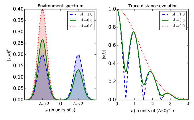
Figure 1: Standard dephasing model for a qubit. On the left is plotted the spectrum of the environment, it consists of Gaussian peaks. On the right is plotted the trace distance dynamics for maximizing initial state pair. As one can see, the single Gaussian peak gives Markovian dynamics and more structured environment gives rise to quantum memory effects. Here $\Omega=\delta\omega/(2\pi)$.

IV.2 Dephasing with local control

We consider now discrete dynamics where at each step in the dilatation space we have an action of a local control unitary operation Berglund (2000) followed by dephasing. The single step unitary in the total space is then

$$V=U_{\delta t}\cdot(C_{\eta}\otimes I_{\mathcal{E}}).$$ (11)

In this work we consider only the following local control unitaries $C_{\eta}$

$$C_{\eta}= \sqrt{\eta}(|L\rangle\langle L|-|R\rangle\langle R|)+\sqrt{1-\eta}(|L\rangle\langle R|+|R\rangle\langle L|).$$ (12)

These correspond to biased beam splitter transformations and $\eta=\frac{1}{2}$ being the Hadamard transformation also known as the balanced beam splitter transformation. The local unitary operator transforms the polarization basis into a new basis which is not generally simultaneously diagonalizable with the decoherence basis. This proves to be crucial for the non-Markovianity of the quantum dynamics as we will show. The reduced dynamics generated by $V^{n}$ is given by $\Phi_{n}^{\rm Q}$ which is defined as

$$\rho(n)=\Phi_{n}^{\rm Q}\rho= \text{tr}_{\mathcal{E}}\left\{V^{n}(\rho\otimes\chi)(V^{\dagger})^{n}\right\}.$$ (13)

The state of the qubit can be expressed as $\rho=\frac{1}{2}(\mathbb{I}_{2}+\vec{r}\cdot\vec{\sigma})$, where $\vec{r}=(r_{1},r_{2},r_{3})^{T}$ is the Bloch vector and $\vec{\sigma}=(\sigma_{1},\sigma_{2},\sigma_{3})^{T}$ where $\sigma_{i}$ are the usual Pauli matrices. For arbitrary values of $\eta$ the dynamics is most conveniently given in terms of the Bloch vector. The dynamical map can be written as

$$\vec{r}(m)= \int d\omega|\chi(\omega)|^{2}M(\omega)^{m}\vec{r}.$$ (14)

The matrix $M(\omega)$ is given by

$$M(\omega)= \begin{pmatrix}-\beta\cos{\Delta n\delta t\omega}&-\sin(\Delta n\delta t\omega)&\alpha\cos{\Delta n\delta t\omega}\\ \beta\sin{\Delta n\delta t\omega}&-\cos{\Delta n\delta t\omega}&-\alpha\sin{\Delta n\delta t\omega}\\ \alpha&0&\beta\end{pmatrix},$$ (16)

where $\alpha=2\sqrt{(1-\eta)\eta}$, $\beta=2\eta-1$ and $\Delta n=n_{L}-n_{R}$. Matrix $M(\omega)$ is periodic, eg. $M(\omega+\tilde{\Omega})=M(\omega)$, where $\tilde{\Omega}=\frac{2\pi}{\delta t\Delta n}$. Numerical integration of $M(\omega)^{m}$ must be done carefully since integrands are highly oscillatory. However, reliable numerical results can be obtained. In the strong dephasing limit, $\tilde{\Omega}\ll\sigma$ and for some particular values of $\eta$ it is possible to obtain analytical results.

Figures  2 and 3 present the results for the values $\eta=0,0.5,1.0$ in the case of weak and intermediate dephasing strength. It is worth noting that for all of the cases we have $A=0$, i.e., the environmental spectrum is flat corresponding to Markovian dynamics without local control.

For $\eta=1$, the local control is $C_{1}=\sigma_{z}$ and we have

$$\langle\nu,\omega|(U_{\delta t}\cdot(\sigma_{z}\otimes\mathbb{I}_{\mathcal{E}}))^{m}|L,\omega\rangle= \delta_{\nu,L}e^{in_{L}\omega m\delta t},$$ (17)

$$\langle\nu,\omega|(U_{\delta t}\cdot(\sigma_{z}\otimes\mathbb{I}_{\mathcal{E}}))^{m}|R,\omega\rangle= (-1)^{m}\delta_{\nu,R}e^{in_{R}\omega m\delta t}.$$ (18)

This leads to the following dynamical map

$$\Phi_{m}^{{\rm Q}}: \left\{\begin{array}[]{ll}|\nu\rangle\langle\nu|&\mapsto|\nu\rangle\langle\nu|,\,\forall\nu,\\ |L\rangle\langle R|&\mapsto\kappa(m\delta t)(-1)^{m}|L\rangle\langle R|,\\ |R\rangle\langle L|&\mapsto\kappa^{*}(m\delta t)(-1)^{m}|R\rangle\langle L|.\end{array}\right.$$ (22)

Compared to the uncontrolled case, the sign of the coherences is flipped. This does not affect the memory effects since the dephasing process moves the states towards the $z$-axis in the $xy$-plane of the Bloch sphere and the sign change of the coherences keeps the distance of the state from the $z$-axis constant. The dynamics is displayed in panels c) and d) of Fig. 2 and Fig. 3.

For $\eta=0$ the local control is $\sigma_{x}$ and we have

$$\langle\nu,\omega|(U_{\delta t}\cdot(\sigma_{x}\otimes\mathbb{I}_{\mathcal{E}}))^{2m}|\nu^{\prime},\omega\rangle= \delta_{\nu,\nu^{\prime}}e^{i(n_{\nu}+n_{\nu^{\prime}})\omega m\delta t},$$ (23)

$$\langle\nu,\omega|(U_{\delta t}\cdot(\sigma_{x}\otimes\mathbb{I}_{\mathcal{E}}))^{2m+1}|\nu^{\prime},\omega\rangle= (1-\delta_{\nu,\nu^{\prime}})e^{i(mn_{\nu^{\prime}}+(m+1)n_{\nu})\omega\delta t}.$$ (24)

This gives the dynamical map

$$\Phi_{2m}^{\rm Q}: |\nu\rangle\langle\nu^{\prime}|\mapsto|\nu\rangle\langle\nu^{\prime}|,$$ (25)

$$\Phi_{2m+1}^{\rm Q}: \left\{\begin{array}[]{ll}|\nu\rangle\langle\nu|&\mapsto|\nu^{\prime}\rangle\langle\nu^{\prime}|,\,\forall\nu\neq\nu^{\prime},\\ |L\rangle\langle R|&\mapsto\kappa(\delta t)^{*}|R\rangle\langle L|,\\ |R\rangle\langle L|&\mapsto\kappa(\delta t)|L\rangle\langle R|.\end{array}\right.$$ (29)

In this case, the information flow between the system and the environment is maximal in the sense that the local control is able to completely eliminate the effect of the environment after even number of steps, see panels a) and d) in Fig. 2 and Fig. 3.

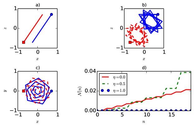
Figure 2: Weak dephasing interaction. Panel a) $\eta=0$, b) $\eta=0.5$, c) $\eta=1.0$ and we have plotted the time evolution of non-zero Bloch vector components. Panel d) plots the measure for non-Markovianity for fixed pair of initial states for the used three values $\eta$. Initial states in all figures are $\vec{r}_{1}=\frac{1}{\sqrt{2}}(1,0,1)^{T}$ and $\vec{r}_{2}=-\vec{r}_{1}$ expressed in terms of the Bloch vector. Parameters of the environment are $A=0$ and $\delta\omega=9\sigma$. Parameters for the interaction are $\Delta n=0.009$ and $\delta t=0.014\frac{2\pi}{\delta\omega\Delta n}$. This gives $\frac{\tilde{\Omega}}{\sigma}\approx 643\gg 1$.

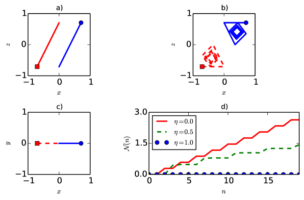
Figure 3: Intermediate dephasing interaction. Panel a) $\eta=0$, b) $\eta=0.5$, c) $\eta=1.0$ and we have plotted the time evolution of non-zero Bloch vector components. Panel d) plots the measure for non-Markovianity for fixed pair of initial states for the used three values $\eta$. Initial states in all figures are $\vec{r}_{1}=\frac{1}{\sqrt{2}}(1,0,1)^{T}$ and $\vec{r}_{2}=-\vec{r}_{1}$ expressed in terms of Bloch vector. Parameters of the environment are $A=0$ and $\delta\omega=9\sigma$. Parameters for the interaction are $\Delta n=0.009$ and $\delta t=2\frac{2\pi}{\delta\omega\Delta n}$. This gives $\frac{\tilde{\Omega}}{\sigma}=4.5\sim 1$.

IV.3 Strong dephasing limit

Let us assume that we have a “flat” population distribution for the initial environmental state. What we mean by this is that, $|\chi(\omega)|^{2}$ stays almost constant for $\omega\in[\omega^{\prime}-{\tilde{\Omega}}/2,\omega^{\prime}+\tilde{\Omega}/2]$, where $\omega^{\prime}\in[0,\infty)$.

Now, this means that the effects of the environment in this limit are generic in the sense, that the global structure of $|\chi(\omega)|^{2}$ does not play a role. This type of environment is usually called ’Markovian’. It is intuitively clear that in this type of situation it is enough to integrate only over a single period of length $\tilde{\Omega}$ in Eq. (14) to a very good approximation. In terms of equations this means

$$\vec{r}(m)= \frac{1}{\tilde{\Omega}}\int_{0}^{\tilde{\Omega}}d\omega M(\omega)^{m}\vec{r}.$$ (30)

Physical idea behind this approximation is that there is no distinguished frequency of the environment because of the flatness of the spectrum. Then all the frequencies in the interval of length $\tilde{\Omega}$ “mix” the state of the reduced system with equal weights, hence it is sufficient to consider only one of these intervals.

In general we have to validate this approximation numerically, but for the special case where $\eta=\frac{1}{2}$ and $A=0$ we can obtain analytical expressions for dynamical map in the strong dephasing limit, which we will do next. It turns out that we will need the condition $\sigma\gg\tilde{\Omega}$ for the analytical calculation but the numerical data shows that already for intermediate dephasing, $\sigma\sim\tilde{\Omega}$, strong dephasing approximation (30) works quite well, see Fig. 4. Dynamics in the intermediate and strong dephasing regime for $\eta=\frac{1}{2}$ is plotted in panel b) of Figs. 2 and 3.

We now give a more detailed proof of Eq. (30) for $\eta=\frac{1}{2}$ and $A=0$. Let $\eta=\frac{1}{2}$ and $|\chi(\omega)|^{2}=\frac{1}{\sqrt{2\pi}\sigma}e^{-\frac{(\omega-\mu)^{2}}{2\sigma^{2}}}$. We assume that $\tilde{\Omega}\ll\sigma$, which means that the spectral distribution varies in much larger scale than the integral kernel $M(\omega)$, which takes the following form

$$M(\omega)=\begin{pmatrix}0&-\sin(\Delta n\delta t\omega)&\cos(\Delta n\delta t\omega)\\ 0&-\cos(\Delta n\delta t\omega)&-\sin(\Delta n\delta t\omega)\\ 1&0&0\end{pmatrix}.$$ (31)

We decompose the interval $\mathbb{R}_{+}=[0,\infty)$ as $\bigcup_{k\in\mathbb{N}\setminus\{0\}}\tilde{\Omega}_{k}$, where $\tilde{\Omega}_{k}=[\tilde{\Omega}\cdot(k-1),\tilde{\Omega}\cdot k)$. Since $\int_{\Omega_{k}}{\rm d}\omega|\chi(\omega)|^{2}$ is continuous on closed interval $\overline{\tilde{\Omega}_{k}}$ and differentiable on $\tilde{\Omega}_{k}$, mean value theorem states that we can always find $\omega_{k}\in\tilde{\Omega}_{k}$ such that

$$|\chi(\omega_{k})|^{2}\tilde{\Omega}=\int_{\tilde{\Omega}_{k}}{\rm d}\omega|\chi(\omega)|^{2}.$$ (32)

As an approximation we choose the midpoint of each interval, $\omega_{k}=\tilde{\Omega}\cdot k+\frac{\tilde{\Omega}}{2}$, then

$$\sum_{k\in\mathbb{N}\setminus\{0\}}|\chi(\omega_{k})|^{2}\tilde{\Omega}= \vartheta_{3}(\pi(\frac{1}{2}-\mu/\tilde{\Omega}),e^{-2\pi^{2}\sigma^{2}/\tilde{\Omega}^{2}}),$$ (33)

where $\vartheta_{3}(u,q)$ is Jacobi theta function.

Condition $\tilde{\Omega}\ll\sigma$ allows to do the following approximation

$$\sum_{k}\int_{\tilde{\Omega}_{k}}{\rm d}\omega|\chi(\omega)|^{2}M(\omega)^{m} \approx\sum_{k}|\chi(\omega_{k})|^{2}\int_{\Omega_{k}}{\rm d}\omega M(\omega)^{m}=\sum_{k}|\chi(\omega_{k})|^{2}\tilde{M}(m)$$

$$=\frac{1}{\tilde{\Omega}}\vartheta_{3}(\pi(\frac{1}{2}-\mu/\tilde{\Omega}),e^{-2\pi^{2}\sigma^{2}/\tilde{\Omega}^{2}})\tilde{M}(m),$$ (34)

where $\tilde{M}(m)=\int_{\Omega_{k}}{\rm d}\omega M(\omega)^{m}$ and we used Eq. (33) in the last step. When we take the strong dephasing limit, $\sigma\to\infty$ and use the property $\lim_{q\to 0}\vartheta_{3}(u,q)=1$ of the Jacobi theta function we obtain Eq. (30) Abramowitz and Stegun (1964). Next we will construct the dynamical map in this special case.

IV.4 Dynamical map in strong dephasing limit for $A=0$ and $\eta=\frac{1}{2}$

In the strong dephasing limit for single Gaussian spectral distribution and $\eta=\frac{1}{2}$ we obtain the following analytical form for the dynamical map $\Lambda_{m}=\frac{1}{\tilde{\Omega}}\int_{0}^{\tilde{\Omega}}M(\omega)^{m}$

$$\Lambda_{0}= \mathbb{I}, \Lambda_{1}= \begin{pmatrix}0&0&0\\ 0&0&0\\ 1&0&0\end{pmatrix},$$

$$\Lambda_{2}= \frac{1}{2}\begin{pmatrix}0&0&1\\ 0&1&0\\ 0&0&0\end{pmatrix}, \Lambda_{3}= \frac{1}{2}\begin{pmatrix}1&0&1\\ 0&1&0\\ 0&0&1\end{pmatrix},$$

$$\Lambda_{2m}= \begin{pmatrix}a_{m-2}&0&a_{m-1}\\ 0&b_{m-1}&0\\ a_{m-2}&0&a_{m-2}\end{pmatrix},m\geq 2, \Lambda_{2m-1}= \begin{pmatrix}a_{m-2}&0&a_{m-2}\\ 0&b_{m-2}&0\\ a_{m-3}&0&a_{m-2}\end{pmatrix},m\geq 3.$$ (35)

where

$$a_{k}= \sum_{i=0}^{k}(2i+1)\frac{C(i)}{(-8)^{i}}, b_{k}= \sum_{i=0}^{k}\frac{C(i)}{(-8)^{i}},$$ (36)

$$a_{k}= b_{k}=0,\,k<0, C(k)= \frac{1}{k+1}\binom{2k}{k},\,k\in\mathbb{N}.$$ (37)

$C(k)$ is called a Catalan number. $a_{k}$ and $b_{k}$ have the following limiting behavior

$$\lim_{k\to\infty}b_{k}= (\sqrt{2}-1), \lim_{k\to\infty}a_{k}= 1-\frac{1}{\sqrt{2}}.$$ (38)

Thus the dynamical map takes the following form in the limit of infinite number of steps

$$\Lambda_{m\to\infty}= \begin{pmatrix}1-\frac{1}{\sqrt{2}}&0&1-\frac{1}{\sqrt{2}}\\ 0&\sqrt{2}-1&0\\ 1-\frac{1}{\sqrt{2}}&0&1-\frac{1}{\sqrt{2}}\end{pmatrix}.$$ (39)

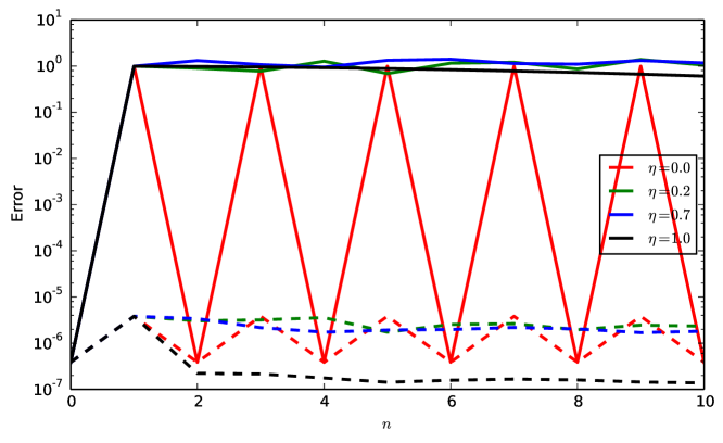
Figure 4: Error of the strong dephasing approximation for few values $\eta$. Error is measured by $d(\Phi^{\rm Q}_{n}-\Lambda_{n})$, eg. the trace distance between the exact ($\Phi^{\rm Q}_{n}$) and approximate ($\Lambda_{n}$) dynamical map. For this calculation we have chosen parameters of the environment as $A=0$ and $\delta\omega=9\sigma$. For interaction we have $\Delta n=0.009$ and the solid lines correspond $\delta t=0.02\frac{2\pi}{\delta\omega\Delta n}$ (weak dephasing) and dashed lines correspond to $\delta t=1.03\frac{2\pi}{\delta\omega\Delta n}$ (intermediate dephsing). These corresponds to the following approximate values $\tilde{\Omega}/\sigma\approx\{450,9\}$ of the quantity measuring the strength of the dephasing.

IV.5 Discussion

The results above show that in a discrete dephasing model for a qubit, the addition of local unitary can induce non-Markovian dynamics even for flat ”Markovian” spectral structure. Local unitary operation can be seen as a periodic control, that dynamically decouples the open system from the environment giving rise to a partial revivals of the populations and coherences in the open system dynamics. Periodicity of this control operation can be seen from the discreteness of the dynamics, i.e., we ”watch” the system only at the integer multiples of the control period. It is also worth noting that the local unitary changes the open system state while the earlier created correlations between the system and environment still persist. The local change in the system state allows then the existing system-environment correlations to be converted back to the increased distinguishability of the system states and backflow of information.

Another effect of the local control, in the case that it does not commute with the dephasing basis, e.g. when $C_{0}=\sigma_{x}$, is that it transforms the open system dynamics from pure dephasing to dissipative. For the case when local control is $C_{1}=\sigma_{z}$, which commutes with the dephasing operator $U_{\delta t}$, the dynamics is pure dephasing type and the action of the local control does not have effect on the non-Markovianity of the dynamics, i.e., non-Markovian dynamics can emerge from the spectral structure only. We also show that the non-Markovianity induced by the local control is generic in the sense that the structure of the environment spectrum does not play a role in the strong dephasing regime. In the special case of Hadamard control $\eta=0.5$ and $A=0$ we were able to derive analytical expression for the dynamical map.

In the following section we study more complicated situation with one dimensional discrete quantum walk. Our findings will be better understood with the help of the physical intuition gained from the present section.

V Open quantum walk

V.1 Quantum walk

Quantum walks are either continuous or discrete time unitary protocols that evolve a quantum state on a Hilbert space that is constructed from the underlying graph where the walk takes place. In this section we will mostly adapt to the notation of Ref. Reitzner et al. (2011).

In this work we limit the discussion to a discrete quantum walks on a line. Hilbert space for the walk is $\mathcal{H}_{W}=\mathcal{H}_{C}\otimes\mathcal{H}_{P}=\mathbb{C}^{2}\otimes\ell^{2}(\mathbb{Z})$. It consists of the coin- and the position space. Unitary operator $W$ evolving the state of the walker over a single step is the following

$$W= (|L\rangle\langle L|\otimes S+|R\rangle\langle R|\otimes S^{\dagger})(C_{H}\otimes\mathbb{I}_{P}),$$ (40)

where $S=\sum_{x}|x-1\rangle\langle x|$ and $C_{H}=C_{\frac{1}{2}}$, see Eq. (12). We choose to focus only on Hadamard walks, meaning that the coin unitary is the Hadamard matrix. The unitary operator $W$ can be diagonalized if we move into a quasi-momentum picture by Fourier transform $|k\rangle=\sum_{x=-\infty}^{\infty}e^{ikx}|x\rangle$, $k\in[-\pi,\pi)$. $k$ is called quasi-momentum since it is periodic. Note that the Fourier- or quasi-momentum basis is not normalizable, but nevertheless very useful when used carefully. The inverse transformation is defined as $|y\rangle=\frac{1}{2\pi}\int_{-\pi}^{\pi}{\rm d}k\,e^{-iky}|k\rangle$.

In this work we always initialize the position of the walker to the origin. In the quasi-momentum picture the unitary operator $W$ acts on an arbitrary state initialized from origin, $|\phi_{0}\rangle=|\phi\rangle\otimes|0\rangle$, as

$$|\phi_{m}\rangle= W^{m}|\phi_{0}\rangle=\int_{-\pi}^{\pi}\frac{{\rm d}k}{2\pi}\,(M_{k})^{m}|\phi\rangle\otimes|k\rangle,$$ (41)

where $M_{k}$ is the following $2\times 2$ matrix

$$M_{k}= \frac{1}{\sqrt{2}}\begin{pmatrix}e^{-ik}&e^{-ik}\\ e^{ik}&-e^{-ik}\end{pmatrix}.$$ (42)

Eigenvalues of $M_{k}$ are $\{e^{-i\nu_{k}},-e^{i\nu_{k}}\}$, where $\nu_{k}$ is defined by

$$\sin k= \sqrt{2}\sin\nu_{k}.$$ (43)

Using the quasi-momentum representation for solving the dynamics and then transforming back to the position representation, we obtain the following expression for a general initial state starting from the origin, $|\psi_{0}\rangle=(c_{L}|L\rangle+c_{R}|R\rangle)\otimes|0\rangle$, and evolving $m$ steps

$$|\psi_{m}\rangle=W^{m}|\psi_{0}\rangle= \sum_{x=-m}^{m}\bigg{[}\big{(}c_{L}A_{L}^{m}(x)+c_{R}A_{R}^{m}(x)\big{)}|L\rangle+\big{(}c_{L}B_{L}^{m}(x)+c_{R}B_{R}^{m}(x)\big{)}|R\rangle\bigg{]}\otimes|x\rangle.$$ (44)

Analytical expressions for the coefficient functions $A_{L}^{m}(x),\,A_{R}^{m}(x),B_{L}^{m}(x),\,B_{R}^{m}(x)$, are obtained most easily from the quasi-momentum picture. They are

$$A_{L}^{m}(x)= \frac{1+(-1)^{m+x}}{2}[\alpha^{m}(x)+\beta^{m}(x)], A_{R}^{m}(x)= \frac{1+(-1)^{m+x}}{2}[\beta^{m}(x)-\gamma^{m}(x)],$$ (45)

$$B_{L}^{m}(x)= \frac{1+(-1)^{m+x}}{2}[\beta^{m}(x)+\gamma^{m}(x)], B_{R}^{m}(x)= \frac{1+(-1)^{m+x}}{2}[\alpha^{m}(x)+\beta^{m}(x)],$$ (46)

where

$$\alpha^{m}(x)= \int_{-\pi}^{\pi}\frac{{\rm d}k}{2\pi}\,e^{i(kx-m\nu_{k})},$$ (47)

$$\beta^{m}(x)= \int_{-\pi}^{\pi}\frac{{\rm d}k}{2\pi}\,\frac{\cos k}{\sqrt{1+\cos\texttwosuperior k}}e^{i(kx-m\nu_{k})},$$ (48)

$$\gamma^{m}(x)= \int_{-\pi}^{\pi}\frac{{\rm d}k}{2\pi}\,\frac{\sin k}{\sqrt{1+\cos\texttwosuperior k}}e^{i(kx-m\nu_{k})}.$$ (49)

Using the method of stationary phase, asymptotic expressions for Eqs. (45) and (46) may be obtained.

After $m$ number of steps the walker has non-zero probability to be found in positions $-m,-m+2,\cdots,m-2,m$. From this follows that after even number of steps the walker has non-zero probability only at even vertices, similarly for odd number of steps. This property is sometimes called modularity.

V.2 Open quantum walk

We extend the the Hilbert space to take into account the effect of an external environment. The extended Hilbert space is $\mathcal{H}=\mathcal{H}_{C}\otimes\mathcal{H}_{P}\otimes\mathcal{H}_{\mathcal{E}}\equiv\mathcal{H}_{\mathcal{S}}\otimes\mathcal{H}_{\mathcal{E}}$ and now our system consists of the coin and position degrees of freedom.

We couple the coin degrees of freedom to the external environment and the coupling unitary is given by the trivial extension of Eq. (5)

$$U_{\delta t}= \int{\rm d}\omega\sum_{\sigma=L,R}e^{in_{\sigma}\omega\delta t}|\sigma\rangle\langle\sigma|\otimes\mathbb{I}_{P}\otimes|\omega\rangle\langle\omega|.$$ (50)

For simplicity we consider only homogeneous case, meaning that the coupling operator acts identically on each vertex of the graph. The walk operator is extended to act on the enlarged Hilbert space trivially, $W\equiv W\otimes\mathbb{I}_{\mathcal{E}}$.

The dynamical map for the open quantum walk is constructed as usual

$$\Phi_{m}^{W}(\rho_{0})= \text{tr}_{\mathcal{E}}\left\{(U_{\delta t}\cdot W)^{m}\rho_{0}\otimes\chi((U_{\delta t}\cdot W)^{\dagger})^{m}\right\},$$ (51)

where $\chi$ is again initial state for the environment. Remarkably, an analytical expression for the dynamical map can be found.

V.2.1 Quantum dynamical map

Matrix elements of the dynamical map are $[\Phi_{m}^{Q}]_{\sigma^{\prime}\sigma,x^{\prime}x;\tau\tau^{\prime},yy^{\prime}}\equiv\langle\sigma^{\prime},x^{\prime}|\Phi_{m}^{Q}(|\sigma,x\rangle\langle\tau,y|)|\tau^{\prime},y^{\prime}\rangle$. We use the following shorthand notation $[\Phi_{m}^{Q}]_{\sigma^{\prime}\sigma,x^{\prime};\tau\tau^{\prime},y^{\prime}}\equiv[\Phi_{m}^{Q}]_{\sigma^{\prime}\sigma,x^{\prime}0;\tau\tau^{\prime},0y^{\prime}}$. Matrix elements can be written explicitly by using the definition of the quantum walk

$$[\Phi_{n}^{Q}]_{\sigma^{\prime}\sigma,x^{\prime};\tau\tau^{\prime},y^{\prime}}= \int{\rm d}\omega\,|\chi(\omega)|^{2}\sum_{\begin{subarray}{c}k_{n},\cdots,k_{1}=\{L,R\}\\ l_{n},\cdots,l_{1}=\{L,R\}\end{subarray}}e^{\left[i\omega\delta t\sum_{s,v=1}^{n}(n_{k_{s}}-n_{l_{v}})\right]}$$

$$\times\left(c_{k_{n},k_{n-1}}\cdots c_{k_{1},\sigma}\right)\left(\bar{c}_{l_{n},l_{n-1}}\cdots\bar{c}_{l_{1},\tau}\right)\langle\sigma^{\prime}|k_{n}\rangle\langle l_{n}|\tau^{\prime}\rangle$$

$$\langle x^{\prime}|K_{k_{n}}\cdots K_{k_{1}}|0\rangle\langle 0|K_{l_{1}}^{\dagger}\cdots K_{l_{n}}^{\dagger}|y^{\prime}\rangle,$$ (52)

where $K_{L}=S$, $K_{R}=S^{\dagger}$ and $c_{\sigma,\sigma^{\prime}}=\langle\sigma|C_{H}|\sigma^{\prime}\rangle$.

Each non-zero inner product $\langle x^{\prime}|K_{k_{n}}\cdots K_{k_{1}}|0\rangle$ in Eq. (V.2.1) corresponds to a path $0\to x^{\prime}$ in a $n$-level binary tree. Each path $0\to x$ has $N_{L}^{n}(x)=\frac{n-x}{2}$ and $N_{R}^{n}(x)=\frac{n+x}{2}$ left and right turns. This allows to write the exponential part of Eq. (V.2.1) as

$$e^{\left[i\omega\delta t\sum_{s,v=1}^{n}(n_{k_{s}}-n_{l_{v}})\right]}= e^{i\omega\delta t\Delta n(y^{\prime}-x^{\prime})},$$ (53)

where $\Delta n=n_{L}-n_{R}$, since left and right turns each contribute to the sum in total $N_{L}(x)$ and $N_{R}(n)$ times the term $n_{L}$ and $n_{R}$, respectively. Then by suppressing the explicit matrix products we can write the matrix element as

$$[\Phi_{n}^{Q}]_{\sigma^{\prime}\sigma,x^{\prime};\tau\tau^{\prime},y^{\prime}}= \int{\rm d}\omega\,|\chi(\omega)|^{2}e^{i\omega\delta t\Delta n(y^{\prime}-x^{\prime})}\langle\sigma^{\prime},x^{\prime}|W^{n}|\sigma,0\rangle\langle\tau,0|(W^{\dagger})^{n}|\tau^{\prime},y^{\prime}\rangle.$$ (54)

This shows, that the coupling of the coin degrees of freedom to the external environment has an effect only on the coherences between different sites. It does not have any effect on the position distribution or to the propagation speed.

V.2.2 Strong dephasing limit

In the strong dephasing limit the state of the quantum system is block diagonal since the coherences between any two different sites in the lattice are destroyed. This means that the state of the quantum walker can be written as

$$\rho_{m}= \bigoplus_{x\in[-m,m]}\tilde{\rho}^{m}(x),$$ (55)

where $\tilde{\rho}^{m}(x)=\sum_{\sigma,\sigma^{\prime}=\{L,R\}}\tilde{\rho}^{m}_{\sigma,\sigma^{\prime}}(x)|\sigma,x\rangle\langle\sigma^{\prime},x|$. Eigenvalues of a self-adjoint $2\times 2$ matrix $\begin{pmatrix}a&b\\ b^{*}&c\end{pmatrix}$ are $\lambda_{\pm}=\frac{1}{2}\left(a+b\pm\sqrt{(a-c)^{2}+4|b|^{2}}\right)$.

Pure initial state $|\psi_{0}\rangle=c_{L}|L,0\rangle+c_{R}|R,0\rangle$ evolves in $m$-steps in the strong dephasing limit into $\Phi_{m}^{W}(|\psi_{0}\rangle\langle\psi_{0}|)$. Expression for block $x$ is

$$\langle x|\Phi_{m}^{W}(|\psi_{0}\rangle\langle\psi_{0}|)|x\rangle=\langle x|W^{m}|\psi_{0}\rangle\langle\psi_{0}|(W^{\dagger})^{m}|x\rangle\equiv\tilde{\rho}_{\psi_{0}}(x).$$ (56)

Characterization of non-Markovianity becomes now more feasible, since we need to diagonalize at the $m$th step $2m+1$ $2\times 2$ self-adjoint matrices, instead of $m^{2}$ valued matrix. Analytical expression by using Eqs. (44),(45),(46) could be obtained, but in this work it we do not analyze it further.

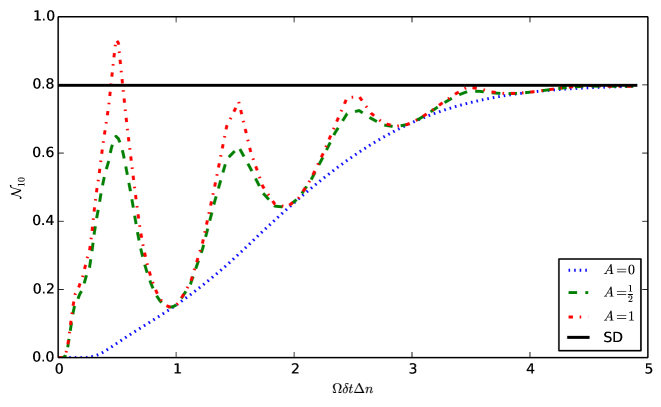
Figure 5: Non-Markovianity of the Quantum walk after ten time steps, $\mathcal{N}_{10}$. Parameter $A$ controls the structure of the environment spectrum. See text for other parameter values. Non-Markovianity is plotted as a function of the dimensionless interaction time of each dephasing unit. As $\delta t\Omega\Delta n$ increases the dephasing effect of each $U_{\delta t}$ becomes stronger and the solid black line corresponds to the strong dephasing limit.

V.2.3 Non-Markovianity of the open quantum walk

We choose the initial state pair for the walk to be $|L\rangle|0\rangle$ and $|R\rangle|0\rangle$ for simplicity. Parameters of the environment are $\delta\omega=9\sigma$, $\Delta n=0.009$, and we vary the value of parameter $A$ which controls the structure of the environment. Non-Markovianity as a function of the dimensionless parameter $\delta t\Omega\Delta n$ is plotted in Fig. 5, where $\Omega=\frac{\delta\omega}{2\pi}$.

We can see that the measure for non-Markovianity is periodic when we increase $\delta t$ which gives the duration of the dephasing step. Remarkably, for a specific values of $\delta t$ the structure of the environment is irrelevant, i.e., for specific duration of dephasing, the quantity of memory effects remain the same irrespective of the structure of the environment. The periodicity of the measure is related to the separation of the peaks of the environment spectrum in the sense that $\mathcal{N}|_{A=0}=\mathcal{N}|_{A=a}$ when $\delta t=m\frac{2\pi}{\delta\omega\Delta n}$. It is also very interesting to note that for strong dephasing limit, the value of non-Markovianity approaches a constant value which is again independent of the structure of the environment which resembles the simple discrete qubit dynamics case. However, before the strong dephasing limit when $\delta t$ has small or intermediate value, non-Markovianity has two sources: the local unitary and the environmental structure. For $A=0$, the non-Markovianity originates from the coin flipping only (local unitary) while for other presented values of $A$, the structure of the environment gives additional contribution to the quantity of the memory effects.

VI Summary

We have analyzed in detail two different models for discrete open quantum system dynamics: a simple qubit dynamics with dephasing and more elaborate full open quantum walk model. The results show that the addition of local unitary operation can dramatically change the nature of the open system dynamics and in particular the appearance of memory effects. We have discussed how memory effects generated within our models can become generic in the sense that the structure of the environment spectrum does not play a role – the amount of memory effects is independent of the form of the spectra – and non-Markovianity is solely induced by local unitary operation in these cases. The considered models and observed phenomena give rise to approximation schemes which simplify the description of the dynamics considerably that may prove useful for other contexts too. We have also discussed in detail for the first time a model for open quantum walk where memory effects can be introduced and controlled in an experimentally relevant way. The presented open quantum walk is experimentally realizable using linear optics.