Resolving charm and bottom quark masses in precision Higgs boson analyses

Alexey A. Petrov^a,b,c, Stefan Pokorski^d, James D. Wells^b, Zhengkang Zhang^b

^(a)Department of Physics and Astronomy
Wayne State University, Detroit, MI 48201, USA
^(b)Michigan Center for Theoretical Physics, Department of Physics
University of Michigan, Ann Arbor, MI 48109, USA
^(c)Theoretical Physics Department
Fermilab, P.O. Box 500, Batavia, IL 60510, USA
^(d)Institute of Theoretical Physics
University of Warsaw, Pasteura 5, 02-093 Warsaw, Poland

Masses of the charm and bottom quarks are important inputs to precision calculations of Higgs boson observables, such as its partial widths and branching fractions. They constitute a major source of theory uncertainties that needs to be better understood and reduced in light of future high-precision measurements. Conventionally, Higgs boson observables are calculated in terms of $m_{c}$ and $m_{b}$, whose values are obtained by averaging over many extractions from low-energy data. This approach may ultimately be unsatisfactory, since $m_{c}$ and $m_{b}$ as single numbers hide various sources of uncertainties involved in their extractions some of which call for more careful estimations, and also hide correlations with additional inputs such as $\alpha_{s}$. Aiming at a more detailed understanding of the uncertainties from $m_{c}$ and $m_{b}$ in precision Higgs boson analyses, we present a calculation of Higgs boson observables in terms of low-energy observables, which reveals concrete sources of uncertainties that challenge sub-percent-level calculations of Higgs boson partial widths.

PRESENTED AT

The 7th International Workshop on Charm Physics (CHARM 2015)
Detroit, MI, 18-22 May, 2015

1 Introduction

Precision studies of the Higgs boson are crucial for understanding the origin of electroweak symmetry breaking and searching for new physics beyond the Standard Model (SM). Many well-motivated new physics scenarios predict percent-level deviations from the SM for the Higgs couplings [1]. Accordingly, it is hoped that data at a later stage of the LHC or future facilities will enable (sub)percent-level determinations of the Higgs boson branching fractions and the important partial widths $\Gamma_{H\to Q\overline{Q}}$ ($Q=c,b$) [2, 3, 4, 5]. However, this does not necessarily imply that percent-level new physics effects can be probed. In fact, the power of precision Higgs analyses is limited by theory uncertainties, which are dominated by the parametric uncertainties from the input parameters, especially the charm and bottom quark masses [6, 7, 8]. In terms of the scale-invariant masses in the $\overline{\text{MS}}$ scheme [i.e. solutions to $m_{Q}(\mu)=\mu$], the uncertainty propagation, according to Ref. [7],

$$\frac{\Delta\Gamma_{H\to c\overline{c}}}{\Gamma_{H\to c\overline{c}}}\simeq\frac{\Delta m_{c}(m_{c})}{10~{}\text{MeV}}\times 2.1\%,\quad\frac{\Delta\Gamma_{H\to b\overline{b}}}{\Gamma_{H\to b\overline{b}}}\simeq\frac{\Delta m_{b}(m_{b})}{10~{}\text{MeV}}\times 0.56\%,$$ (1)

indicates that this parametric uncertainty is at the level of a few percent at present, if the input quark masses are taken from the PDG particle listings [10],

$$m_{c}(m_{c})=1.275(25)\text{ GeV},\quad m_{b}(m_{b})=4.18(3)\text{ GeV}.$$ (2)

Note also that $\Delta\Gamma_{H\to b\overline{b}}$ propagates into the calculations of all branching fractions since $b\overline{b}$ is the dominant decay channel of the SM Higgs boson. In light of the projected experimental precision on the Higgs observables, it is thus highly desirable to have a detailed understanding of this dominant theory uncertainty, and hence the improvements needed. In particular, instead of treating $m_{c}$ and $m_{b}$ as single numbers to be read from the PDG, we will make an initial attempt to incorporate the extraction of $m_{c}$, $m_{b}$ from low-energy experiments into precision Higgs analyses. As a result, the vague notion of “uncertainties from quark masses” will be decomposed into concrete sources, some of which represent a serious challenge that calls for further investigation of the low-energy observables. Further details of this work can be found in Ref. [11].

2 A global approach to precision Higgs analyses

A conventional approach to precision Higgs analyses is to regard $m_{c}$ and $m_{b}$ as input “observables”, namely to put them on the same footings as $m_{Z}$ and $m_{H}$. As such they are assigned “experimental” central values and error bars, as in Eq. (2). However, unlike $m_{Z}$ and $m_{H}$, quark masses are not well-defined observables due to confinement. Instead, they are just parameters in the SM Lagrangian. Their values are extracted from the true observables whose theory predictions depend on them. In fact, the PDG quark masses quoted in Eq. (2) are obtained by averaging over many results in the literature, which are extracted from a variety of observables. Much information is hidden by this averaging procedure, making the conventional approach of using the numbers in Eq. (2) unsatisfactory in several aspects. First, the averaging unrealistically assumes no correlations among the various quark masses extractions, some of which use similar data and/or methods. Second, there are correlations between $m_{Q}$ and $\alpha_{s}$ because $\alpha_{s}$ enters the quark masses extractions as an input, but such correlations are not retained in Eq. (2). $m_{Q}$ and $\alpha_{s}$ are then treated as independent inputs when the Higgs observables are calculated, which is strictly speaking incorrect. Furthermore, the meaning of the error bars in Eq. (2) is obscure. They contain not only various experimental and theoretical uncertainties associated with many different observables, but also a self-described inflation of uncertainties by the PDG (see the “Quark masses” review in Ref. [10]). The latter is introduced to account for possibly underestimated uncertainties in some of the reported quark masses in the literature. The problem of uncertainty underestimation was first noticed in Ref. [12], and its impact on precision Higgs analyses will be discussed below.

These unsatisfactory aspects of the conventional approach can in principle be eliminated if we include only true observables $\{\widehat{O}_{i}^{\text{}}\}$ in the $\chi^{2}$ fit, where the $\chi^{2}$ function

$$\chi^{2}=\sum_{ij}\biggl{[}\widehat{O}_{i}^{\text{th}}(\{\mathcal{I}_{k}\})-\widehat{O}_{i}^{\text{expt}}\biggr{]}V^{-1}_{ij}\biggl{[}\widehat{O}_{j}^{\text{th}}(\{\mathcal{I}_{k}\})-\widehat{O}_{j}^{\text{expt}}\biggr{]},$$ (3)

with appropriately determined uncertainties and correlations contained in the covariance matrix $V$, is minimized with respect to the inputs of the calculation $\{\mathcal{I}_{k}\}$. $m_{c}$ and $m_{b}$ are in the set $\{\mathcal{I}_{k}\}$, but not in the set $\{\widehat{O}_{i}^{\text{}}\}$.

For such a fit to be useful, the fit observables $\{\widehat{O}_{i}^{\text{}}\}$ should include those contributing to the extraction of $m_{c}$ and $m_{b}$. Interestingly, while our starting point is precision Higgs analyses, the observables dominating the PDG average of $m_{Q}$ are associated with much lower energy scales $E\sim m_{Q}\ll m_{H}$. They include, for example, low [12, 13, 14, 15, 16] and high [17, 18, 19, 20] moments of $e^{+}e^{-}\to Q\overline{Q}$ inclusive cross section, defined by

$${\cal M}_{n}^{Q}\equiv\int\frac{\mathrm{d}s}{s^{n+1}}R_{Q}(s),\quad\text{where}\,\,R_{Q}\equiv\frac{\sigma(e^{+}e^{-}\to Q\overline{Q}X)}{\sigma(e^{+}e^{-}\to\mu^{+}\mu^{-})},$$ (4)

variants of these moments [21, 22], and moments of lepton energy and hadron mass distributions of semileptonic $B$ decay [23, 24, 25].

As a result, we are led to the following picture:

$$\begin{Bmatrix}\widehat{O}_{1}^{\text{low}}(m_{c},m_{b},\alpha_{s},\dots)\\[2.15277pt] \widehat{O}_{2}^{\text{low}}(m_{c},m_{b},\alpha_{s},\dots)\\[2.15277pt] \widehat{O}_{3}^{\text{low}}(m_{c},m_{b},\alpha_{s},\dots)\\[2.15277pt] \vdots\end{Bmatrix}\Leftarrow\begin{Bmatrix}\text{\text@underline{Inputs}}\\ m_{c}\\ m_{b}\\ \alpha_{s}\\ \vdots\end{Bmatrix}\Rightarrow\begin{Bmatrix}\widehat{O}_{1}^{\text{Higgs}}(m_{c},m_{b},\alpha_{s},\dots)\\[2.15277pt] \widehat{O}_{2}^{\text{Higgs}}(m_{c},m_{b},\alpha_{s},\dots)\\[2.15277pt] \widehat{O}_{3}^{\text{Higgs}}(m_{c},m_{b},\alpha_{s},\dots)\\[2.15277pt] \vdots\end{Bmatrix}.$$ (5)

The low-energy observables $\{\widehat{O}_{i}^{\text{low}}\}$ play an important role in precision Higgs analyses, because they are sensitive to the same set of inputs as the Higgs observables $\{\widehat{O}_{i}^{\text{Higgs}}\}$. The role of low-energy observables is not obvious in the conventional approach, where a large amount of information from $\{\widehat{O}_{i}^{\text{low}}\}$ has been highly processed into just two numbers $m_{c}$ and $m_{b}$. As we strive for higher-precision calculations, this information should be resolved, and the low-energy observables should be more directly engaged. In this way it is in principle straightforward to include correlations among the observables, and retain the correct $\alpha_{s}$ dependence in each observable. We propose this global approach as a long-term goal for the precision Higgs analysis program, which will become more relevant as experimental precisions on $\{\widehat{O}_{i}^{\text{Higgs}}\}$ improve over time, for both rigorous tests of the SM and fits to SM extensions. The observables set can also be enlarged to include precision electroweak observables (e.g. $Z$-pole observables, $m_{W}$, and LEP2 data) to make the global approach even more powerful.

3 Anatomy of theory uncertainties in $\Gamma_{H\to c\overline{c}}$, $\Gamma_{H\to b\overline{b}}$

To assess the theory uncertainties in calculating $\{\widehat{O}_{i}^{\text{Higgs}}\}$ without performing a full-fledged $\chi^{2}$ fit, in particular the uncertainties from our imprecise knowledge of $m_{c}$ and $m_{b}$, it is helpful to pick out two low-energy observables from the set $\{\widehat{O}_{i}^{\text{low}}\}$, and eliminate $m_{c}$ and $m_{b}$ in favor of them in the functions $\widehat{O}_{i}^{\text{Higgs}}(m_{c},m_{b},\alpha_{s},\dots)$. We will choose ${\cal M}_{1}^{c}$ and ${\cal M}_{2}^{b}$, defined in Eq. (4), as the two low-energy observables, motivated by the simplicity of their calculations and the small quoted uncertainties for $m_{c}$ and $m_{b}$ extracted from them. These moments can be calculated by the method of relativistic QCD sum rules [26] (see e.g. Refs. [27, 28] for reviews), which relate them to the vector current correlators:

$${\cal M}_{n}^{Q}=\frac{12\pi^{2}}{n!}\left(\frac{\mathrm{d}}{\mathrm{d}q^{2}}\right)^{n}\Pi_{Q}(q^{2})\biggr{|}_{q^{2}=0},$$ (6)

where

$$(q^{2}g_{\mu\nu}-q_{\mu}q_{\nu})\Pi_{Q}(q^{2})=-i\int\mathrm{d}^{4}x\,e^{iq\cdot x}\langle 0|Tj_{\mu}(x)j_{\nu}^{\dagger}(0)|0\rangle.$$ (7)

$j_{\mu}$ is the electromagnetic current of the quark $Q(=c,b)$. $\Pi_{Q}$ can be calculated via an operator product expansion:

$${\cal M}_{n}^{Q}=\frac{\bigl{(}Q_{Q}/(2/3)\bigr{)}^{2}}{\bigl{(}2m_{Q}(\mu_{m})\bigr{)}^{2n}}\sum_{i,a,b}C_{n,i}^{(a,b)}(n_{f})\biggl{(}\frac{\alpha_{s}(\mu_{\alpha})}{\pi}\biggr{)}^{i}\ln^{a}\frac{m_{Q}(\mu_{m})^{2}}{\mu_{m}^{2}}\ln^{b}\frac{m_{Q}(\mu_{m})^{2}}{\mu_{\alpha}^{2}}+{\cal M}_{n}^{Q,\text{np}},$$ (8)

where $Q_{Q}$ is the electric charge of the quark $Q$, and $C_{n,i}^{(a,b)}$ are functions of the number of active quark flavors $n_{f}$ (4 for ${\cal M}_{n}^{c}$ and 5 for ${\cal M}_{n}^{b}$). The two terms come from perturbation theory and nonperturbative condensates, respectively. Low moments (small $n$) are preferred so that the perturbative part, which has been calculated up to $\mathcal{O}\left(\alpha_{s}^{3}\right)$ [32], dominates. The nonperturbative piece ${\cal M}_{n}^{Q,\text{np}}$ is dominated by the gluon condensate contribution, which has been calculated to next-to-leading order [33], and is nonnegligible only for the charm quark.

The moments ${\cal M}_{n}^{Q}$ are functions of $m_{Q}$ and $\alpha_{s}$, which are renormalized at $\mu_{m}$ and $\mu_{\alpha}$, respectively, in the $\overline{\text{MS}}$ scheme. Physical observables like ${\cal M}_{n}^{Q}$ should not depend on the renormalization scales $\mu_{m}$, $\mu_{\alpha}$. But when they are calculated to finite order in perturbation theory there is residual scale dependence, which is conventionally used to estimate the effects of unknown higher-order terms. It used to be a common practice to set $\mu_{m}=\mu_{\alpha}$, but it is argued in Ref. [12] that the perturbative uncertainty is generally underestimated in this way. Keeping $\mu_{m}$ and $\mu_{\alpha}$ separate, we can invert Eq. (8) to extract $m_{Q}$, as has been done in Refs. [12, 16],

$$m_{c}(m_{c}) = m_{c}(m_{c})\Bigl{[}\alpha_{s}(m_{Z}),{\cal M}_{1}^{c},\mu_{m}^{c},\mu_{\alpha}^{c},{\cal M}_{1}^{c,\text{np}}\Bigr{]},$$ (9)

$$m_{b}(m_{b}) = m_{b}(m_{b})\Bigl{[}\alpha_{s}(m_{Z}),{\cal M}_{2}^{b},\mu_{m}^{b},\mu_{\alpha}^{b}\Bigr{]}.$$ (10)

Here we have assumed the input $\alpha_{s}$ is at the scale $m_{Z}$, from which $\alpha_{s}(\mu_{\alpha})$ can be derived by the renormalization group (RG) equations [34]. Also, RG equations allow us to convert the extracted $m_{Q}(\mu_{m})$ to $m_{Q}(m_{Q})$. It is clear that the quark masses depend not only on the low-energy observables ${\cal M}_{n}^{Q}$, but also on $\alpha_{s}(m_{Z})$ and the renormalization scales in the calculation of ${\cal M}_{n}^{Q}$. All this dependence is retained in Eqs. (9) and (10), and is eventually propagated into the calculated Higgs observables in $\{\widehat{O}_{i}^{\text{Higgs}}\}$. We will focus on the partial widths $\Gamma_{H\to c\overline{c}}$, $\Gamma_{H\to b\overline{b}}$ in the following. Neglecting correlations between $m_{c}$ and ${\cal M}_{1}^{c,\text{np}}$ (which is justified given the large uncertainties in ${\cal M}_{1}^{c,\text{np}}$, see Ref. [11]), we have

$$\Gamma_{H\to c\overline{c}} = \Gamma_{H\to c\overline{c}}\Bigl{[}\{\widehat{O}_{k}^{\text{in}}\},m_{c}(m_{c}),\mu_{H}^{c}\Bigr{]}$$ (11)

$$= \Gamma_{H\to c\overline{c}}\Bigl{[}\{\widehat{O}_{k}^{\text{in}}\},{\cal M}_{1}^{c},\mu_{m}^{c},\mu_{\alpha}^{c},\mu_{H}^{c},{\cal M}_{1}^{c,\text{np}}\Bigr{]},$$

$$\Gamma_{H\to b\overline{b}} = \Gamma_{H\to b\overline{b}}\Bigl{[}\{\widehat{O}_{k}^{\text{in}}\},m_{b}(m_{b}),\mu_{H}^{b}\Bigr{]}$$ (12)

$$= \Gamma_{H\to b\overline{b}}\Bigl{[}\{\widehat{O}_{k}^{\text{in}}\},{\cal M}_{2}^{b},\mu_{m}^{b},\mu_{\alpha}^{b},\mu_{H}^{b}\Bigr{]},$$

where $\{\widehat{O}_{k}^{\text{in}}\}\equiv\{m_{Z},\;G_{F},\;\alpha(m_{Z}),\;m_{t},\;\alpha_{s}(m_{Z}),\;m_{H}\}$ is the input observables set familiar in precision electroweak analyses. $\mu_{H}^{Q}\sim\mathcal{O}\left(m_{H}\right)$ collectively denotes the renormalization scales chosen in the calculations of $\Gamma_{H\to c\overline{c}}$ and $\Gamma_{H\to b\overline{b}}$, and should not be confused with $\mu_{m}^{Q},\mu_{\alpha}^{Q}\sim\mathcal{O}\left(2m_{Q}\right)$. Note that the $\alpha_{s}(m_{Z})$ dependence has changed in the second equalities in Eqs. (11) and (12) to account for the correlations between $\alpha_{s}$ and $m_{Q}$ reflected in Eqs. (9) and (10).

Eqs. (11) and (12) show the decomposition of the theory uncertainties in $\Gamma_{H\to c\overline{c}}$, $\Gamma_{H\to b\overline{b}}$. In particular, what people usually refer to as “uncertainties from $m_{c}$ and $m_{b}$” are broken down into concrete sources of uncertainties, the most important ones being the parametric uncertainty from the measurements of the low-energy observables ${\cal M}_{1}^{c}$ and ${\cal M}_{2}^{b}$, and the perturbative uncertainty reflected by the residual scale dependence. While the former is straightforward to quantify and interpret, the latter necessarily involves artificial prescriptions that may lead to bias in its estimation, as we will discuss below. We also note that the parametric uncertainty from $\alpha_{s}(m_{Z})$ is affected by the dependence of the extracted $m_{Q}(m_{Q})$ on $\alpha_{s}(m_{Z})$, and is found to be smaller than the incorrect estimate neglecting this correlation; see Fig. 2 below.

To visualize the perturbative uncertainty from the dependence on $\mu_{m}$, $\mu_{\alpha}$, we fix all the input observables at their experimental central values listed in Ref. [11] and set $\mu_{H}=m_{H}$, and make contour plots for the calculated $\Gamma_{H\to c\overline{c}}$, $\Gamma_{H\to b\overline{b}}$ in the $\mu_{m}$-$\mu_{\alpha}$ plane. These plots, shown in Fig. 1, illustrate the propagation of the scale dependence from the low-energy observables to the Higgs boson partial widths, as the latter are seen to depend on the renormalization scales chosen when calculating the former. The necessity to go beyond $\mu_{m}=\mu_{\alpha}$ is clear since the diagonal does not capture all the scale dependence. To estimate the perturbative uncertainty, a common practice is to vary the renormalization scales within a factor of 2 around a characteristic scale of the process. But this does not directly apply to $\mu_{m}$ and $\mu_{\alpha}$, because the ${\cal M}_{n}^{Q}$ receive contributions from all $\sqrt{s}$; see Eq. (4). Therefore, for illustration we will vary $\mu_{m}$ and $\mu_{\alpha}$ independently within an adjustable range $[\mu_{\rm min},\mu_{\rm max}]$, and plot the estimated perturbative uncertainty as a function of $\mu_{\rm min}$ for a few choices of $\mu_{\rm max}$ in Fig. 2. The leading parametric uncertainties are shown in the same figure for comparison.

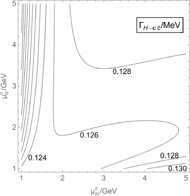
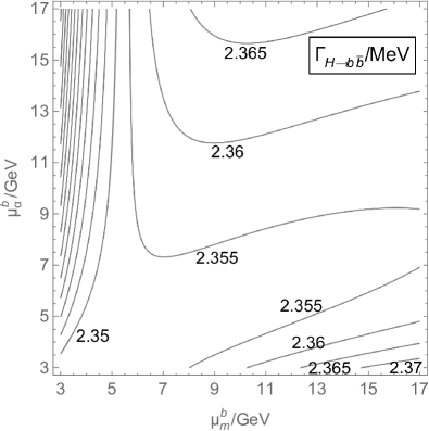
Figure 1: Contours of $\Gamma_{H\to c\overline{c}}$, $\Gamma_{H\to b\overline{b}}$ in MeV in the $\mu_{m}$-$\mu_{\alpha}$ plane. Unlabeled contours represent decreasing values toward the top-left corner in steps of 0.002, 0.005, respectively. The diagonal $\mu_{m}=\mu_{\alpha}$ does not capture all the perturbative uncertainty.

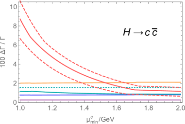
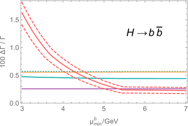
Figure 2: Percent relative uncertainties in $\Gamma_{H\to c\overline{c}}$, $\Gamma_{H\to b\overline{b}}$ as functions of $\mu_{\rm min}$ from various sources: perturbative uncertainty with $\mu_{\rm max}^{c}=4$ GeV, $\mu_{\rm max}^{b}=15$ GeV (red solid) or alternatively $\mu_{\rm max}^{c}=3,5$ GeV, $\mu_{\rm max}^{b}=13,17$ GeV (red dashed), parametric uncertainties from ${\cal M}_{1}^{c}$ or ${\cal M}_{2}^{b}$ (orange), $\alpha_{s}(m_{Z})$ (cyan solid), ${\cal M}_{1}^{c,\text{np}}$ (blue, for $\Gamma_{H\to c\overline{c}}$ only) and $m_{H}$ (purple). The parametric uncertainty from $\alpha_{s}(m_{Z})$ incorrectly calculated assuming no correlation with $m_{Q}$ (cyan dotted) is also shown for comparison. See Ref. [11] for more details.

It is seen from Fig. 2 that the perturbative uncertainty from $\mu_{m}$, $\mu_{\alpha}$ is very sensitive to the somewhat arbitrary choice of $\mu_{\rm min}$, and can dominate the total theory uncertainty for $\Gamma_{H\to c\overline{c}}$, $\Gamma_{H\to b\overline{b}}$ if lower renormalization scales are allowed in the calculations of ${\cal M}_{n}^{Q}$. This represents a serious challenge for higher-precision Higgs boson partial widths calculations, and can be truly overcome only by calculating ${\cal M}_{n}^{Q}$, or equivalently $\bigl{(}\frac{\mathrm{d}}{\mathrm{d}q^{2}}\bigr{)}^{n}\Pi_{Q}(q^{2})\bigr{|}_{q^{2}=0}$ to higher order. Before this calculation is done, ideas on more enlightened prescriptions for the uncertainty estimation may be helpful. Two possibilities, the convergence test [16] and optimal scale setting [35, 36, 37], are discussed in Ref. [11], but both of them are still unsatisfactory at present. It is possible that the actual situation is better in a global $\chi^{2}$ fit incorporating more observables in $\{\widehat{O}_{i}^{\text{low}}\}$, but it remains to investigate other low-energy observables sensitive to $m_{c}$, $m_{b}$ and see if their calculations are plagued by similar scale-setting ambiguities.

In passing we briefly comment on the perturbative uncertainty from $\mu_{H}$, which is usually estimated by varying $\mu_{H}$ from $m_{H}/2$ to $2m_{H}$; see e.g. Ref. [7]. It can be argued that this procedure is incomplete, since the calculations of $\Gamma_{H\to c\overline{c}}$, $\Gamma_{H\to b\overline{b}}$ also involve more than one renormalized parameters, and the renormalization scales chosen for $m_{Q}$ and $\alpha_{s}$ need not be equal. However, we have found that in this case, keeping the scales separate does not significantly increase the estimated uncertainty. Thus, the estimates in the literature with only one scale are expected to be robust.

4 Conclusions

The success of the SM is based on its agreement with data for processes across all accessible energy scales. Charm and bottom quark masses provide a bridge connecting two distinct scales $m_{Q}$ and $m_{H}$. At the next level of precision in testing the Higgs sector of the SM, theory calculations need to be improved to match the projected experimental precision. For a better understanding and a more consistent treatment of the theory uncertainties, it is desirable to resolve the information contained in $m_{c}$ and $m_{b}$ extracted from low-energy data. We have proposed a global approach involving low-energy observables and Higgs observables as a long-term goal for the precision program, and performed a first calculation that connects the two sets of observables. The analysis gives us a more detailed understanding of the “uncertainties from $m_{c}$, $m_{b}$”, and points to future directions for the precision Higgs analysis program.

ACKNOWLEDGEMENTS

A.A.P. is supported in part by the DoE under contract DE-SC0007983, Fermilab’s Intensity Frontier Fellowship and URA Visiting Scholar Award #14-S-23. S.P. is supported by the National Science Center in Poland under the research grants DEC-2012/05/B/ST2/02597 and DEC-2012/04/A/ST2/00099. J.D.W. and Z.Z. are supported in part by the DoE under grant DE-SC0011719.

References

- [1] R. S. Gupta, H. Rzehak and J. D. Wells, Phys. Rev. D 86, 095001 (2012) [arXiv:1206.3560 [hep-ph]].
- [2] D. M. Asner et al., arXiv:1310.0763 [hep-ph].
- [3] M. E. Peskin, arXiv:1312.4974 [hep-ph].
- [4] J. Fan, M. Reece and L. T. Wang, arXiv:1411.1054 [hep-ph].
- [5] M. Ruan, arXiv:1411.5606 [hep-ex].
- [6] A. Denner, S. Heinemeyer, I. Puljak, D. Rebuzzi and M. Spira, Eur. Phys. J. C 71, 1753 (2011) [arXiv:1107.5909 [hep-ph]].
- [7] L. G. Almeida, S. J. Lee, S. Pokorski and J. D. Wells, Phys. Rev. D 89, no. 3, 033006 (2014) [arXiv:1311.6721 [hep-ph]].
- [8] G. P. Lepage, P. B. Mackenzie and M. E. Peskin, arXiv:1404.0319 [hep-ph].
- [9] P. A. Baikov, K. G. Chetyrkin and J. H. Kuhn, Phys. Rev. Lett. 96, 012003 (2006) [hep-ph/0511063].
- [10] K. A. Olive et al. [Particle Data Group Collaboration], Chin. Phys. C 38, 090001 (2014).
- [11] A. A. Petrov, S. Pokorski, J. D. Wells and Z. Zhang, Phys. Rev. D 91, no. 7, 073001 (2015) [arXiv:1501.02803 [hep-ph]].
- [12] B. Dehnadi, A. H. Hoang, V. Mateu and S. M. Zebarjad, JHEP 1309, 103 (2013) [arXiv:1102.2264 [hep-ph]].
- [13] J. H. Kuhn and M. Steinhauser, Nucl. Phys. B 619, 588 (2001) [Nucl. Phys. B 640, 415 (2002)] [hep-ph/0109084].
- [14] J. H. Kuhn, M. Steinhauser and C. Sturm, Nucl. Phys. B 778, 192 (2007) [hep-ph/0702103 [HEP-PH]].
- [15] K. G. Chetyrkin, J. H. Kuhn, A. Maier, P. Maierhofer, P. Marquard, M. Steinhauser and C. Sturm, Phys. Rev. D 80, 074010 (2009) [arXiv:0907.2110 [hep-ph]].
- [16] B. Dehnadi, A. H. Hoang and V. Mateu, arXiv:1504.07638 [hep-ph].
- [17] A. Signer, Phys. Lett. B 672, 333 (2009) [arXiv:0810.1152 [hep-ph]].
- [18] A. Hoang, P. Ruiz-Femenia and M. Stahlhofen, JHEP 1210, 188 (2012) [arXiv:1209.0450 [hep-ph]].
- [19] A. A. Penin and N. Zerf, JHEP 1404, 120 (2014) [arXiv:1401.7035 [hep-ph]].
- [20] M. Beneke, A. Maier, J. Piclum and T. Rauh, Nucl. Phys. B 891, 42 (2015) [arXiv:1411.3132 [hep-ph]].
- [21] S. Bodenstein, J. Bordes, C. A. Dominguez, J. Penarrocha and K. Schilcher, Phys. Rev. D 83, 074014 (2011) [arXiv:1102.3835 [hep-ph]].
- [22] S. Bodenstein, J. Bordes, C. A. Dominguez, J. Penarrocha and K. Schilcher, Phys. Rev. D 85, 034003 (2012) [arXiv:1111.5742 [hep-ph]].
- [23] P. Gambino and C. Schwanda, Phys. Rev. D 89, no. 1, 014022 (2014) [arXiv:1307.4551 [hep-ph]].
- [24] O. Buchmuller and H. Flacher, Phys. Rev. D 73, 073008 (2006) [hep-ph/0507253].
- [25] C. W. Bauer, Z. Ligeti, M. Luke, A. V. Manohar and M. Trott, Phys. Rev. D 70, 094017 (2004) [hep-ph/0408002].
- [26] V. A. Novikov, L. B. Okun, M. A. Shifman, A. I. Vainshtein, M. B. Voloshin and V. I. Zakharov, Phys. Rept. 41, 1 (1978).
- [27] M. A. Shifman, Prog. Theor. Phys. Suppl. 131, 1 (1998) [hep-ph/9802214].
- [28] P. Colangelo and A. Khodjamirian, In *Shifman, M. (ed.): At the frontier of particle physics, vol. 3* 1495-1576 [hep-ph/0010175].
- [29] C. McNeile, C. T. H. Davies, E. Follana, K. Hornbostel and G. P. Lepage, Phys. Rev. D 82, 034512 (2010) [arXiv:1004.4285 [hep-lat]].
- [30] B. Chakraborty et al., Phys. Rev. D 91, no. 5, 054508 (2015) [arXiv:1408.4169 [hep-lat]].
- [31] B. Colquhoun, R. J. Dowdall, C. T. H. Davies, K. Hornbostel and G. P. Lepage, Phys. Rev. D 91, no. 7, 074514 (2015) [arXiv:1408.5768 [hep-lat]].
- [32] A. Maier, P. Maierhofer, P. Marquard and A. V. Smirnov, Nucl. Phys. B 824, 1 (2010) [arXiv:0907.2117 [hep-ph]].
- [33] D. J. Broadhurst, P. A. Baikov, V. A. Ilyin, J. Fleischer, O. V. Tarasov and V. A. Smirnov, Phys. Lett. B 329, 103 (1994) [hep-ph/9403274].
- [34] K. G. Chetyrkin, J. H. Kuhn and M. Steinhauser, Comput. Phys. Commun. 133, 43 (2000) [hep-ph/0004189].
- [35] S. J. Brodsky, G. P. Lepage and P. B. Mackenzie, Phys. Rev. D 28, 228 (1983).
- [36] S. J. Brodsky, M. Mojaza and X. G. Wu, Phys. Rev. D 89, no. 1, 014027 (2014) [arXiv:1304.4631 [hep-ph]].
- [37] A. L. Kataev and S. V. Mikhailov, Phys. Rev. D 91, no. 1, 014007 (2015) [arXiv:1408.0122 [hep-ph]].