On the horizons in a viable vector-tensor theory of gravitation

Abstract

A certain vector-tensor (VT) theory of gravitation was tested in previous papers. In the background universe, the vector field of the theory has a certain energy density, which is appropriate to play the role of vacuum energy (cosmological constant). Moreover, this background and its perturbations may explain the temperature angular power spectrum of the cosmic microwave background (CMB) obtained with WMAP (Wilkinson Map Anisotropy Probe), and other observations, as e.g., the Ia supernova luminosities. The parametrized post-Newtonian limit of the VT theory has been proved to be identical to that of general relativity (GR), and there are no quantum ghosts and classical instabilities. Here, the stationary spherically symmetric solution, in the absence of any matter content, is derived and studied. The metric of this solution is formally identical to that of the Reissner-Nordström-de Sitter solution of GR, but the role of the electrical charge is played by a certain quantity $\Gamma$ depending on both the vector field and the parameters of the VT theory. The black hole and cosmological horizons are discussed. The radius of the VT black hole horizon deviates with respect to that of the Kottler-Schwarzschild-de Sitter radius. Realistic relative deviations depend on $\Gamma$ and reach maximum values close to 30 per cent. For large enough $\Gamma$ values, there is no any black hole horizon, but only a cosmological horizon. The radius of this last horizon is almost independent of the mass source, the vector field components, and the VT parameters. It essentially depends on the cosmological constant value, which has been fixed by using cosmological observational data (CMB anisotropy, galaxy correlations and so on).

Keywords Modified theories of gravity . Spherical symmetry:horizons . Methods: numerical

1 Introduction.

Recently, several vector-tensor (VT) theories –involving a vector field, $A^{\mu}$, and the metric tensor $g^{\mu\nu}$– have been applied to cosmology (Dale, et al., 2009; Dale and Sáez, 2012a); in these theories, the background energy density, $\rho^{A}_{B}$, of the vector field $A^{\mu}$ plays the role of the dark energy (hereafter the subscript $B$ stands for background); for example, in Dale, et al. (2009), where the theory of gravitation considered in this paper was proposed, the equation of state is $P^{A}_{B}=W\rho^{A}_{B}$, where $P^{A}_{B}$ is the pressure due to the field $A^{\mu}$ and $W=-1$; hence, the constant energy $\rho^{A}_{B}$ plays the role of vacuum energy. However, in the theory studied in (Dale and Sáez, 2012a), which might be appropriate to explain the anomalies observed in the angular spectrum of the cosmic microwave background (CMB) for small $\ell$ multipoles, the equation of state is $P^{A}_{B}=W(a)\rho^{A}_{B}$, where $W(a)$ is negative for any value of the scale factor $a$; hence, in this theory, we have a sort of dynamical dark energy different from that associated to the cosmological constant (vacuum energy).

Here, our attention is focused on the theory proposed by Dale, et al. (2009), which was applied to cosmology in Dale and Sáez (2012b) and Dale and Sáez (2014). In this last reference, the VT theory under consideration was proved to be viable in the sense that: (i) its post-Newtonian parametrized limit is identical to that of general relativity (GR), and (ii) the theory may simultaneously explain the seven year WMAP data about the CMB temperature anisotropy and the measurements of supernova Ia luminosities. Conclusion (ii) was obtained by using the well-known Bardeen formalism (Bardeen, 1980) to write the evolution equations of the scalar linear perturbations in VT theory, and also to find the initial conditions at high redshift necessary to solve these equations [see Ma and Bertschinger (1995)]. By using these elements, a modified version of the code COSMOMC (Lewis and Bridle, 2002) –based on statistical techniques as the Markov chains – was designed to fit the VT predictions with the observational data mentioned above. A model involving seven free cosmological parameters was used. Results were encouraging (Dale and Sáez, 2014) and the theory deserves attention.

Before writing any field or cosmological equation, let us fix some notation criteria. Our signature is (–,+,+,+). Latin (Greek) indexes run from 1 to 3 (0 to 3).The symbol $\nabla$ ($\partial$) stands for a covariant (partial) derivative. The antisymmetric tensor $F_{\mu\nu}$ is defined by the relation $F_{\mu\nu}=\partial_{\mu}A_{\nu}-\partial_{\nu}A_{\mu}$, in terms of the $A^{\mu}$ vector field. Quantities $R_{\mu\nu}$, $R$, and $g$ are the covariant components of the Ricci tensor, the scalar curvature and the determinant of the matrix $g_{\mu\nu}$ formed by the covariant components of the metric, respectively. The gravitational constant is denoted $G$ and the speed of light $c$. Units are chosen in such a way that $c=G=1$; namely, we use geometrized units. The dimension of any quantity is $L^{n}$, n being an integer number. Length unit is chosen to be the kilometer. Our coordinates are denoted $t$, $r$, $\theta$, and $\phi$. Whatever the quantity $\xi$ may be, $\xi^{\prime}$ stands for a partial derivative with respect to the radial coordinate $r$.

The two VT theories mentioned above correspond to different choices of the parameters $\omega$, $\eta$, $\varepsilon$, and $\gamma$ involved in the action (Will, 1993):

$$I = \int(R/16\pi+\omega A_{\mu}A^{\mu}R+\eta R_{\mu\nu}A^{\mu}A^{\nu}-$$ (1)

$$\varepsilon F_{\mu\nu}F^{\mu\nu}+\gamma\,\nabla_{\nu}A_{\mu}\nabla^{\nu}A^{\mu}+L_{m})\,\sqrt{-g}\,d^{4}x\ ,$$

where the tensor $F_{\mu\nu}$ –defined above– is not the electromagnetic one. The VT theory studied in this paper [see Dale, et al. (2009)] corresponds to the following choice of the free dimensionless parameters involved in action (1): $\omega=0$ and $\eta=\gamma$. In this theory of gravitation, it has been proved that there are no ghosts and unstable modes for $2\varepsilon-\gamma>0$. Moreover, for a homogeneous and isotropic Robertson-Walker background universe, the energy density of the vector field $\rho^{A}_{B}$ has been proved to be

$$\rho^{A}_{B}=\gamma(\nabla\cdot A)_{B}^{2}\ ,$$ (2)

where $(\nabla\cdot A)_{B}=(\nabla_{\mu}A^{\mu})_{B}$. Therefore, constant $\gamma$ must be positive to have $\rho^{A}_{B}>0$. The vector field equations, when applied to Robertson-Walker cosmology, predict a constant value for $(\nabla\cdot A)_{B}$ and, consequently, $\rho^{A}_{B}$ is strictly constant as the vacuum energy density. The viability of VT as a theory of gravitation and its cosmological success require $\gamma$ and $\varepsilon$ parameters satisfying the inequalities $\varepsilon>\frac{\gamma}{2}>0$, but their values cannot be fixed. In this situation, it is worthwhile the design of new applications of the VT theory with the essential aim of fixing $\gamma$ and $\varepsilon$ and any other arbitrary quantity related with our limited knowledge of the $A^{\mu}$ nature and properties, which are being analyzed. Previous outcomes (based on linearity) strongly suggest that the new applications should be nonlinear. On account of these considerations, we have planed the study of various gravitational physical systems as, for example: (a) the black hole horizons of different sizes and their neighborhoods, (b) the cosmological evolution of nonlinear structures (galaxies, clusters, superclusters and so on) by using either approximations or simulations, and (c) binary stellar systems radiating gravitational waves. Here, our attention is focused on the simplest of these problems: the study of the VT horizons of outer (no matter content) spherically symmetric stationary space-times, which are fully characterized by the mass $m$ (no electrical charge and rotation) and the cosmological constant $\Lambda$.

According to its formulation, VT is a theory of pure gravitation. The field $A^{\mu}$ has nothing to do with the potential vector of the electromagnetic field. It does not couple with electrical currents. The U(1) gauge symmetry of Maxwell theory is not required in VT. In other words, VT is a simple and manageable theory of gravitation. The electromagnetic interaction must be described in the standard way.

There are many alternative theories which are being currently studied, some of these theories are only concerned with gravitation; e.g., the so-called $f(R)$ and $f(T)$ theories, where $T$ is the torsion scalar. In these theories the electromagnetic field is treated in the standard way (minimal coupling with the gravitational part of the Lagrangian). In other theories the action is designed to describe both the gravitational and the electromagnetic fields; interesting cases may be found, e.g., in Novello and Perez Bergliaffa (2008), where non-minimal couplings of the electromagnetic field with gravity are proposed. A very promising non-minimal coupling between the electromagnetic field and a $f(R)$ function is applied to cosmology in Bamba and Odintsov (1980), where it is claimed that the theory is viable, and also that inflation and late time acceleration may be simultaneously explained. However, in VT theory, as well as in GR, it must be recognized that inflation is to be produced by additional fields. It is due to the fact that inflation must lead to an isotropic universe, whereas the inflation due to a vector field is expected to be anisotropic. Only a triplet of orthogonal vector fields or N randomly oriented vector fields might produce an isotropic enough expansion (Golovnev et al., 2008), but this is not the case of the VT theory.

In order to explain inflation we could replace $R$ by an appropriated function $f(R)$ in the Lagrangian of the VT theory; in this way, the field $A^{\mu}$ could explain the accelerated late time expansion, whereas the scalar field, associated to $f(R)$ in the Einstein frame, could account for the required inflation; hence, function $f(R)$ would be chosen to achieve a good inflation, without producing late time acceleration, which implies less restrictions to be satisfied by f(R). Nevertheless, we think that before any generalization, the VT theory must be fully developed as a simple viable and manageable gravitation theory, which explains many observations (see above) for arbitrary values of $\epsilon$ and $\gamma$.

This paper is structured as follows: The VT theory is described in Sect. 2, the stationary spherically symmetric solutions of the field equations are found in Sect. 3, the horizons are studied in Sect. 4 and; finally, Section 5 contains a general discussion and a summary of the main conclusions.

2 The VT theory: basic equations.

Variational calculations based on action (1), with $\omega=0$ and $\eta=\gamma$, lead to the following field equations (Dale and Sáez, 2014):

$$G^{\mu\nu}=8\pi\,(T^{\mu\nu}_{m}+T^{\mu\nu}_{VT})+T^{\mu\nu}_{\Lambda}\ ,$$ (3)

where $T^{\mu\nu}_{m}$ is the contribution of matter to the energy-momentum tensor, which have the same form as in GR. Tensor $T^{\mu\nu}_{VT}$ is the contribution due to the $A^{\mu}$ field of the VT theory, whose form is

$$T^{\mu\nu}_{VT} = 2(2\varepsilon-\gamma)[F^{\mu}_{\,\,\,\,\alpha}F^{\nu\alpha}-\frac{1}{4}g^{\mu\nu}F_{\alpha\beta}F^{\alpha\beta}]$$ (4)

$$-2\gamma[\{A^{\alpha}\nabla_{\alpha}(\nabla\cdot A)+\frac{1}{2}(\nabla\cdot A)^{2}\}g^{\mu\nu}$$

$$-A^{\mu}\nabla^{\nu}(\nabla\cdot A)-A^{\nu}\nabla^{\mu}(\nabla\cdot A)]\ ,$$

and $T^{\mu\nu}_{\Lambda}$ also have the same form as in GR; namely,

$$T^{\mu\nu}_{\Lambda}=-\Lambda g^{\mu\nu}\ .$$ (5)

Eqs. (3) are a generalization of the Einstein equations of GR.

Variations of the vector field $A^{\mu}$ in action (1) give

$$2(2\varepsilon-\gamma)\nabla^{\nu}F_{\mu\nu}=J^{{}^{A}}_{\mu}\ ,$$ (6)

where $J^{{}^{A}}_{\mu}=-2\gamma\nabla_{\mu}(\nabla\cdot A)$ plays the role of a fictitious current.

From Eq. (6) one easily gets the relation

$$\nabla^{\mu}J^{{}^{A}}_{\mu}=0\ ,$$ (7)

which may be seen as the conservation law of the fictitious current $J^{{}^{A}}_{\mu}$ defined above.

Since the parameters $\gamma$ and $\epsilon$ are dimensionless, a dimensional analysis of Eqs. (3) and (4) leads to the important conclusion that the dimension of the $A^{\mu}$ components is $L^{0}$. This fact will be important below. By using the chosen units and the relation between the Einstein ($G^{\mu\nu}$) and Ricci ($R^{\mu\nu}$) tensors, Eqs. (3) may be written as follows:

$$R^{\mu}_{\,\,\,\nu}-\frac{1}{2}R\delta^{\mu}_{\,\,\,\nu}\ =\ T^{\mu}_{\,\,\,\nu}\ ,$$ (8)

where $\delta^{\mu}_{\,\,\,\nu}$ is the Kronecker delta, and

$$T^{\mu\nu}=8\pi\,(T^{\mu\nu}_{m}+T^{\mu\nu}_{VT})+T^{\mu\nu}_{\Lambda}\ .$$ (9)

Equation (8) may be easily rewritten in the form:

$$T^{\mu}_{\,\,\,\nu}-\frac{1}{2}T\delta^{\mu}_{\,\,\,\nu}\ =\ R^{\mu}_{\,\,\,\nu}\ ,$$ (10)

$T$ being the scalar $T^{\mu\nu}g_{\mu\nu}$.

We have the basic equations to look for horizons in next Sections.

3 The stationary spherically symmetric case in the VT theory

It is well known that, in the stationary spherically symmetric case, the line element may be written as follows [see e.g., Stephani, et al. (2003)]:

$$ds^{2} = \ -e^{2\alpha(r)}d\tau^{2}+e^{2\beta(r)}dr^{2}$$ (11)

$$+r^{2}(\ d\theta^{2}+sin^{2}\theta\ d\phi^{2})\ ,$$

and, moreover, the covariant components $A_{\mu}$ have the form:

$$A_{\mu}\ \equiv\ [A_{0}(r),A_{1}(r),0,0]\ .$$ (12)

Accordingly, the nonvanishing $F_{\alpha\beta}$ components are

$$F_{10}=-F_{01}=A^{\prime}_{0}\ .$$ (13)

We have the four unknown functions $\alpha(r)$, $\beta(r)$, $A_{0}(r)$, and $A_{1}(r)$ to be found from the field equations of Sect. 2.

Hereafter, it is assumed that the matter tensor $T^{\mu\nu}_{m}$ vanishes and, then, taking into account Eqs. (4), (5), (9), plus Eqs. (11)–(13), one easily get that, in terms of the new dimensionless parameters $\tilde{\gamma}=8\pi\gamma$ and $\tilde{\varepsilon}=8\pi\varepsilon$, the nonvanishing $T^{\mu\nu}$ components are:

$$T^{01} = T^{10}=2\tilde{\gamma}g^{00}g^{11}A_{0}(\nabla\cdot A)^{\prime}\ ,$$ (14)

$$T^{00} = \ g^{00}\{(2\tilde{\varepsilon}-\tilde{\gamma})[g^{00}g^{11}(A^{\prime}_{0})^{2}]$$ (15)

$$-\tilde{\gamma}[2A^{1}(\nabla\cdot A)^{\prime}+(\nabla\cdot A)^{2}]-\Lambda\}\ ,$$

$$T^{11} = \ g^{11}\{(2\tilde{\varepsilon}-\tilde{\gamma})[g^{00}g^{11}(A^{\prime}_{0})^{2}]$$ (16)

$$-\tilde{\gamma}[-2A^{1}(\nabla\cdot A)^{\prime}+(\nabla\cdot A)^{2}]-\Lambda\}\ ,$$

$$T^{22} = \ g^{22}\{(\tilde{\gamma}-2\tilde{\varepsilon})[g^{00}g^{11}(A^{\prime}_{0})^{2}]$$ (17)

$$-\tilde{\gamma}[2A^{1}(\nabla\cdot A)^{\prime}+(\nabla\cdot A)^{2}]-\Lambda\}\ ,$$

$$T^{33} = \ g^{33}\{(\tilde{\gamma}-2\tilde{\varepsilon})[g^{00}g^{11}(A^{\prime}_{0})^{2}]$$ (18)

$$-\tilde{\gamma}[2A^{1}(\nabla\cdot A)^{\prime}+(\nabla\cdot A)^{2}]-\Lambda\}\ .$$

The line element (11) does not depend on time and, consequently, it does not describe a cosmological space-time. This is also valid in GR, where the same line element leads to various metrics as those of Schwarzschild and Kottler-Schwarzschild-de Sitter [see Kottler (1918)]. The region where these solutions are physically significant must be determined in each case; e.g., regions where $g_{00}>0$ must be excluded. In VT, it has been claimed (see above) that the cosmological constant is related with the value of $\nabla\cdot A$ in the background universe, but this value is different from that of the same divergence in the stationary spherically symmetric case; by this reason, in spite of its origin, the cosmological constant is treated as in GR, and it is denoted $\Lambda$.

Let us now look for the stationary spherically symmetric solutions of the VT field equations following various steps.

3.1 First step: proving that $\nabla\cdot A$ is constant

The calculation of $\nabla\cdot A$ may be performed by solving the tensor field equation (8) for $\mu=1$ and $\nu=0$. In this case, since the components $R^{1}_{\,\,\,0}$ and $\delta^{1}_{\,\,\,0}$ vanish, from Eq. (14) one easily obtains: $2\tilde{\gamma}g^{00}g^{11}A_{0}(\nabla\cdot A)^{\prime}=0$; hence, for $\tilde{\gamma}\neq 0$, $g^{00}\neq 0$, $g^{11}\neq 0$, and $A_{0}\neq 0$, it follows that $(\nabla\cdot A)^{\prime}$ vanishes and, consequently, a trivial integration gives

$$\nabla\cdot A=K_{0}\ ,$$ (19)

where $K_{0}$ is an integration constant.

3.2 Second step: deriving the relation $\alpha(r)=-\beta(r)$

The trace $T$ is first calculated by using the $T^{\mu\nu}$ components calculated from Eqs. (14) – (18) and the $g_{\mu\nu}$ metric components. The result is

$$T=-4\tilde{\gamma}[A^{1}(\nabla\cdot A)^{\prime}+(\nabla\cdot A)^{2}]-4\Lambda\ ,$$ (20)

and, then, taking into account this result, Eq. (10), and Eq. (19), one easily get the relation

$$R^{0}_{0}=R^{1}_{1}\ ,$$ (21)

From this equation and the nonvanishing components of the Ricci tensor:

$$R_{00}\ =\ e^{2(\alpha-\beta)}\left[\alpha^{\prime\prime}+(\alpha^{\prime})^{2}-\alpha^{\prime}\beta^{\prime}+2r^{-1}\alpha^{\prime}\right]\ ,$$ (22)

$$R_{11}\ =-\alpha^{\prime\prime}-(\alpha^{\prime})^{2}+\alpha^{\prime}\beta^{\prime}+2r^{-1}\beta^{\prime}\$$ (23)

$$R_{22}\ =\ e^{-2\beta}\left[r(\beta^{\prime}-\alpha^{\prime})-1\right]+1\ ,$$ (24)

$$R_{33}\ =\ sin^{2}\theta\ R_{22}\ ,$$ (25)

the following relation is easily obtained:

$$2r^{-1}(\alpha^{\prime}+\beta^{\prime})\ =\ 0\ .$$ (26)

The same equation is also obtained in GR. After integration, it leads to $\alpha\ =\ -\beta$ [see, e.g., Stephani, et al. (2003)]. Evidently, this relation implies that $g^{00}g^{11}=-1$.

3.3 Third step: calculation of the $A_{0}$ component

Function $A_{0}(r)$ may be calculated by solving Eq. (6) in the stationary spherically symmetric case. Since $\nabla\cdot A$ has been proved to be constant [see Eq. (19)], the vector $J^{{}^{A}}_{\mu}$ vanishes and, consequently, taking into account the relation $2\epsilon\neq\gamma$, which must be satisfied (see Sect. 1), Eq (6) reduces to $\nabla^{\nu}F_{\mu\nu}=0$. Moreover, taking into account Eqs. (12)–(13), the covariant derivative $\nabla^{\nu}F_{\mu\nu}$ may be easily calculated to get

$$A^{\prime\prime}_{0}+2r^{-1}A^{\prime}_{0}\ =\ 0\ .$$ (27)

In terms of the new variable $y=A^{\prime}_{0}$, the last equation reduces to $y^{\prime}+2r^{-1}y=0$. The solution of this equation is $y=A^{\prime}_{0}=-R_{0}/r^{2}$ and, then, a new integration gives

$$A_{0}(r)\ =\ R_{0}r^{-1}+R_{1}\ ,$$ (28)

where $R_{0}$ and $R_{1}$ are integration constants.

3.4 Fourth step: computing metric components

For $\mu=1$ and $\nu=1$, the tensor field equation (10) may be easily written in the form

$$(\tilde{\gamma}-2\tilde{\varepsilon})(A^{\prime}_{0})^{2}-\tilde{\gamma}(\nabla\cdot A)^{2}-\Lambda-T/2=$$

$$e^{2\alpha}\ (-\alpha^{\prime\prime}-2(\alpha^{\prime})^{2}-2r^{-1}\alpha^{\prime})\ ,$$ (29)

where we have taken into account the relation $g^{00}g^{11}=-1$ (see Sect. 3.1), the nonvanishing components of $R_{\mu\nu}$ and $T^{\mu\nu}$ listed in previous Sections, and Eq. (19). In the same way, for $\mu=2$ and $\nu=2$, one finds

$$(2\tilde{\varepsilon}-\tilde{\gamma})(A^{\prime}_{0})^{2}-\tilde{\gamma}(\nabla\cdot A)^{2}-\Lambda-T/2=$$

$$\frac{1}{r^{2}}[e^{2\alpha}(-2\alpha^{\prime}r-1)+1]\ .$$ (30)

Subtracting equations (29) and (30) and multiplying by the factor $e^{-2\alpha}$, the following second order differential equation is obtained:

$$\alpha^{\prime\prime}+2(\alpha^{\prime})^{2}+[r^{-2}+2(\tilde{\gamma}-2\tilde{\varepsilon})(A^{\prime}_{0})^{2}]e^{-2\alpha}-r^{-2}\ =\ 0\ .$$ (31)

This equation can be solved by using the new variable $w\ =\ e^{2\alpha}$. In terms of $w$, Eq. (31) reads as follows:

$$w^{\prime\prime}-2r^{-2}w\ =\ g(r)\ ,$$ (32)

where $g(r)=-2[r^{-2}+2(\tilde{\gamma}-2\tilde{\varepsilon})A^{\prime}_{0})^{2}]$ and $A^{\prime}_{0}=-R_{0}/r^{2}$ (see above in this Section). The general solution of Eq. (32) is $w=w_{h}+w_{p}$, where $w_{h}$ is the general solution of the corresponding homogeneous equation, and $w_{p}$ is a particular solution of the complete inhomogeneous equation. The general solution $w_{h}$ is:

$$w_{h}\ =\ C_{1}w_{1}(r)+C_{2}w_{2}(r)\ =\ C_{1}r^{2}+C_{2}r^{-1}\ ,$$ (33)

$C_{1}$ and $C_{2}$ being integration constants.

In order to obtain a particular solution, $w_{p}$, we may apply the method of parameter variations; according to this method, we must look for a solution of the following form:

$$w_{p}\ =\ u_{1}(r)w_{1}(r)+u_{2}(r)w_{2}(r)\ =$$

$$\ u_{1}(r)r^{2}+u_{2}(r)r^{-1},$$ (34)

where

$$u_{1}(r) = -\int\frac{w_{2}(r)g(r)}{W_{(w_{1},w_{2})}(r)}\ dr$$

$$u_{2}(r) = \int\frac{w_{1}(r)g(r)}{W_{(w_{1},w_{2})}(r)}\ dr\ ,$$ (35)

and $W_{(w_{1},w_{2})}(r)$ is the Wronskian:

$$W_{(w_{1},w_{2})}(r)\ =\ \left|\begin{array}[]{c c}w_{1}(r)&w_{2}(r)\\ w^{\prime}_{1}(r)&w^{\prime}_{2}(r)\end{array}\right|\ =$$ (38)

$$\ w_{1}(r)w^{\prime}_{2}(r)-w^{\prime}_{1}(r)w_{2}(r)\ =\ -3.$$ (39)

So, the particular solution $w_{p}$ takes on the form:

$$w_{p}(r)\ =\ 1-\frac{4}{3}\ (\tilde{\gamma}-2\tilde{\varepsilon})[r^{2}\int r^{-1}(A^{\prime}_{0}(r))^{2}dr-$$

$$r^{-1}\int r^{2}(A^{\prime}_{0}(r))^{2}dr]\ .$$ (40)

Let us now use the explicit form of $A^{\prime}_{0}$ (see above) to easily find

$$w_{p}(r)\ =\ 1+(2\tilde{\varepsilon}-\tilde{\gamma})\ R_{0}^{2}\ r^{-2}\ .$$ (41)

Finally, Eqs. (33) and (41) allow us to write the general form of function $w=e^{2\alpha}$, which directly leads to the metric components

$$g_{00}\ =\ -\big{[}1+C_{1}r^{2}+C_{2}r^{-1}+(2\tilde{\varepsilon}-\tilde{\gamma})R_{0}^{2}\ r^{-2}\big{]}\ ,$$ (42)

and

$$g_{11}\ =-g_{00}^{-1}\ .$$ (43)

3.5 Fifth step: calculation of the $A_{1}$ component

The last step is the integration of Eq. (19) –derived in Sect. 3.1– to get the function $A_{1}(r)$. This equation may be easily rewritten as follows

$$\nabla\cdot A\ =e^{2\alpha}\left[2(\alpha^{\prime}+r^{-1})A_{1}+A^{\prime}_{1}\right]\ =\ K_{0}\ .$$ (44)

This is a linear first order differential equation of the form $h(r)A^{\prime}_{1}=f_{1}(r)A_{1}+K_{0}$, with $h(r)=e^{2\alpha}$ and $f_{1}(r)=-2e^{2\alpha}(\alpha^{\prime}+r^{-1})$. The solution of this equation is:

$$A_{1}(r)=e^{F(r)}\left(K_{1}+\int e^{-F(r)}\frac{K_{0}}{h(r)}\ dr\right)\ ,$$ (45)

where $K_{1}$ is another integration constant, and $F(r)\ =\ \int[f_{1}(r)/h(r)]\ dr$. After performing these integrals, one obtains:

$$A_{1}(r)=\frac{K_{0}r/3+K_{1}r^{-2}}{1+C_{1}r^{2}+C_{2}/r+(2\tilde{\varepsilon}-\tilde{\gamma})R_{0}^{2}\ r^{-2}}\ .$$ (46)

Eqs. (28) and (46) give the vector field $A^{\mu}$, and Eqs. (42) and (43) define the metric of the VT theory in the stationary spherically symmetric case. The resulting metric is a generalization of the Kottler-Schwarzschild-de Sitter one, which is obtained for $C_{1}=-\frac{\Lambda}{3}$, $C_{2}=-2m=-R_{S}$ ($R_{S}$ being the Schwarzschild radius), and $(2\tilde{\varepsilon}-\tilde{\gamma})=0$. In the VT theory we have found a new term $(2\tilde{\varepsilon}-\tilde{\gamma})R_{0}^{2}/r^{2}$, which is positive due to the fact that the relation $2\epsilon-\gamma>0$ must be satisfied [see Sect. 1]. The metric obtained in the framework of the VT theory is similar to the Reissner-Nordström-de Sitter metric (Kayll (1979)), which corresponds to a stationary spherically symmetric charged system in GR. The form of this known metric is

$$g_{00}=-g_{11}^{-1}=-\Big{[}1-\frac{2m}{r}-\frac{\Lambda}{3}r^{2}+\frac{Q^{2}}{r^{2}}\Big{]}\ ,$$ (47)

it involves a positive term proportional to $1/r^{2}$ which depends on the electrical charge $Q$; evidently, in Eqs. (42) and (43), there is also a term of this kind, in which, the role of $Q^{2}$ is played by the constant $(2\tilde{\varepsilon}-\tilde{\gamma})R_{0}^{2}$.

4 Horizons in the VT theory

In the stationary spherically symmetric case, outside the matter distribution, and in the absence of electrical charge, the solution of the VT field equations involves the integration constants $R_{0}$, $R_{1}$, $K_{0}$, $K_{1}$, $C_{1}$, and $C_{2}$. In this situation, the physical system under consideration is fully described by the quantities $m$ and $\Lambda$, whose dimensions –in geometrized units– are $L^{1}$ and $L^{-2}$, respectively. Let us now perform a dimensional analysis to predict the dependence of the parameter $R_{0}$ involved in the metric components in terms of $m$ and $\Lambda$.

The constants $C_{1}$, and $C_{2}$ also appear in GR. Since the dimensions of $g_{\alpha\beta}$ are $L^{0}$, the term $C_{2}/r$ involved in $g_{00}$ is dimensionless and, consequently, the dimension of $C^{2}$ must be $L^{1}$; hence, $C_{2}$ must be a dimensionless number, $\tilde{C}_{2}$, multiplied by $m$; in this case, we have a well known criterion to conclude that $\tilde{C}_{2}=-2$, a number leading to the well known term $-2m/r$. In the same way, the dimensionless character of $C_{1}r^{2}$ leads to the conclusion that the dimension of $C_{1}$ is $L^{-2}$; hence, this term must be the product of a dimensionless constant $\tilde{C}_{1}$ by the factor $\Lambda$. In this case, there are also arguments to conclude that $\tilde{C}_{1}=-1/3$, a number which leads to the well known term $-\Lambda r^{2}/3$ involved in the Kottler-Schwarzschild-de Sitter metric.

A similar analysis may be performed for the constants $R_{0}$ and $R_{1}$; in fact, according to Eq. (28), the dimensionless component $A_{0}$ is the sum of two terms of the form $R_{0}r^{-1}$ and $R_{1}$; hence, the dimensions of $R_{0}$ and $R_{1}$ are $L^{1}$ and $L^{0}$, respectively and, consequently, we conclude that the constant $R_{0}$ must be the product of a dimensionless constant $\tilde{R}_{0}$ by $m$; in this case, we have not any criterion to fix the dimensionless constant $\tilde{R}_{0}$, which keeps arbitrary by the moment. This analysis does not give any information about the dimensionless constant $R_{1}$, but this information is not necessary to look for the horizons, which follows from the fact that –according to Eqs. (42) and (43)– the metric components do not depend on $R_{1}$.

The dimensional analysis in not extended to the component $A_{1}$, since the metric is also independent of the constants $K_{0}$ and $K_{1}$ involved in Eq. (46).

After the above dimensional considerations we can write:

$$A_{0}(r)\ =\ \tilde{R}_{0}m/r\ ,$$ (48)

$$g_{00}\ =\ -g_{11}^{-1}=-\Big{[}1-\frac{\Lambda}{3}r^{2}-\frac{2m}{r}+(2\tilde{\varepsilon}-\tilde{\gamma})\tilde{R}_{0}^{2}\frac{m^{2}}{r^{2}}\Big{]}\ ,$$ (49)

where $\tilde{R}_{0}$ plays the role of a dimensionless arbitrary constants, which should be fixed by studying appropriate nonlinear problems in the framework of the VT theory, as, e.g., the geodesic motion of proof particles close to possible horizons.

In terms of the function $f(r)=-g_{00}(r)$, the horizons are the hypersurfaces $r=r_{h}$ defined by the condition $f(r_{h})=0$. In the regions where the inequality $f(r)>0$ is satisfied, our description of the stationary spherically symmetric space-time is physically consistent. Condition $f(r)<0$ is not compatible with the assumed metric signature.

In the standard $\Lambda$CDM cosmological model of GR, most current observations are explained for values of the vacuum energy density parameter $\Omega_{\Lambda}$ close to $0.73$, which corresponds to $\Lambda\simeq 10^{-46}\ Km^{-2}$. The same value also explains current observations in the framework of the VT theory [see Dale and Sáez (2014)]; hence, the above value of the cosmological constant is hereafter fixed.

The mass $m$ is varied between $10\ M_{\odot}$ and $10^{9}\ M_{\odot}$; so, the masses of different types of black holes are considered. From stellar black holes due to supernova explosions, to supermassive ones located in the galactic central regions.

Once a mass $m$ has been fixed, function $f(r)$ only involves the unknown positive parameter $\Gamma=(2\varepsilon-\gamma)\tilde{R}_{0}^{2}$. For $\Gamma=0$, the metric reduces to the Kottler-Schwarzschild-de Sitter one and, in such a case, there are two horizons, the first (second) one is the black hole (cosmological) horizon, whose radius is hereafter denoted $r_{BH}$ ($r_{C}$). In the region limited by these two horizons, namely, for $r_{BH}<r<r_{C}$, function $f(r)$ is positive and the Kottler-Schwarzschild-de Sitter metric is physically admissible.

Kayll (1979) studied the horizons in the Reissner-Nordström-de Sitter space-time. If the outcomes obtained in that paper are rewritten in our case, by replacing $Q^{2}$ by $(2\tilde{\varepsilon}-\tilde{\gamma})m^{2}\tilde{R}_{0}^{2}$, it is straightforward to conclude that from $\Gamma=0$ to a certain $\Gamma$ value, $\Gamma_{max}$, which is greater than $1/8\pi$ but very close to it, there are both a black hole horizon and a cosmological one; however, for $\Gamma>\Gamma_{max}$, there is an unique horizon which is cosmological. Our calculations have verified all this.

For appropriate $m$ values, the algebraic equation $f(r)=0$ has been numerically solved for $\Gamma=0$ and for many positive $\Gamma$ values. For $\Gamma>1/8\pi$ and whatever $m$ may be, we have found only a root at $r_{C}\simeq 1.73\times 10^{23}\ Km$ (there is no black hole horizon). However, for any $\Gamma<1/8\pi$, apart from the above $r_{C}$ radius for the cosmological horizon, we have also obtained a black hole horizon with a $r_{BH}$ radius depending on both $m$ and $\Gamma$.

Figure 1 corresponds to a mass $m=10\ M_{\odot}$ (stellar black hole). The left panel shows $r_{BH}$ as a function of $\Gamma$ inside the interval [0, $1/8\pi$]. The radius of the black hole horizon decreases as $\Gamma$ separates from the zero value corresponding to the Kottler-Schwarzschild-de Sitter solution of the GR field equations. In the right panel, the relative deviation

$$D=\frac{2[r_{BH}(\Gamma=0)-r_{BH}(\Gamma)]}{r_{BH}(\Gamma=0)+r_{BH}(\Gamma)}$$ (50)

is represented, as a function of $\Gamma$, in the same interval as in the left panel. We see that these deviations reach values close to 30%, which are not very large deviations, but moderate significant ones.

In Figure (2), the mass is $m=10^{9}\ M_{\odot}$ (galactic supermassive black hole) and, consequently, the radius $r_{BH}(\Gamma=0)\simeq 2m$ is greater than in the top panels by a factor of $10^{8}$; nevertheless, this proportionality factor is the same for any $\Gamma$ and, consequently, the form of the curves represented in the left panels of Figs. (1) and (2) are identical. Moreover, the relative deviations $D$ defined in Eq. (50) reach the same values in the right panels of the two Figures, which means that these deviations do not depend on $m$.

5 Conclusions.

This paper has been devoted to the development of the VT theory of gravitation proposed by Dale, et al. (2009). Previous applications of this theory to both the solar system and cosmology have given excellent results (Dale and Sáez, 2014). Here, we have solved the field equations of the VT theory, in the absence of matter and electrical charge, by assuming a stationary spherically symmetric space-time. It has been proved that the resulting solution has the same form as the Reissner-Nordström-de Sitter solution of GR, but the role of the electrical charge is played by a quantity proportional to the source mass $m$. After reaching this conclusion, we have focused our attention on the horizons associated to stellar and massive black holes.

Nojiri and Odintsov (2014) have proved that, in the absence of electrical charge, there are $f(R)$ theories of gravitation leading to Reissner-Nordström-de Sitter space-times, but the authors recognize that -in these theories– the meaning of the quantity playing the role of the electrical charge is not clear.

Since the cosmological constant, $\Lambda$, is fixed by comparisons between predictions of the VT theory and current observations, the cosmological horizon is practically constant. Its radius is almost independent of the mass, $m$, for any realistic black hole. There is always a cosmological horizon whatever the value of the parameter $\Gamma$ defined in Sect. 4 may be.

In the VT theory, we have proved that, for a given mass $m$, the radius of the black hole horizon is smaller than the radius of the Kottler-Schwarzschild-de Sitter black hole having the same mass. The relative deviations between these two radius are small but significant, reaching values close to 30 %. This effect is important since it is similar to the effect due to the black hole rotation in GR, which leads to a horizon radius smaller than that corresponding to $J=0$. For $\Gamma>1/8\pi$ there is no any black hole horizon in the VT theory under consideration.

Various methods have been designed to estimate the mass $m$ and angular momentum $J$ of a black hole from observations. If, in future, the mentioned methods become accurate enough, and the estimated $m$ and $J$ quantities obey the relation predicted by means of the Kerr solution of Einstein equations, the contribution of the vector field to the horizon radius will have to be considered negligible ($\Gamma\simeq 0$); however, if the Kerr relation is not satisfied by the observed values of $m$ and $J$, an appropriate $\Gamma$ value could solve the problem.

Let us finally mention two interesting extensions of this paper: first of all, the motion of test particles in the neighborhood of the above VT black hole deserves attention; so, accretion disks and other phenomena might be studied. Afterward, the stationary axially symmetry line element, plus an appropriate vector field $A^{\mu}$, should be considered to study rotating black holes in the framework of the VT theory; in this way, a relation between $m$ and $J$ could be found, which might be satisfied by accurate future observed values of these quantities.

Acknowledgements This research has been supported by the Spanish Ministry of Economía y Competitividad, MICINN-FEDER project FIS2012-33582

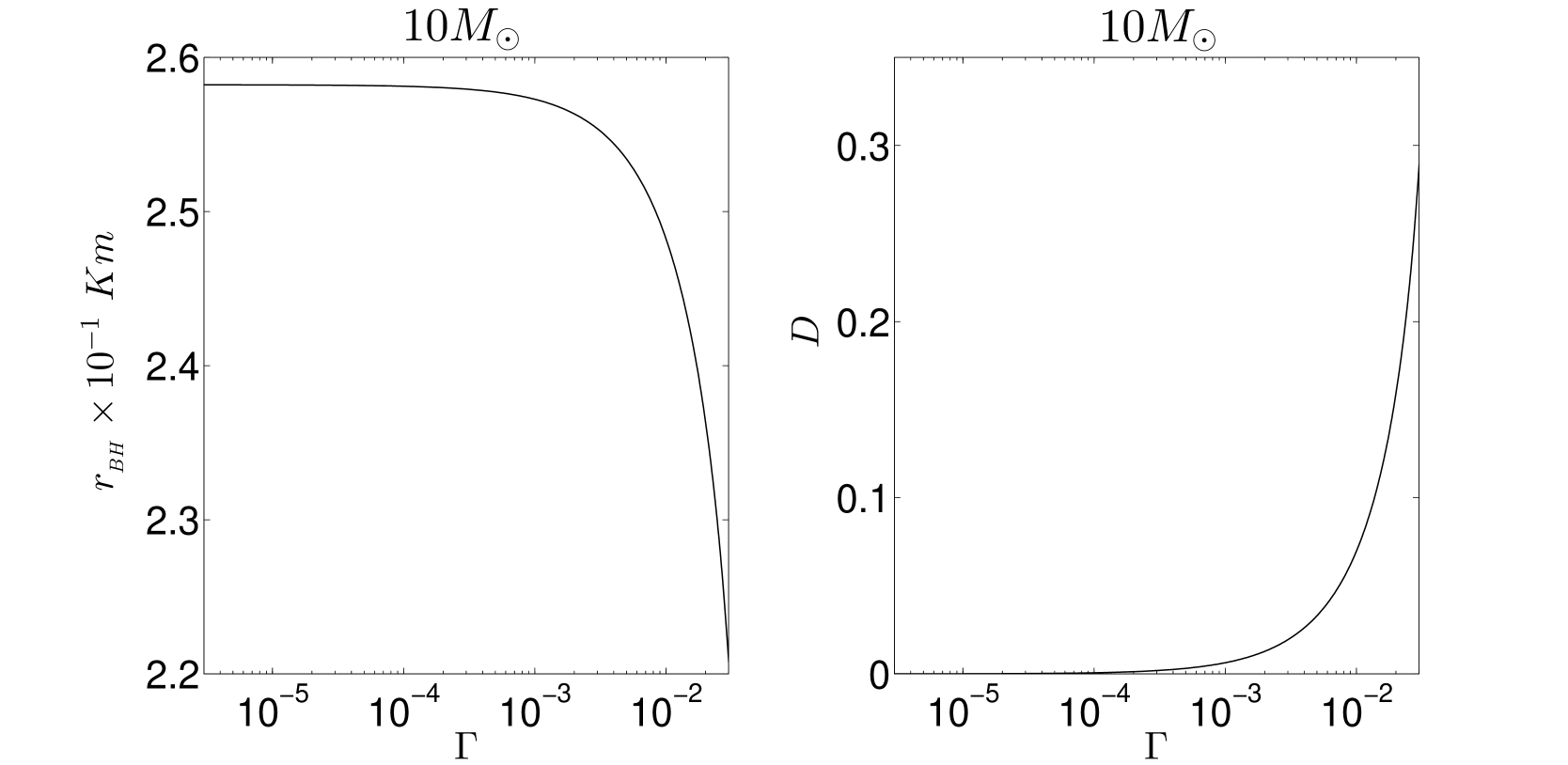
Fig. 1 : Left panel shows the radius $r_{BH}$ of the black hole horizon as a function of $\Gamma$. Right panel represents the relative deviations, $D$, between $r_{BH}(\Gamma=0)$ and $r_{BH}(\Gamma)$, in the $\Gamma$ interval where there is a black hole horizon. In both panels $m=10\ M_{\odot}$

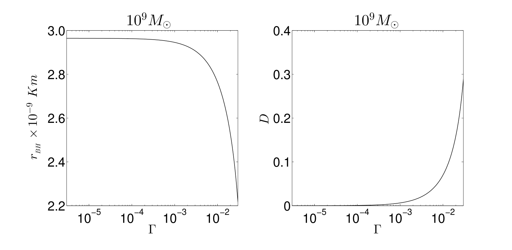
Fig. 2 : Same as in Fig. 1 for $m=10^{9}\ M_{\odot}$

References

- Bamba and Odintsov (1980) Bamba, K., Odintsov, S.D.: J. Cosmol. Astropart. Phys.04, 024 (2008)
- Bardeen (1980) Bardeen, J.M.: Phys. Rev. D22, 1882 (1980)
- Dale, et al. (2009) Dale, R., Morales, J.A., Sáez, D.:(2009). arXiv:0906.2085 [astro-ph]
- Dale and Sáez (2012a) Dale, R., Sáez, D.: Astrophys. Space Sci.337, 439 (2012)
- Dale and Sáez (2012b) Dale, R., Sáez, D.: Phys. Rev. D85, 124047 (2012)
- Dale and Sáez (2014) Dale, R., Sáez, D.: Phys. Rev. D89, 044035 (2014)
- Golovnev et al. (2008) Golovnev, A., Mukhanov, V., Vanchurin, V.: J. Cosmol. Astropart. Phys.06, 009 (2008)
- Kayll (1979) Kayll, L.: Phys. Rev. D19, 421 (1979)
- Kottler (1918) Kottler, F.: Ann. Phys. 361, 401 (1918)
- Lewis and Bridle (2002) Lewis, A., Bridle, S.: Phys. Rev. D66, 103511 (2002)
- Ma and Bertschinger (1995) Ma C.P., Bertschinger, E.: Astrophys. J.455, 7 (1995)