Stable Solitons in Three Dimensional Free Space without the Ground State: Self-Trapped Bose-Einstein Condensates with Spin-Orbit Coupling

Abstract

By means of variational methods and systematic numerical analysis, we demonstrate the existence of metastable solitons in three-dimensional (3D) free space, in the context of binary atomic condensates combining contact self-attraction and spin-orbit coupling, which can be engineered by available experimental techniques. Depending on the relative strength of the intra- and inter-component attraction, the stable solitons feature a semi-vortex or mixed-mode structure. In spite of the fact that the local cubic self-attraction gives rise to the supercritical collapse in 3D, hence the setting produces no true ground state, the solitons are stable against small perturbations, motion, and collisions.

Introduction and model — Solitons result from the balance between dispersion and nonlinearity in diverse physical systems. Stable solitons in one dimension (1D) have been studied extensively in diverse media, most notably nonlinear optics and atomic Bose-Einstein condensates (BECs) books . Multidimensional solitons were also predicted to exist in ferromagnets Cooper , superconductors Babaev , semiconductors semi , BECs Ruostekoski , baryonic matter Alkofer , field theory field , etc. However, creation of 2D and 3D bright solitons is a much more challenging problem than in 1D. The fundamental difficulty is the fact that the ubiquitous cubic local self-attractive nonlinearity gives rise to the critical and supercritical collapse (blowup) in the 2D and 3D geometry, respectively Collapse1 ; Collapse2 ; Collapse3 , which makes all the bright solitons unstable (the self-repulsive nonlinearity supports stable 2D dark solitons in the form of delocalized vortices vortex ). Several theoretical schemes have been elaborated for the stabilization of 2D and 3D solitons. They rely on the use of trapping potentials Dodd ; Morise ; BBB ; Baizakov ; Mihalache05 , sophisticated nonlinear interactions Mihalache02 ; RMP ; Brazil ; Driben , or nonlocal nonlinearity Pohl ; Tikho . However, it is commonly believed that a local cubic self-attraction may never give rise to stable solitons in 3D free space RMP ; dark .

Recently, an essential result Sakaguchi , which helps to resolve a related but easier problem of the stabilization of solitons in 2D free space with local cubic attraction, has been reported in the framework of the model of a binary BEC subject to the action of spin-orbit coupling (SOC) Lin (solitons in 1D SOC models have been predicted too 1d , but their stability is obvious). It was found that the system gives rise to completely stable 2D bright solitons as the ground state (GS). The stabilization is explained by the fact that the linear SOC terms come with a coefficient whose dimension is inverse length. The usual 2D systems without SOC feature a specific scaling invariance, which is closely related to the critical collapse. The scaling invariance makes the family of 2D solitons degenerate (they are called Townes solitons in that case Townes ), with a single value of the norm that does not depend on the soliton’s chemical potential. This norm determines the threshold for the onset of the critical collapse Collapse1 ; Collapse2 . Breaking the scaling invariance by introducing a fixed length scale leads to the stabilization of 2D solitons. This can be achieved by adding trapping potentials Dodd ; Morise ; BBB ; Baizakov ; Mihalache05 or, in the free space, with the help of SOC Sakaguchi , which creates the missing GS by pushing the norm of the 2D solitons below the collapse threshold. A similar mechanism enables the stabilization of 2D spatiotemporal solitons in a planar optical coupler Barcelona , with the coupling’s temporal dispersion Chiang emulating the SOC effect.

It has been previously shown that, besides the stabilization of 2D solitons, the interplay of SOC and intrinsic BEC nonlinearity give rise to a variety of other remarkable phenomena Effect0 . However, the possibility of stabilizing 3D solitons in free space with the help of SOC remained an open question. The fundamental difficulty is that, on the contrary to the 2D situation, the supercritical collapse in 3D has zero threshold, hence the norm cannot take values below the threshold, making the stabilization mechanism outlined above irrelevant in 3D. The present work reveals that, nevertheless, the self-attractive binary SOC condensate can support (meta)stable 3D solitons in free space, in spite of the fact that the setting has no GS at any value of the norm (in other words, the energy is unlimited from below). We find that the SOC-induced modification of the dispersion of the 3D condensate may balance the attractive nonlinearity, creating metastable solitons. In addition to the absence of the GS, another fundamental difference of this mechanism from what is outlined above for 2D is that the stability of the 3D solitons is controlled not by the norm, but rather by their energy.

We follow the usual mean-field approach, defining $\Psi(\mathbf{r})=(\psi_{+},\,\psi_{-})^{T}$ as the condensate wave function, with $\pm$ referring to two pseudo-spin components. Fixing by means of rescaling the atomic mass and Planck’s constant to be $1$, we write the system’s energy as the sum of kinetic, SOC, and interaction terms:

$$E_{\mathrm{tot}} = E_{\mathrm{kin}}+E_{\mathrm{soc}}+E_{\mathrm{int}}\,,$$ (1)

$$E_{\mathrm{kin}} = \frac{1}{2}\int d^{3}r\,\Psi^{{\dagger}}\mathbf{p}^{2}\Psi,~{}E_{\mathrm{soc}}=\lambda\int d^{3}r\,\Psi^{{\dagger}}\left(\mathbf{p}\cdot{\boldsymbol{\sigma}}\right)\Psi,$$

$$E_{\mathrm{int}} = -\frac{g}{2}\int d^{3}r\,\left(|\psi_{+}|^{4}+|\psi_{-}|^{4}+2\eta|\psi_{+}\psi_{-}|^{2}\right)\,,$$

where ${\boldsymbol{\sigma}}=(\sigma_{x},\sigma_{y},\sigma_{z})$ are Pauli matrices, and $\mathbf{p}=-i\nabla$ is the momentum operator. We adopt the 3D isotropic form of the SOC with strength $\lambda$ Anderson . The intra- and inter-component interaction strengths are defined, respectively, as $-g$ and $-\eta g$, with $g>0$ corresponding to the self-attraction, $\eta$ being the relative cross-nonlinearity strength. Below, we fix the nonlinearity strength, by rescaling the wave functions, to $g=1$ and vary the SOC strength $\lambda$, norm $N$, and cross-nonlinearity strength $\eta$.

Dimensional analysis — If $L$ is a characteristic size of the self-trapped condensate, an estimate for the amplitudes of the wave functions with norm $N=\int d^{3}{r}\,\left(|\psi_{+}|^{2}+|\psi_{-}|^{2}\right)$ is $\left(\left|\psi_{\pm}\right|\right)_{\max}\sim\sqrt{N}L^{-3/2}$. Therefore, the three terms in Eq. (1) scale with $L$ as

$$E_{\mathrm{tot}}/N\sim c_{\mathrm{kin}}L^{-2}-c_{\mathrm{soc}}\lambda L^{-1}-\left(c_{\mathrm{int}}^{\mathrm{(self)}}+c_{\mathrm{int}}^{\mathrm{(cross)}}\eta\right)NL^{-3}\,,$$ (2)

with positive coefficients $c_{\mathrm{kin}}$, $c_{\mathrm{soc}}$, and $c_{\mathrm{int}}^{\mathrm{(self/cross)}}$. As shown in Fig. 1, Eq. (2) gives rise to a local minimum of $E_{\mathrm{tot}}(L)$ at finite $L$, provided that

$$0<\lambda N<{c_{\mathrm{kin}}^{2}}/\left[{3\left(c_{\mathrm{int}}^{\mathrm{(self)}}+c_{\mathrm{int}}^{\mathrm{(cross)}}\eta\right)c_{\mathrm{soc}}}\right]\,.$$ (3)

Although this minimum cannot represent the GS (which formally corresponds to $E_{\mathrm{tot}}\rightarrow-\infty$ at $L\rightarrow 0$ in the collapsed state, i.e., the system has no true GS), it corresponds to a self-trapped state stable against small perturbations. Previously, a similar approximate analysis has correctly predicted stable quasi-2D solitons in dipolar BEC Tikho .

Condition (3) suggests that metastable 3D solitons may exist in free space when the SOC term is present, while its strength $\lambda$ is not too large, $N$ and $\eta$ being not too large either. We confirm these expectations below by means of accurate numerical analysis.

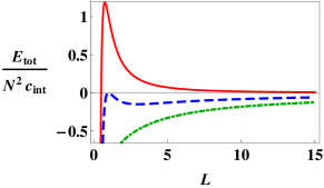
Figure 1: (Color online) $E_{\mathrm{tot}}$ as a function of condensate’s size $L$, as per Eq. (2). The red solid, blue dashed, and green dot-dashed lines represent the energy’s variation when $\lambda=0$, and $\lambda>0$ does or does not satisfy condition (3), respectively.

The Gross-Pitaevskii equation — Energy functional (1) gives rise to the Gross-Pitaevskii equation (GPE) for the spinor wave function,

$$\left[i\frac{\partial}{\partial t}+\frac{1}{2}\nabla^{2}+i\lambda\nabla\cdot{\boldsymbol{\sigma}}\right.$$

$$\left.+g\left(\begin{array}[]{cc}|\psi_{+}|^{2}+\eta|\psi_{-}|^{2}&0\\ 0&|\psi_{-}|^{2}+\eta|\psi_{+}|^{2}\end{array}\right)\right]\Psi=0.$$ (6)

Assuming axial symmetry of the expected self-trapped states (it is the highest symmetry admitted by the SOC Sakaguchi ) and using cylindrical coordinates $(r,z,\phi)$, the stationary wave function with integer vorticity $m\geq 0$ and chemical potential $\mu$ is looked for as

$$\left(\begin{array}[]{c}\psi_{+}\\ \psi_{-}\end{array}\right)=e^{-i\mu t}\left(\begin{array}[]{c}e^{im\phi}\,f_{1}(r,z)\\ e^{i(m+1)\phi}\,f_{2}(r,z)\end{array}\right)\,.\,$$ (7)

Following the terminology introduced for 2D solitons in Ref. Sakaguchi , self-trapped states (7) with $m=0$ are called semi-vortices (SVs), the states with $m\geq 1$ being their excited states. Similar to the 2D system Sakaguchi , our calculations demonstrate that the energy of the SV with $m=0$ is always lowest, therefore we focus on $m=0$.

Due to the up-down symmetry of underlying Hamiltonian (1), degenerate to SV (7) is its flipped counterpart,

$$\left(\begin{array}[]{c}\psi_{+}\\ \psi_{-}\end{array}\right)=e^{-i\mu t}\,\left(\begin{array}[]{c}e^{-i\left(m+1\right)\phi}\,f_{2}^{\ast}(r,z)\\ e^{-im\phi}\,f_{1}^{\ast}(r,z)\end{array}\right)\,,\,$$ (8)

with $\ast$ standing for the complex conjugate. Although the system is axially symmetric, stationary states do not necessarily follow this symmetry. In particular, any superposition of ansätze (7) and (8) breaks the symmetry. Following the nomenclature introduced in Ref. Sakaguchi , we call the state generated by such a superposition a mixed mode (MM). Approximating it by the superposition with mixing angle $\theta$ note ,

$$\begin{split}\psi_{+}&=\left(\cos{\theta}\right)\,f_{1}(r,z)-\left(\sin{\theta}\right)\,f_{2}^{\ast}(r,z)\,e^{-i\phi}\,,\\ \psi_{-}&=\left(\sin{\theta}\right)\,f_{1}^{\ast}(r,z)+\left(\cos{\theta}\right)\,f_{2}(r,z)\,e^{i\phi}\,,\end{split}$$ (9)

straightforward calculation relates its energy to that of the respective SV:

$$E_{\mathrm{MM}} = E_{\mathrm{SV}}+(1-\eta)\sin^{2}{\theta}\cos^{2}{\theta}\,\Delta E\,,$$ (10)

$$\Delta E = 2\pi g\int\!rdr\int\!dz\left(|f_{1}|^{4}+|f_{2}|^{4}-4|f_{1}|^{2}|f_{2}|^{2}\right).$$

Our numerical calculations show that $\Delta E$ is always positive, hence, like in the 2D case Sakaguchi , the SV (MM) has lower energy at $\eta<1$ ($\eta>1$) . This prediction is confirmed below by the full numerical analysis.

Variational analysis — To produce analytical results in a more accurate form than given by Eq. (2), we here adopt the following ansatz for the SV:

$$f_{n}=i^{n-1}\left(A_{n}+iB_{n}z\right)r^{n-1}e^{-\alpha_{n}r^{2}-\beta_{n}z^{2}}\;\;(n=1,2)\,,$$

with real parameters $A_{n},B_{n}$, and $\alpha_{n}>0$, $\beta_{n}>0$. The substitution of this ansatz into expression (1) for the full energy and minimizing it with respect to the free parameters produces algebraic equations which can be readily solved numerically. Stable solitons correspond to finite values of $\alpha_{n}$ and $\beta_{n}$, while $\alpha_{n},\beta_{n}\rightarrow 0$ (spreading) and $\alpha_{n},\beta_{n}\rightarrow\infty$ (collapsing) indicate that no solitons exist. Results of the calculations are summarized in Fig. 2, in which the stable 3D solitons are predicted to exist in the shaded areas. We thus conclude that the solitons indeed exist, provided that $\lambda$, $N$ and $\eta$ are not too large, in agreement with the qualitative prediction of Eq. (3) from the dimensional analysis. In particular, an important conclusion is that, for fixed $\lambda$ and $\eta$, the stable solitons always exist in a finite interval of the norm,

$$0\leq N\leq N_{\max}\left(\lambda,\eta\right)\,.$$ (11)

Furthermore, as shown in Fig. 3(a), for $\eta<1$ the energy of the SV predicted by the variational analysis (VA) is lower than that for the MM, and vice versa for $\eta>1$, in agreement with the prediction of Eq. (10).

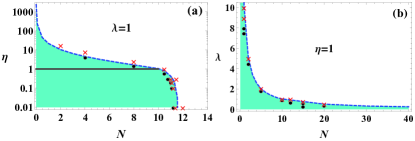
Figure 2: (Color online) 3D stable solitons are predicted by the variational calculation in blue shaded regions of the respective parameter planes. In panel (a), these are SVs (semi-vortices) at $\eta<1$, and MMs (mixed modes) at $\eta>1$, with the boundary between them depicted by the black solid line. In (b), the entire stability area is filled by the solitons of both types, as the SVs and MMs have equal energies at $\eta=1$. The predictions are accurately confirmed by full numerical simulations, as indicated by red crosses and black dots, which indicate, respectively, the absence and presence of stable solitons for respective sets of parameters.

The red squares in Fig. 3(b) represent the variational results for the soliton’s chemical potential, $\mu$, plotted as a function of norm $N$ for $g=\lambda=1$ and $\eta=0.3$. In agreement with the analytical prediction given by Eq. (11), there is no threshold (minimum norm) necessary for the appearance of the solitons, which exist up to a $N=N_{\max}$. Furthermore, the negative slope of the dependence, $d\mu/dN<0$, of the upper branch is an indication of the stability of the soliton families, pursuant to the Vakhitov-Kolokolov (VK) criterion Collapse1 ; Sakaguchi ; VK . The lower branch, which does not satisfy the VK criterion, represents solitons corresponding to the energy maximum on the blue dashed curve in Fig. 1. In the limit of $\mu\to-\infty$, they carry over into the well-known strongly unstable 3D solitons of the GPE Silberberg .

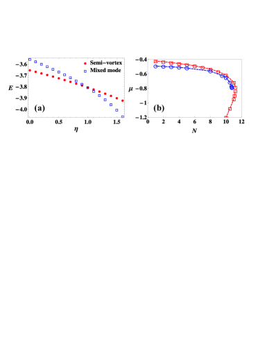
Figure 3: (Color online) (a) Energies of the SVs and MMs, as predicted by the variational approach for $g=\lambda=1$ and $N=8$. The two curves cross at $\eta=1$, where the SV and MM have equal energies. (b) The numerically (blue circles) and variationally (red squares) found chemical potential vs. the norm for the SVs at $g=\lambda=1$ and $\eta=0.3$. The numerical branch extends up to $N=N_{\max}$, in agreement with Eq. (11).

Full numerical calculations — The prediction for the existence of the stable 3D solitons in free space, provided by the analytical approximations, calls for verification by direct simulations of GPE (6). First, we generated stationary states by running the simulations in imaginary time. Typical examples of the so produced SV and MM density profiles are displayed in Fig. 4. Symbols in Fig. 2, which indicate the absence and presence of stable solitons, are in good agreement with the VA.

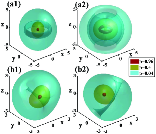
Figure 4: (Color online) Density profiles of 3D solitons for $N=8$ and $g=\lambda=1$. (a) An SV for $\eta=0.3$, whose fundamental and vortical components, $|\psi_{+}|$ and $|\psi_{-}|$, are plotted in (a1) and (a2), respectively. (b) An MM for $\eta=1.5$, with (b1), (b2) displaying $|\psi_{+}|$ and $|\psi_{-}|$, respectively. In each subplot, different colors represent constant-magnitude surfaces, $|\psi_{\pm}|=\left(0.96,0.4,0.04\right)\times|\psi_{\pm}|_{\mathrm{max}}$.

The blue circles in Fig. 3(b) represent the numerically obtained chemical potential, which are in good agreement with the prediction of the VA. The unstable branch from the VA, however, cannot be produced by the imaginary-time integration. We have verified the stability of the solitons belonging to the upper branch in Fig. 3(b) by real-time simulations with random perturbations added to the initial conditions, confirming that the VA accurately predicts the SV and MM stability areas which are displayed in Figs. 2 and 3.

Setting quiescent solitons in motion is another nontrivial issue, as the SOC terms break the Galilean invariance of the system. To construct solitons moving along the $z$-axis with velocity $v_{z}$, so that $\psi_{\pm}=\psi_{\pm}(r,\phi,z-v_{z}t,t)$, we have rewritten the GPE system (6) in the respective moving reference frame. In this form, the velocity term affects the SOC strength along the $z$ axis, breaking the symmetry between the two components of the spinor. As a result, positive (negative) $v_{z}$ tends to increase the population of the spin-down (-up) component. In Fig. 5, we plot the ratio of the spin populations as a function of $v_{z}$. Both VA and numerical results are displayed, showing qualitatively similar results. At $v_{z}<-0.9$ and $v_{z}>+0.4$, the moving semi-vortex practically degenerates into a single-component soliton – the fundamental or vortical one, respectively – thus reducing the setting to that for the single GPE with the cubic self-attraction, where all 3D solitons are strongly unstable. Consequently, the speed of the stably moving solitons cannot be too large.

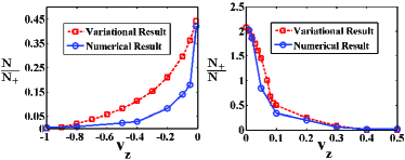
Figure 5: (Color online) The ratio of the spin populations as a function of velocity $v_{z}$ for the moving SV with $N=8$, $g=\lambda=1$, $\eta=0.3$, and $N_{\pm}\equiv\int d^{3}{r}\,|\psi_{\pm}(\mathbf{r})|^{2}$. The red dashed lines with squares are variational results, while the blue solid lines with circles are obtained numerically, using the imaginary-time integration in the moving reference frame.

Finally, to consider collisions between moving solitons, we place two solitons centered at initial positions $(r,z)=(0,\pm z_{0})$, and include a trapping potential, $\Omega^{2}(r^{2}+z^{2})/2$. The solitons then start moving to collide at the trap center, with the trapping frequency $\Omega$ used to control the collision velocity. Figure 6 depicts two collision events for the same initial soliton pair. In panel (a), the slowly moving solitons feature a quasi-elastic collision, while in (b) the collision leads to destruction of faster solitons. This shows the solitons are robust against slow collisions.

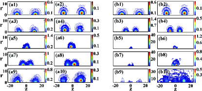
Figure 6: (Color online) Collisions of stable 3D SVs in the harmonic trap for $N=8$, $g=\lambda=1$, and $\eta=0.3$. Panels (a1, a2), (a3, a4), (a5, a6), (a7, a8) and (a9, a10) display density distributions for $\Omega=0.5$ at $t=0$, $1.2$, $3.2$, $4$ and $6$, respectively. Panels (b1, b2), (b3, b4), (b5, b6), (b7, b8) and (b9, b10) display the distributions for $\Omega=1$ at $t=0$, $1$, $1.4$, $2$ and $3$, respectively. In all panels, the left and right subplots display, severally, $|\psi_{+}|$ and $|\psi_{-}|$.

Conclusion — The combination of the analytical and numerical methods reveals that stable free-space 3D solitons can be supported in the binary atomic condensate with attractive interactions and properly engineered SOC, notwithstanding the presence of the supercritical collapse in the same setting. This is the first example of metastable solitons in the 3D homogeneous environment with local cubic self-attraction, which exist in spite of the nonexistence of the GS (ground state) in the system. The SOC plays a crucial role for the stabilization, altering the energy of the self-trapped states so as to create the local energy minimum. This is the fundamental difference from the recently discovered stabilization mechanism in 2D Sakaguchi , which readily creates a missing GS below the critical value of the norm (at $N<N_{\mathrm{cr}}$), where solitons, if any, cannot be destabilized by the critical collapse, as it does not occur at $N<N_{\mathrm{cr}}$, but no solitons could be created at $N\geq N_{\mathrm{cr}}$. In 3D, the existence of the metastable solitons is controlled not by the norm [in an appropriate parameter region, they can be created for any $N$, although the appropriate region becomes very narrow for very large $N$, as seen in Fig. 2(b)], but by the energy, as the above analysis clearly shows.

Although we have adopted the isotropic SOC term in the Hamiltonian, in the form of $\lambda\mathbf{p}\cdot{\boldsymbol{\sigma}}$, the stabilization of the 3D solitons does not critically depend on this form, additional analysis demonstrating that the metastable 3D solitons exist as well if the SOC strength is different along different axes. It may also be interesting to find out if 3D solitons can be stabilized by spatially localized SOC (for 1D solitons, this setting was studied in Ref. localized , but the stability is not an issue in that case). Influence of the Zeeman splitting, which breaks the up-down symmetry of the spinor components, on the stability of the solitons is another relevant problem for further analysis.

On the experimental side, 2D SOC was recently created in an ultracold Fermi gas 2d . Realization of 3D SOC may be expected in the near future, as there is no fundamental obstacle for doing that.

ZWZ acknowledges support from the Strategic Priority Research Program (B) of the CAS, Grant No. XDB01030200 and National Natural Science Foundation of China (Grant No. 11574294,11174270). HP acknowledges support from US NSF and the Welch Foundation (Grant No. C-1669). BAM appreciates a partial support from the Binational (US-Israel) Science Foundation (grant No. 2010239), and hospitality of the Department of Physics and Astronomy at the Rice University.

References

- (1) Y. S. Kivshar and G. P. Agrawal, Optical Solitons: From Fibers to Photonic Crystals (Academic Press, San Diego, 2003); T. Dauxious and M. Peyrard, Physics of Solitons (Cambridge University Press, Cambridge, 2006); J. Yang, Nonlinear Waves in Integrable and Nonintegrable Systems (SIAM, Philadelphia, 2010).
- (2) N. R. Cooper, Phys. Rev. Lett. 82, 1554 (1996).
- (3) E. Babaev, Phys. Rev. Lett. 88, 177002 (2002).
- (4) A. Neubauer, C. Pfleiderer, B. Binz, A. Rosch, R. Ritz, P. G. Niklowitz, and P. Böni, Phys. Rev. Lett. 102, 186602 (2009).
- (5) J. Ruostekoski, and J. R. Anglin, Phys. Rev. Lett. 86, 3934 (2001); T. Kawakami, T. Mizushima, M. Nitta, and K. Machida, ibid. 109, 015301 (2012).
- (6) R. Alkofer, H. Reinhardt, and H. Weigel, Phys. Rep. 265, 139 (1996); M. Bender, P.-H. Heenen, and P.-G. Reinhard, Rev. Mod. Phys. 75, 121 (2003).
- (7) H. Aratyn, L. A. Ferreira, and A. H. Zimerman, Phys. Rev. Lett. 83, 1723 (1999); E. Babaev, L. D. Faddeev, and A. J. Niemi, Phys. Rev. B 65, 100512 (2002); B. Kleihaus, J. Kunz, and Y. Shnir, Phys. Rev. D 68, 101701 (2003); J. Kunz, U. Neemann, and Y. Shnir, Phys. Lett. B 640, 57 (2006); E. Radu, and M. S. Volkov, Phys. Rep. 468, 101 (2008).
- (8) M. I. Weinstein, Commun. Math. Phys. 87, 567 (1983); L. Bergé, Phys. Rep. 303, 259 (1998); G. Fibich, and G. Papanicolaou, SIAM J. Appl. Math. 60, 183 (1999).
- (9) C. Sulem, and P.-L. Sulem, The Nonlinear Schrödinger Equation (Springer, New York, 1999).
- (10) E. A. Kuznetsov, and F. Dias, Phys. Rep. 507, 43 (2011); V. E. Zakharov, and E. A. Kuznetsov, Physics Uspekhi 55, 535 (2012).
- (11) G. A. Swartzlander and C. T. Law, Phys. Rev. Lett. 69, 2503 (1992); Y. S. Kivshar and G. P. Agrawal, Optical Solitons: From Fibers to Photonic Crystals (Academic Press, San Diego, 2003).
- (12) F. Dalfovo, and S. Stringari, Phys. Rev. A 53, 2477 (1996); R. J. Dodd, J. Res. Natl. Inst. Stand. Technol. 101, 545 (1996); T. J. Alexander, and L. Bergé, Phys. Rev. E 65, 026611 (2002); L. D. Carr, and C. W. Clark, Phys. Rev. Lett. 97, 010403 (2006).
- (13) H. Morise, and M. Wadati, J. Phys. Soc. Jpn. 70, 3529 (2001).
- (14) B. B. Baizakov, B. A. Malomed, and M. Salerno, Europhys. Lett. 63, 642 (2003); J. Yang and Z. H. Musslimani, Opt. Lett. 28, 2094 (2003).
- (15) B. B. Baizakov, B. A. Malomed, and M. Salerno, Phys. Rev. A 70, 053613 (2004); D. Mihalache, D. Mazilu, F. Lederer, Y. V. Kartashov, L.-C. Crasovan, and L. Torner, Phys. Rev. E 70, 055603(R) (2004).
- (16) D. Mihalache, D. Mazilu, F. Lederer, B. A. Malomed, L.-C. Crasovan, Y. V. Kartashov and L. Torner, Phys. Rev. A 89, 021601(R) (2005).
- (17) D. Mihalache, D. Mazilu, L.-C. Crasovan, I. Towers, A. V. Buryak, B. A. Malomed, L. Torner, J. P. Torres, and F. Lederer, Phys. Rev. Lett. 88, 073902 (2002).
- (18) Y. V. Kartashov, B. A. Malomed, and L. Torner, Rev. Mod. Phys. 83, 247 (2011).
- (19) E. L. Falcão-Filho, C. B. de Araújo, G. Boudebs, H. Leblond, and V. Skarka, Phys. Rev. Lett. 110, 013901 (2013).
- (20) O. V. Borovkova, Y. V. Kartashov, L. Torner, and B. A. Malomed, Phys. Rev. E 84, 035602 (R) (2011); R. Driben, Y. V. Kartashov, B. A. Malomed, T. Meier, and L. Torner, Phys. Rev. Lett. 112, 020404 (2014); Y. V. Kartashov, B. A. Malomed, Y. Shnir, and L. Torner, ibid. 113, 264101 (2014); R. Driben, Y. Kartashov, B. A. Malomed, T. Meier, and L. Torner, New J. Phys. 16, 063035 (2014); R. Driben, N. Dror, B. Malomed, and T. Meier, ibid. 17, 083043 (2015).
- (21) W. Królikowski, O. Bang, N. I. Nikolov, D. Neshev, J. Wyller, J. J. Rasmussen, and D. Edmundson, J. Opt. B: Quantum Semiclass. Opt. 6, S288 (2004); F. Maucher, N. Henkel, M. Saffman, W. Królikowski, S. Skupin, and T. Pohl, Phys. Rev. Lett. 106, 170401 (2011).
- (22) I. Tikhonenkov, B. A. Malomed, and A. Vardi, Phys. Rev. Lett. 100, 090406 (2008).
- (23) We are only concerned with bright solitons supported by attractive nonlinearity. Dark solitons may exist in systems with repulsive nonlinearity, but their physical realization always requires some confinement potential and hence can never exist in free space.
- (24) H. Sakaguchi, B. Li and B. A. Malomed, Phys. Rev. E 89, 032920 (2014); H. Sakaguchi and B. A. Malomed, ibid. 90, 062922 (2014).
- (25) Y.-J. Lin, K. Jiménez-García and I. B. Spielman, Nature, 471, 83 (2011).
- (26) V. Achilleos, D. J. Frantzeskakis, P. G. Kevrekidis, and D. E. Pelinovsky, Phys. Rev. Lett. 110, 264101 (2013); Y. V. Kartashov, V. V. Konotop, and F. Kh. Abdullaev, ibid. 111, 060402 (2013); Y. Xu, Y. Zhang, and B. Wu, Phys. Rev. A 87, 013614 (2013); L. Salasnich and B. A. Malomed, ibid. 87, 063625 (2013); P. Beličev, G. Gligorić, J. Petrović, A. Maluckov, L. Hadžievski, and B. Malomed, J. Phys. B At. Mol. Opt. Phys. 48, 065301 (2015).
- (27) R. Y. Chiao, E. Garmire and C. H. Townes, Phys. Rev. Lett. 13, 479 (1964).
- (28) Y. V. Kartashov, B. A. Malomed, V. V. Konotop, V. E. Lobanov, and L. Torner, Opt. Lett. 40, 1045 (2015).
- (29) K. S. Chiang, Opt. Lett. 20, 997 (1995); J. Opt. Soc. Am. B 14, 1437 (1997).
- (30) J. Dalibard, F. Gerbier, G. Juzeliūnas, and P. Öhberg, Rev. Mod. Phys. 83, 1523 (2011); N. Goldman, G. Juzeliūnas, P. Öhberg, and I. B. Spielman, Rep. Prog. Phys. 77, 126401 (2014); H. Zhai, ibid. 78, 026001 (2015).
- (31) B. M. Anderson, G. Juzeliūnas, V. M. Galitski, and I. B. Spielman, Phys. Rev. Lett. 108, 235301 (2012).
- (32) While Eqs. (7) and (8) are generic exact ansätze for the semi-vortex solution of the GPE (6), Eq. (9) is exact solely for .
- (33) M. Vakhitov, and A. Kolokolov, Radiophys. Quantum Electron. 16, 783 (1973).
- (34) Y. Silberberg, Opt. Lett. 15, 1282 (1990).
- (35) Y. V. Kartashov, V. V. Konotop, and D. A. Zezyulin, Phys. Rev. A 90, 063621 (2014).
- (36) L. Huang, Z. Meng, P. Wang, P. Peng, S.-L. Zhang, L. Chen, D. Li, Q. Zhou, and J. Zhang, arXiv:1506.02861.