Robust Gaussian Filtering using a Pseudo Measurement
Abstract
Many sensors, such as range, sonar, radar, GPS and visual devices, produce measurements which are contaminated by outliers. This problem can be addressed by using fat-tailed sensor models, which account for the possibility of outliers. Unfortunately, all estimation algorithms belonging to the family of Gaussian filters (such as the widely-used extended Kalman filter and unscented Kalman filter) are inherently incompatible with such fat-tailed sensor models. The contribution of this paper is to show that any Gaussian filter can be made compatible with fat-tailed sensor models by applying one simple change: Instead of filtering with the physical measurement, we propose to filter with a pseudo measurement obtained by applying a feature function to the physical measurement. We derive such a feature function which is optimal under some conditions. Simulation results show that the proposed method can effectively handle measurement outliers and allows for robust filtering in both linear and nonlinear systems.
100mm(.-10.5cm)
2016 American Control Conference
July 6-8, 2016, Boston, MA, USA
I Introduction
Robust and accurate state estimation is essential to safely control any dynamical system. However, many sensors, such as range, sonar, radar, GPS and visual devices, provide measurements populated with outliers. Therefore, the estimation algorithm must not be unduly affected by such outliers.
In this paper we argue that problems with outliers are a direct consequence of unrealistic, thin-tailed sensor models. Unfortunately, many widely-used estimation algorithms are inherently incompatible with more realistic, fat-tailed sensor models. This holds true for the extended Kalman filter (EKF) [1], the unscented Kalman filter (UKF) [2], and any other member of the family of Gaussian filters (GF) [3], as we will show in Section IV-A.
The contribution of this paper is to show that any member of the family of GFs can be made compatible with fat-tailed sensor models by applying one simple change: Instead of filtering with the physical measurement, we filter with a pseudo measurement. This pseudo measurement is obtained by applying a time-varying feature function to the physical measurement. We derive a feature function which is optimal under some conditions. In simulation experiments, we demonstrate the robustness and accuracy of the proposed method for linear as well as nonlinear systems.
Numerous robustification methods have been proposed for individual members of the family of GFs, often involving significant algorithmic changes. In contrast, the proposed method can be applied to any GF with only minor changes in the implementation. Any existing GF implementation can be robustified by merely replacing the sensor model with a pseudo sensor model, and the physical measurement with a pseudo measurement.
II Related Work
Ad-hoc procedures for reducing the influence of outliers have been employed by engineers for a long time. One such heuristic is to simply discard all measurements which are too far away from the expected measurement. This approach lacks a firm theoretical basis and there is no rigorous way of choosing the thresholds. Furthermore, the information contained in measurements outside of the thresholds is discarded completely, which can lead to decreased efficiency [4]. For these reasons, significant research effort has been devoted to robustifying GFs in a principled manner. In the following we distinguish two main currents on robust filtering, the first is based on robust statistics in the sense of [5] and the second is based on fat-tailed sensor models.
II-A Robust Statistics
In the framework of robust statistics in the spirit of [5], the objective is to find an estimator with a small variance when the Gaussian noise is contaminated with noise from a broad class of distributions. The resulting estimators are intermediary between the sample mean and the sample median. For instance, Masreliez and Martin [6] propose such an estimator for linear systems. This approach is extended by Schick and Mitter [4]. inline,color=red!40]Cristina: remove: However, these approaches are restricted to linear systems.
II-B Fat-tailed Sensor Models
Since fat-tailed sensor models are by definition non-Gaussian, finding the posterior estimate is not trivial. In particular, a lot of effort has been devoted to finding filtering recursions for models with Student -distributed noise.
Roth et al. [7] show that for linear systems where the noise and the state are jointly -distributed, an exact filter can be found. The authors mention that these noise conditions are rarely met in practice, and propose an approximation for state-independent -distributed noise. A different approximation scheme for linear systems with -distributed noise is proposed in Meinhold and Singpurwalla [8].
II-C Extensions to Nonlinear Systems
All methods mentioned above assume a linear sensor model. It is possible to apply them to nonlinear systems by linearizing the sensor model at each time step, as is done in the EKF. However, the EKF has been shown to yield poor performance for many nonlinear systems [13, 2, 14].
Application of these robustification methods to other members of the family of GFs, such as the UKF or the divided difference filter (DDF) [15], is not straightforward.
One way of doing so is proposed by Karlgaard and Schaub [16], who use a robust Huber estimator [5] in a DDF. Similarly, Piche et al. [17] propose a method of extending the mentioned linear Student -based filtering methods to nonlinear GFs. However, both of these methods rely on an iterative optimization at each time step, which is computationally expensive. In contrast, the robustification proposed in this paper allows to robustify any of the numerous GF algorithms with just minor changes in the implementation.
III Filtering
A discrete-time state-space model can be defined by two probability distributions: a transition model , which describes the evolution of the state in time, and a sensor model , which describes how the measurement is generated given the state . Alternatively, these two models can also be written in functional form
| (1) | ||||
| (2) |
with and being normally distributed noise variables. Note that any (even non-Gaussian) model can be specified in this way, since and can be mapped onto any desired distribution inside the nonlinear functions and .
III-A Exact Filtering
Filtering is concerned with estimating the current state given all past measurements . The posterior distribution of the current state can be computed recursively from the distribution of the previous state . This recursion can be written in two steps: a prediction step111We use the notation as an abbreviation for .
| (3) |
and an update step
| (4) |
These equations can generally not be solved in closed form [18]. The most notable exception is the Kalman filter (KF) [19], which provides the exact solution for linear Gaussian systems. Significant research effort has been invested into generalizing the KF to nonlinear dynamical systems.
III-B Gaussian Filtering
The KF and its generalizations to nonlinear systems (e.g. the EKF and the UKF) are members of the family of GFs [3, 20, 14, 21]. GFs approximate both the predicted belief (3), as well as the posterior belief (4) with Gaussian distributions.
In the prediction step (3), the exact distribution is approximated by a Gaussian222 denotes the Gaussian with mean and covariance .
| (5) |
The prediction step is not affected by the type of sensor model used and will therefore not be discussed here, see for instance [3, 20, 14, 21] for more details.
We will only consider the update step (4) in the remainder of the paper. For ease of notation, we will not write the dependence on past measurements explicitly anymore. The remaining variables all have time index , which can therefore be dropped. The predicted belief can now simply be written as , and the posterior belief as , etc.
As shown in [20], the GF can be understood as finding an approximate Gaussian posterior by minimizing the Kullback-Leibler divergence [22] to the exact joint distribution
| (6) |
The form of is restricted to be Gaussian in
| (7) |
with the mean being an affine function of
| (8) |
This minimization is performed at each update step and yields the optimal parameters of the approximation (7)
| (9) | ||||
| (10) |
See [20] for a detailed derivation of this result. The parameters and are given by the belief (5) computed in the prediction step. The remaining parameters are defined as
| (11) | ||||
| (12) | ||||
| (13) |
For a linear system, this solution corresponds to the KF equations [20].
Numeric Integration Methods
For most nonlinear systems, the integrals (11), (12) and (13) cannot be computed in closed form and have to be approximated. In the EKF, this is done by linearization at the current mean estimate of the state . This approximation does not take the uncertainty in the estimate into account, which can lead to large errors and sometimes even divergence of the filter [13, 14].
Therefore, approximations based on numeric integration methods are preferable in most cases. Deterministic Gaussian integration schemes have been investigated thoroughly, and the resulting filters are collected under the term Sigma Point Kalman Filters (SPKF) [13]. Well known members of this family are the UKF [2], the DDF [15] and the cubature Kalman filter (CKF) [23]. Alternatively, numeric integration can also be performed using Monte Carlo methods. The method presented in this paper applies to any GF, regardless of which particular integration method is used.
IV A Case for Fat Tails
Measurement acquisition is typically modeled by a Gaussian or some other thin-tailed sensor model. This assumption is usually made for analytical convenience, not because it is an accurate representation of the belief of the engineer. If an engineer were to believe that measurements are in fact generated by a Gaussian distribution, then she would have to accept a betting ratio of to that no measurement further than standard deviations from the state will occur.333According to De Finetti’s definition of probability [24]. Few engineers would be interested in such a bet, since one can usually not exclude the possibility of acquiring a large measurement due to unexpected physical effects in the measurement process.
The mismatch between the actual belief and the Gaussian model can lead to counter-intuitive behavior of the inference algorithm. More concretely, the posterior mean is an affine function of the measurement. This implies that the shift in the mean produced by a single measurement is not bounded.
This problematic behavior disappears when using a more realistic, fat-tailed model instead of the Gaussian model [8]. There are several definitions of fat-tails which are commonly used [25]. Here, we simply mean any distribution which decays slower than the Gaussian. Which particular tail model is used depends on the application.
IV-A The Gaussian Filter using Fat Tails
The GF approximates all beliefs with Gaussians, but the sensor model can have any form. In principle, nothing prevents us from using the GF with a fat-tailed sensor model. Unfortunately, the GF is not able to do proper inference using such a model. The sensor model enters the GF equations only through (11), (12) and (13). To make this dependency explicit, we substitute in (11) and (12), and in (13), and integrate in
| (14) | ||||
| (15) | ||||
| (16) |
What is important to note here is that these equations only depend on the sensor model through the conditional mean and the conditional covariance
| (17) | ||||
| (18) |
Since fat-tailed sensor models typically have very large or even infinite covariances, the GF will behave as if the measurements were extremely noisy. It achieves robustness by simply discarding all measurements, which is obviously not the behavior we were hoping for.
IV-B Simulation Example

To illustrate this problematic behavior, we apply the GF to the following dynamical system:
Example IV.1
System specification444 denotes the Cauchy distribution with location and scale .
| (19) | ||||
| (20) | ||||
| (21) |
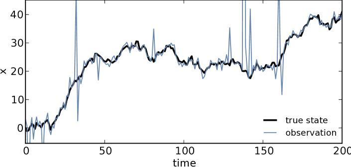
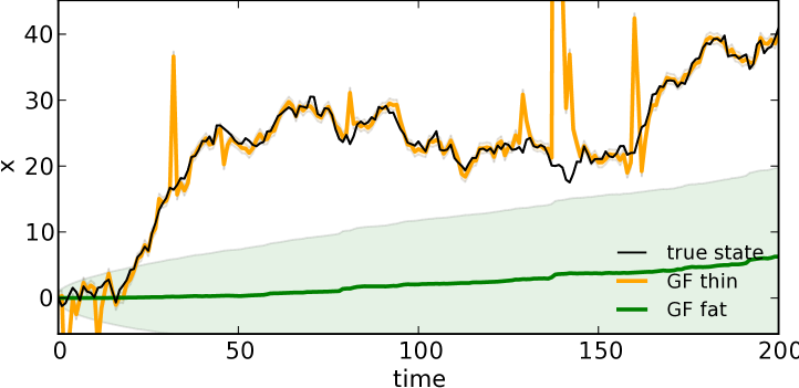
The measurements are contaminated with Cauchy-distributed noise, which leads to occasional outliers, as shown in Figure 1. We apply two GFs to this problem. The first uses a sensor model which does not take into account the fat-tailed Cauchy noise, it only models the Gaussian noise, i.e. the left term in (20). The second GF uses a sensor model which is identical to the true sensor (20). We will refer to the first filter as the thin-tailed GF, and to the second filter as the fat-tailed GF.
In Figure 2(a), we show the exact density after the first filtering step. The approximations obtained by the thin-tailed GF (yellow) and the fat-tailed GF (green) are overlaid. It can be seen that the approximation to the exact posterior is very poor in both cases. The mean of the exact density is approximately linear in for small . For measurements larger than about , the posterior mean reverts back to the prior mean and does not depend on anymore.
This behavior cannot be captured by an approximation of the form of (8), since it only allows for linear dependences in . The approximation by the thin-tailed GF fits the exact posterior well for small , but instead of flattening out it keeps growing linearly for large . Hence, it is not robust to outliers. The approximation by the fat-tailed GF correctly captures the behavior of the exact posterior for large , i.e. it is independent of . However, this implies that all measurements, not just outliers, are ignored, as expected from the analysis in Section IV-A. For both filters, the poor fit translates to poor filtering performance, as shown in Figure 2(b).
V A Measurement Feature for Robustification
To enable the GF to work with fat-tailed sensor models, we hence have to change the form of the approximate belief (7). In [20] it is shown that more flexible approximations can be obtained by allowing for nonlinear features in . The mean function (8) then becomes
| (22) |
The resulting filter is equivalent to the standard GF using a virtual
measurement which is obtained by applying a nonlinear feature function
to the physical measurement.
inline,color=red!40]Cristina: removed:
. This feature function can be time-varying, and may depend on
the current belief
In the following, we find a feature which enables the GF to work with fat-tailed sensor models. Instead of hand-designing such a feature, we attempt to find a feature which is optimal in the sense that it minimizes the KL divergence between the exact and the approximate distribution (6).
For this purpose, we first find the optimal, non-parametric mean function with respect to (6). Knowing that the mean is an affine function (22) of the feature , we can then deduce the optimal feature function .
V-A The Optimal Mean Function
In order to find the function which minimizes (6), we rewrite the objective (6)
| (23) | ||||
| (24) |
where we have collected the terms independent of in . Since there is no constraint on , (24) can be optimized for each independently. This means that the integral can be dropped, and we can simply minimize the integrand with respect to . It is a standard result from variational inference that the optimal parameters of a Gaussian approximation are obtained by moment matching [26]. That is, the optimal mean function of the approximation is simply equal to the exact posterior mean
| (25) |
Therefore, the feature vector would ideally be chosen such that can be expressed through a linear combination of features. Unfortunately, cannot be found in closed form in most cases.
The standard GF represents the mean of the posterior as an affine function of . This form is optimal for linear Gaussian systems, and it serves as a good approximation for many nonlinear thin-tailed systems. Similarly, the idea here is to find the optimal feature for a linear Gaussian system with an additive fat tail. This feature can be expected to provide a good approximation for nonlinear fat-tailed systems.
V-B The Optimal Feature for a Linear, Fat-Tailed Sensor
Suppose that we have a linear Gaussian sensor model
| (26) |
which we refer to as the body. We would like to add a fat tail to make the filter robust to outliers. The combined sensor model with tail weight is then
| (27) |
V-B1 Assumptions on the Form of the Tail
The precise shape of the tail is application specific and does not matter for the ideas in this paper. However, the subsequent derivation relies on the assumption that the tail is almost constant in on the length scale of the standard deviation of the belief . This allows us to treat like a Dirac function with respect to . More concretely, we will assume that the approximation
| (28) |
is accurate for any affine function .
This is a reasonable assumption, since the tail accounts for unexpected effects in the measurement process, which by definition bear little or no relation to the state . For instance, Thrun et al. [27] suggest to use a tail which is independent of the state and uniform in , to account for outliers in range sensors. For such uniform tails, (28) is exact. For state-dependent tails, we expect this approximation to be accurate enough to provide insights into the required form of the feature.
V-B2 The Conditional Mean
We will now find the posterior mean for this measurement model, which will then allow us to find the optimal feature. The posterior mean can be obtained from the predicted belief and the sensor model using Bayes’ rule
| (29) |
Inserting (27) we obtain
| (30) |
Both the predicted belief and the body of the sensor model are Gaussian. Therefore, the integrals in the first term of the numerator and the first term in the denominator can be solved analytically using standard Gaussian marginalization and conditioning. The integrals in the second terms of the numerator and the denominator can be approximated according to (28), and we obtain
| (31) | ||||
| (32) |
where we have defined
| (33) | ||||
| (34) |
The expectations in (32)
| (35) |
only involve the body, and not the tail distribution. Hence, we avoid the problems related to the potentially huge or even infinite covariance of the tail discussed in Section IV-A.
In Figure 3, we plot the optimal mean function (32) for dynamical system in Example IV.1 (at time ).
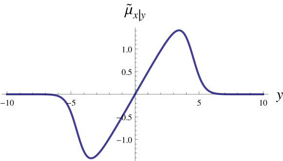
For close to the expected measurement , the conditional mean (32) is approximately linear in . If a measurement of large magnitude is obtained, then the tail becomes predominant, and the posterior mean reverts to the prior mean .
V-B3 The Optimal Feature
To identify the feature required to express the optimal mean , we compare (32) to (22). All the constant terms can be collected in and all the terms which depend on are part of the feature555 The factors and in the numerator could equally well have been collected in instead of the feature, since they are constant. However, we prefer to maintain these terms in the feature since they provide appropriate scaling.
| (36) |
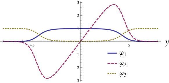
All of the feature components are asymptotically constant in , which means that the estimate remains bounded for arbitrarily large measurements. The three components have intuitive interpretations. The first two components are approximately constant and linear in respectively, for measurements close to the expected value. Hence, they allow the filter to express an affine dependence on which will vanish for very large measurements. The third component is small for close to the expected value, and grows up to some constant for which are large. It hence allows the mean estimate to revert to a constant value for large measurements.
VI The Robust Gaussian Filter
In the previous section, we found the approximately optimal measurement feature for a linear Gaussian sensor model with additive fat tails. The GF can hence be enabled to work with fat-tailed sensor models by filtering in feature space. This robustification can be applied to any member of the family of GFs, be it the EKF or an SPKF. We will refer to the filter obtained by using the feature (36) as the robust Gaussian filter (RGF).
For nonlinear, fat-tailed models, the RGF will not be optimal, but it provides a good approximation in the same way the standard GF provides a good approximation to nonlinear, thin-tailed sensor models. If the RGF is applied to a sensor model without a fat tail, it will coincide with the standard GF, since the feature reduces to a linear function (37). Hence, the RGF extends the GF. It broadens its domain of applicability to fat-tailed sensor models.
Algorithm
For clarity, we describe the RGF algorithm here step by step. Since this involves variables of several time steps, we will reintroduce the time indices which we dropped earlier.
The standard GF is described in Algorithm 1.
The input to the algorithm are the previous belief, the new measurement , the transition model (1) and the sensor model (2). The GF simply predicts, then updates, and finally returns the new estimate. The concrete implementation of the predict and the update functions depends on whether we are using an EKF, a UKF, a DDF or some other GF.
The RGF is described in Algorithm 2. It requires the same inputs as the GF, and additionally the separate components of the sensor model: body, tail, and tail weight. In particular, the functional form of the body is used in Step 2, while the feature computation in Step 3 requires the tail weight and the evaluation of the tail’s distribution .
The RGF delegates all the main computations to the basic GF through the predict and the update functions. The overhead in the implementation and in the computational cost is minor. Hence, the proposed method makes it straightforward to robustify any existing GF algorithm.
VII Simulation Experiments
In this section, we evaluate the RGF through simulations. First, we show that the optimal feature enables a good fit of the approximate belief to the exact posterior in the linear system used in previous sections. Secondly, we evaluate the sensitivity of the RGF to the choice of tail parameters (Section VII-B). Finally, we show that the proposed feature (36), which we designed for a linear system, also allows for robustification in nonlinear systems (Section VII-C).
We implemented Algorithm 2 using Monte Carlo as method for the numeric integration required by the predict and the update functions666Code is available at https://git-amd.tuebingen.mpg.de/amd-clmc/python_gaussian_filtering.
VII-A Application to a Linear Filtering Problem
We revisit the simulation in Example IV.1 applying this time the RGF, using the true transition and sensor models.
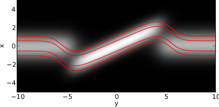
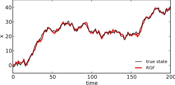
Comparing Figure 2(a) to Figure 5(a), it is clear that the feature (36) allows for a much better fit of the approximation to the true density. As expected, this improved fit translates to a better filtering performance (Figure 5(b)). As desired, the proposed method is sensitive to measurements close to the expected values, but does not react to extreme values.
VII-B Robustness to Tail Parameters
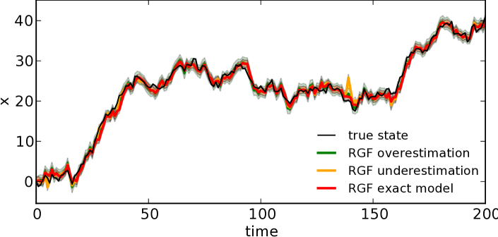
To show that the RGF is not sensitive to the specific choice of the tail parameters, we simulate the same system as above, and run several RGFs with different tail parameters. First, we apply a RGF using a sensor model matching the true sensor, i.e. with tail parameters , . Then, we apply two RGFs which use incorrect tail parameters. In one case we make both the weight and scale of the tail much lower than in the true distribution: , (underestimation of the true tail). In the other case we make them much higher: , (overestimation). Figure 6 shows almost no degradation in the performance. The key aspect enabling good filtering performance is that the sensor model has a tail which decays slower than the Gaussian distribution, even when the shape of the true tail is not precisely known.
| value | units | value | units | ||
|---|---|---|---|---|---|
| s | km | ||||
| km/ | km | ||||
| /km | mrad | ||||
| km | mrad | ||||
| km |
VII-C Application to a Nonlinear Filtering Problem
As an example of nonlinear filtering, we consider the problem of using measurements from a radar ground station to track the position of a vehicle that enters the atmosphere at high altitude and speed. inline,color=red!40]Cristina: removed: The main forces acting on the vehicle are the aerodynamic drag and gravity. The measurements provided by the radar are range and bearing angle to the target vehicle. This type of problem has been used before to compare the capability of filters to deal with strong nonlinearities, e.g. [28, 16].
The noise in radar systems is typically referred to as glint noise in the literature, and is known to be contaminated with outliers [29, 30, 16, 31, 32]. It has been modeled in different ways, e.g. using a Student distribution, or as a mixture of two zero-mean Gaussian distributions (one with high weight and low variance and another with low weight and high variance), see [31] and references therein. In this section, we simulate the same system as in [28], but replace their Gaussian measurement noise with a mixture of two Gaussians as in [16, 31].
State Transition Process
The state consists of the position of the vehicle , its velocity (, ), and an unknown aerodynamics parameter , which has to be estimated. The state dynamics are
| (38) | ||||
| (39) | ||||
| (40) | ||||
| (41) | ||||
| (42) |
where and follow a standard normal distribution, and is the discretization time step. The drag and gravity coefficients, and , depend on the distance of the object to the centre of the Earth , its speed , and its unknown ballistic coefficient . Other quantities such as the nominal ballistic coefficient and the mass and and radius of the Earth are constant, see Table I.
Sensor Model
Filter Specification
We compare an RGF with two GFs. The three filters use transition models that coincide with the real process (38)–(42).
In problems of this type, the contaminating noise is often not precisely known. Therefore, we make our RGF assume a measurement model as in Example IV.1
| (46) |
which makes use of some knowledge of the nominal noise , while the shape of the tail and the mixing weight take default values. Similarly, the first GF only knows about
| (47) |
As discussed in Section IV-A, the GF is not able to produce accurate estimates in systems with large variance even if the true measurement process (45) is known. To show this empirically, we apply a second GF which uses the true covariance of the sensor (45)
| (48) |
We simulate the system during 100 s, using the integration time step for the predictions and taking radar measurements at 1 Hz. As in [28], the initial state of the system is , and the initial belief for all filters is centered at . Note the mismatch between the true ballistic coefficient and the initial belief, i.e. the nominal .
Results
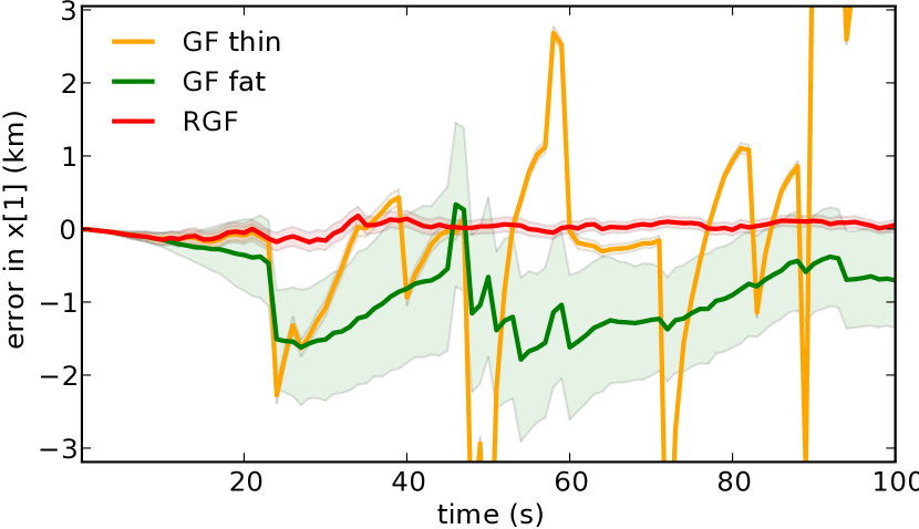
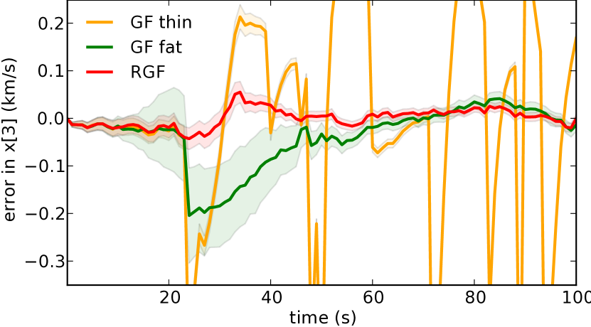
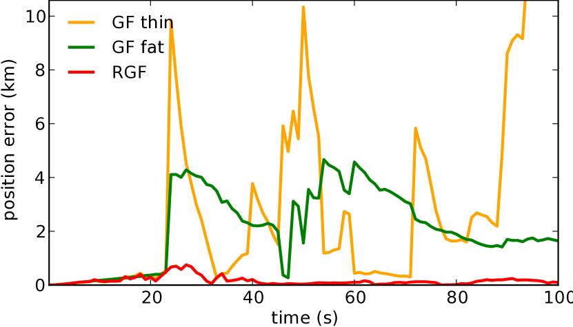
Figures 7(a) and 7(b) respectively show the error in the estimate of and the corresponding velocity . We do not include the error in the position and velocity along the other dimension, since they are qualitatively similar. We can see that the GF using the nominal variance (yellow) reacts strongly to outliers. The GF using the true variance (green) of the sensor does not react as strongly. However, due to the large variance, it tracks the true state poorly. In contrast, the RGF (red) is robust to outliers and at the same time tracks the true state well. This translates to a low 2D location error as shown in Figure 7(c). These results indicate that the optimal feature for linear systems allows to robustify nonlinear systems too.
VIII Conclusion
In the standard GF algorithm, the mean estimate is an affine function of the measurement. We showed that for fat-tailed sensor models this provides a very poor approximation to the exact posterior mean.
A recent result [20] showed that filtering in measurement feature space can allow for more accurate approximations of the exact posterior. Here, we have found the feature that is optimal for fat-tailed sensor models under certain conditions.
We have shown both theoretically and in simulation that applying the standard GF in this feature space enables it to work well with fat-tailed sensor models. The proposed RGF is hence robust to outliers while maintaining the computational efficiency of the standard GF. Any member of the family of GFs, such as the EKF or the UKF, can thus be robustified by the proposed method without changing any of the main computations.
We have applied this algorithm to the problem of 3D object tracking using an Xtion range sensor [33]. The main source of outliers in this application are occlusions of the tracked object. While the standard GF immediately loses track of the object when occlusions occur, the RGF works well even under heavy occlusion.
References
- Sorenson [1960] H. W. Sorenson. Kalman Filtering: Theory and Application. IEEE Press selected reprint series. IEEE Press, 1960.
- Julier and Uhlmann [1997] S. J. Julier and J. K. Uhlmann. A new extension of the Kalman filter to nonlinear systems. In Proceedings of AeroSense: The 11th Int. Symp. on Aerospace/Defense Sensing, Simulations and Controls, pages 182–193, 1997.
- Särkkä [2013] S. Särkkä. Bayesian filtering and smoothing. Cambridge University Press, New York, NY, USA, 2013.
- Schick and Mitter [1994] I. C. Schick and S. K. Mitter. Robust recursive estimation in the presence of heavy-tailed observation noise. The Annals of Statistics, 1994.
- Huber [1964] P. J. Huber. Robust estimation of a location parameter. Annals of Mathematical Statistics, 1964.
- Masreliez and Martin [1977] C. Masreliez and R. Martin. Robust Bayesian estimation for the linear model and robustifying the Kalman filter. IEEE Transactions on Automatic Control, 1977.
- Roth et al. [2013] M. Roth, E. Ozkan, and F. Gustafsson. A Student’s t filter for heavy tailed process and measurement noise. In IEEE International Conference on Acoustics, Speech and Signal Processing (ICASSP), 2013.
- Meinhold and Singpurwalla [1989] R. J. Meinhold and N. D. Singpurwalla. Robustification of Kalman filter models. Journal of the American Statistical Association, 1989.
- Ting et al. [2007] J.-A. Ting, E. Theodorou, and S. Schaal. A Kalman filter for robust outlier detection. In IEEE/RSJ International Conference on Intelligent Robots and Systems (IROS), 2007.
- Särkkä and Nummenmaa [2009] S. Särkkä and A. Nummenmaa. Recursive noise adaptive Kalman filtering by variational Bayesian approximations. IEEE Transactions on Automatic Control, 2009.
- Agamennoni et al. [2011] G Agamennoni, J. I. Nieto, and E. M. Nebot. An outlier-robust kalman filter. In Robotics and Automation (ICRA), 2011 IEEE International Conference on, 2011.
- Agamennoni et al. [2012] G Agamennoni, J. I. Nieto, and E. M. Nebot. Approximate inference in state-space models with heavy-tailed noise. IEEE Transactions on Signal Processing, 2012.
- van der Merwe and Wan [2003] R. van der Merwe and E. Wan. Sigma-Point Kalman Filters for probabilistic inference in dynamic state-space models. In In Proceedings of the Workshop on Advances in Machine Learning, 2003.
- Ito and Xiong [2000] K. Ito and Kaiqi Xiong. Gaussian filters for nonlinear filtering problems. IEEE Transactions on Automatic Control, 45(5):910–927, May 2000.
- NøRgaard et al. [2000] Magnus NøRgaard, Niels K. Poulsen, and Ole Ravn. New developments in state estimation for nonlinear systems. Automatica, 36(11):1627–1638, November 2000. ISSN 0005-1098.
- Karlgaard and Schaub [2006] C. D. Karlgaard and H. Schaub. Comparison of several nonlinear filters for a benchmark tracking problem. In AIAA Guidance, Navigation, and Control Conference and Exhibit, Keystone, CO, USA, august 2006.
- Piche et al. [2012] R. Piche, S. Särkkä, and J. Hartikainen. Recursive outlier-robust filtering and smoothing for nonlinear systems using the multivariate student-t distribution. In IEEE International Workshop on Machine Learning for Signal Processing (MLSP), 2012.
- Kushner [1967] H. J. Kushner. Approximations to optimal nonlinear filters. IEEE Transactions on Automatic Control, 12(5):546–556, 1967.
- Kalman [1960] R. E. Kalman. A New Approach to Linear Filtering and Prediction Problems. Transactions of the ASME - Journal of Basic Engineering, (82 (Series D)):35–45, 1960.
- Wüthrich et al. [2015] M. Wüthrich, S. Trimpe, D. Kappler, and S. Schaal. A New Perspective and Extension of the Gaussian Filter. In Robotics: Science and Systems (R:SS), 2015.
- Wu et al. [2006] Y. Wu, D. Hu, M. Wu, and X. Hu. A numerical-integration perspective on Gaussian filters. IEEE Transactions on Signal Processing, 54(8):2910–2921, 2006.
- MacKay [2003] David J. MacKay. Information Theory, Inference and Learning Algorithms. Cambridge University Press, 2003.
- Arasaratnam and Haykin [2009] I. Arasaratnam and S. Haykin. Cubature Kalman filters. Automatic Control, IEEE Transactions on, 2009.
- de Finetti [1937] B. de Finetti. La prévision : ses lois logiques, ses sources subjectives. Annales de l’institut Henri Poincaré, 1937.
- Cooke et al. [2011] R. Cooke, D. Nieboer, and J. Misiewicz. Fat-tailed distributions: Data, diagnostics, and dependence. Technical report, 2011.
- Barber [2012] D. Barber. Bayesian Reasoning and Machine Learning. Cambridge University Press, New York, NY, USA, 2012.
- Thrun et al. [2001] S. Thrun, D. Fox, W. Burgard, and F. Dellaert. Robust Monte Carlo localization for mobile robots. Artificial Intelligence, 2001.
- Julier and Uhlmann [2004] S. J. Julier and J. K. Uhlmann. Unscented filtering and nonlinear estimation. Proceedings of the IEEE, 2004.
- Hewer et al. [1987] G. A. Hewer, R. D. Martin, and J. Zeh. Robust preprocessing for Kalman filtering of glint noise. IEEE Transactions on Aerospace and Electronic Systems, 1987.
- Wu and Cheng [1994] W.-R. Wu and P.-P. Cheng. A nonlinear IMM algorithm for maneuvering target tracking. IEEE Transactions on Aerospace and Electronic Systems, 1994.
- Bilik and Tabrikian [2006] I. Bilik and J. Tabrikian. Target tracking in glint noise environment using nonlinear non-Gaussian Kalman filter. In IEEE Conference on Radar, 2006.
- [32] H. Du, W. Wang, and L. Bai. Observation noise modeling based particle filter: An efficient algorithm for target tracking in glint noise environment. Neurocomputing.
- Issac et al. [2016] J. Issac, M. Wüthrich, C. Garcia Cifuentes, J. Bohg, S. Trimpe, and S. Schaal. Depth-Based Object Tracking Using a Robust Gaussian Filter. In Robotics and Automation (ICRA), IEEE International Conference on, 2016. URL http://arxiv.org/abs/1602.06157.