Conjugate gradient acceleration of iteratively re-weighted least squares methods

Abstract

Iteratively Re-weighted Least Squares (IRLS) is a method for solving minimization problems involving non-quadratic cost functions, perhaps non-convex and non-smooth, which however can be described as the infimum over a family of quadratic functions. This transformation suggests an algorithmic scheme that solves a sequence of quadratic problems to be tackled efficiently by tools of numerical linear algebra. Its general scope and its usually simple implementation, transforming the initial non-convex and non-smooth minimization problem into a more familiar and easily solvable quadratic optimization problem, make it a versatile algorithm. However, despite its simplicity, versatility, and elegant analysis, the complexity of IRLS strongly depends on the way the solution of the successive quadratic optimizations is addressed. For the important special case of compressed sensing and sparse recovery problems in signal processing, we investigate theoretically and numerically how accurately one needs to solve the quadratic problems by means of the conjugate gradient (CG) method in each iteration in order to guarantee convergence. The use of the CG method may significantly speed-up the numerical solution of the quadratic subproblems, in particular, when fast matrix-vector multiplication (exploiting for instance the FFT) is available for the matrix involved. In addition, we study convergence rates. Our modified IRLS method outperforms state of the art first order methods such as Iterative Hard Thresholding (IHT) or Fast Iterative Soft-Thresholding Algorithm (FISTA) in many situations, especially in large dimensions. Moreover, IRLS is often able to recover sparse vectors from fewer measurements than required for IHT and FISTA.

1 Introduction

1.1 Iteratively Re-weighted Least Squares

Iteratively Re-weighted Least Squares (IRLS) is a method for solving minimization problems by transforming them into a sequence of easier quadratic problems which are then solved with efficient tools of numerical linear algebra. Contrary to classical Newton methods smoothness of the objective function is not required in general. We refer to the recent paper OBD14 for an updated and rather general view about these methods.

In the context of constructive approximation, an IRLS algorithm appeared for the first time in the doctoral thesis of Lawson in 1961 LW61 in the form of an algorithm for solving uniform approximation problems. It computes a sequence of polynomials that minimize a sequence of weighted $L_{\tau}$–norms. This iterative algorithm is now well-known in classical approximation theory as Lawson’s algorithm. In Cline72 it is proved that this algorithm essentially obeys a linear convergence rate.

In the 1970s extensions of Lawson’s algorithm for $\ell_{\tau}$-norm minimization, and in particular $\ell_{1}$-norm minimization, were proposed. Since then IRLS has become a rather popular method also in mathematical statistics for robust linear regression HoWe77 . Perhaps the most comprehensive mathematical analysis of the performance of IRLS for $\ell_{\tau}$-norm minimization was given in the work of Osborne Osborne85 .

The increased popularity of total variation minimization in image processing starting with the pioneering work faosru92 , significantly revitalized the interest in these algorithms, because of their simple and intuitive implementation, contrary to more general optimization algorithms such as interior point methods. In particular, in ChambolleLions97 ; VO98 an IRLS for total variation minimization has been proposed. At the same time, IRLS appeared as well under the name of Kačanov method in hajesh97 as a fixed point iteration for the solution of certain quasi-linear elliptic partial differential equations. In signal processing, IRLS was used as a technique to build algorithms for sparse signal reconstruction in GoRa . After the pioneering work chdosa99 and the starting of the development of compressed sensing with the seminal papers carota06 ; do06-2 , several works Chartrand07 ; Chartrand08 ; ChartrandYin08 ; dadefogu10 addressed systematically the analysis of IRLS for $\ell_{\tau}$-norm minimization in the form

$$\min\limits_{\Phi x=y}\|x\|_{\ell_{\tau}},$$ (1)

where $0<\tau\leqslant 1$, $\Phi\in\mathbb{C}^{m\times N}$ is a given matrix, and $y\in\mathbb{C}^{m}$ a given measurement vector. In these papers, the asymptotic super-linear convergence of IRLS towards $\ell_{\tau}$-norm minimization for $\tau<1$ has been shown. As an extension of the analysis of the aforementioned papers, IRLS have been also generalized towards low-rank matrix recovery from minimal linear measurements FornasierRauhutWard11 .

In recent years, there has been an explosion of papers on applications and variations on the theme of IRLS, especially in the engineering community of signal processing, and it is by now almost impossible to give a complete account of the developments. (Presently Scholar Google reports more than 3180 papers since 2010 containing the phrase “Iteratively Re-weighted Least Squares” and more than 100 with it in the title since 1970, half of which appeared after 2003.)

1.2 Contribution of this paper

Since it is based on a relatively simple reformulation of the initial potentially non-convex and non-smooth minimization problem (for instance of the type (1)) into a more familiar and easily solvable quadratic optimization, IRLS is one of the most immediate and intuitive approaches towards such non-standard optimizations and perhaps one of the first and popular algorithms beginner practitioners consider for their first experiments. However, despite its simplicity, versatility, and elegant analysis, IRLS does not outperform in general well-established first order methods, which have been proposed recently for similar problems, such as Iterative Hard Thresholding (IHT) Blumensath09 or Fast Iterative Soft-Thresholding Algorithm (FISTA) beck09 , as we also show in our numerical experiments in Section 5. In fact, its complexity very strongly depends on the way the solution of the successive quadratic optimizations is addressed, whether one uses preconditioned iterative methods and exploits fast matrix-vector multiplications or just considers simple direct linear solvers. If the dimensions of the problem are not too large or the involved matrices have no special structure allowing for fast matrix-vector multiplications, then the use of a direct method such as Gaussian elimination can be appropriate. When instead the dimension of the problem is large and one can take advantage of the structure of the matrix to perform fast matrix-vector multiplications (e.g., for partial Fourier or partial circulant matrices), then it is appropriate to use iterative solvers such as the Conjugate Gradient method (CG). The use of CG in the implementation of IRLS is appearing, for instance, in VO98 towards total variation minimization and in sergei ; davo15 towards $\ell_{1}$-norm minimization. However, the price to pay is that such solvers will return only an approximate solution whose precision depends on the number of iterations. A proper analysis of the convergence of the perturbed method in this case has not been reported in the literature. Without such an analysis it is impossible to give any estimate of the actual complexity of IRLS. Thus, the scope of this work is to clarify, specifically for compressed sensing problems (i.e., for matrices $\Phi$ with certain spectral properties such as the Null Space Property), how accurately one needs to solve the quadratic problems by means of CG in order to guarantee convergence and possibly also asymptotic (super-)linear convergence rates.

Besides analyzing the effect of CG in an IRLS for problems of the type (1), we further extend it in Section 4 to a class of problems of the type

$$\min\limits_{x}\left\|\Phi x-y\right\|_{\ell_{2}}^{2}+2\alpha\left\|x\right\|_{\ell_{\tau}},$$ (2)

for $0<\tau\leqslant 1$, used for sparse recovery in signal processing. In the work xulaiyin ; sergei ; davo15 a convergence analysis of IRLS towards the solution of (2) has been carried out with two limitations:

1. In xulaiyin the authors do not consider the use of an iterative algorithm to solve the appearing system of linear equations and they do not show the behavior of the algorithm when the measurements $y$ are given with additional noise;

2. Also in sergei ; davo15 a precise analysis of convergence is missing when iterative methods are used to solve the intermediate sequence of systems of linear equations. Also the non-convex case of $\tau<1$ is not specifically addressed.

Regarding these gaps, we contribute in this work by

• giving a proper analysis of the convergence when inaccurate CG solutions are used;

• extending the results of convergence in sergei ; davo15 to the case of $0<\tau<1$ by combining our analysis with findings in RamlauZarzer12 ; Zarzer09 ;

• performing numerical tests which evaluate possible speedups via the CG method, also taking problems into consideration where measurements may be affected by noise.

Our work on CG accelerated IRLS for (2) does not analytically address rates of convergence because this turned out to be a very technical task.

We illustrate the theoretical results of this paper described above by several numerical experiments. We first show that our versions of IRLS yield significant improvements in terms of computational time and may outperform state of the art first order methods such as Iterative Hard Thresholding (IHT) Blumensath09 and Fast Iterative Soft-Thresholding Algorithm (FISTA) beck09 , especially in high dimensional problems ($N\geqslant 10^{5}$). These results are somehow both surprising and counterintuitive as it is well-known that first order methods should be preferred in higher dimension. However, they can be easily explained by observing that in certain regimes preconditioning in the conjugate gradient method (as we show at the end of Subsection 5.3) turns out to be extremely efficient. This is perhaps not a completely new discovery, as benefits of preconditioning in IRLS have been reported already in minimization problems involving total variation terms VO98 . The second significant outcome of our experiments is that CG-IRLS not only is faster than state of the art first order methods, but also shows higher recovery rates, i.e., requires less measurements for successful sparse recovery. This will be demonstrated with corresponding phase transition diagrams of empirical success rates (Figure 4).

1.3 Outline of the paper

The paper is organized as follows: In Section 2, we introduce definitions and notation and give a short review on the CG method. Although this brief introduction on CG retraces very well-known facts of the numerical linear algebra literature, it is necessary for us for the sake of a consistent presentation also in terms of notation. We hope that this small detour will help readers to access more easily the technical parts of the paper. In Section 3, we present the IRLS method tailored to problems of the type (1) and its modification including CG for the solution of the quadratic optimizations. We present a detailed analysis of the convergence and rate of convergence. The approach is further extended to problems of type (2) in Section 4, where we also analyze the convergence of the method. We conclude with numerical experiments in Section 5 showing that the modifications to IRLS inspired by our theoretical results make the algorithm extremely efficient, also compared to state of the art first order methods, especially in high dimension.

2 Definitions, Notation, and Conjugate Gradient method

In this section, we introduce the main terms and notation used in this paper. In addition to this, we shortly review the basics around the Conjugate Gradient method. For a more detailed introduction to conjugate gradient methods, we refer to respective text books, e.g., nowr2006 ; sarisa00 . In order to simplify cross-reading, we use the same notation as in dadefogu10 .

For matrices $\Phi\in\mathbb{C}^{m\times N}$ and $y\in\mathbb{C}^{m}$, we define

$$\mathcal{F}_{\Phi}(y) \mathrel{\mathop{:}}= \left\{z\in\mathbb{C}^{N}\hskip 2.84526pt|\hskip 2.84526pt\Phi z=y\right\},$$ (3)

$$\mathcal{N}_{\Phi} \mathrel{\mathop{:}}= \ker\Phi=\left\{z\in\mathbb{C}^{N}\hskip 2.84526pt|\hskip 2.84526pt\Phi z=0\right\}.$$ (4)

Unless noted otherwise, we denote with $\Phi^{*}$ the adjoint (conjugate transpose) matrix of a matrix $\Phi$. Thus, in the particular case of a scalar, $x^{*}$ denotes the complex conjugate of $x\in\mathbb{C}$.

Definition 1 (Weighted $\ell_{p}$-spaces)

We define the quasi-Banach space $\ell_{p}^{N}(w)\mathrel{\mathop{:}}=(\mathbb{C}^{N},||\cdot||_{\ell_{p}(w)})$ endowed with the weighted quasi-norm

$$\left\|x\right\|_{\ell_{p}(w)}\mathrel{\mathop{:}}=\left(\sum\limits_{i=1}^{N}|x_{i}|^{p}w_{i}\right)^{\frac{1}{p}},$$

for a weight vector $w\in\mathbb{R}^{N}$ with positive entries and $0<p<\infty$. Furthermore, we define the $\ell_{p}^{N}$-spaces by setting $\ell_{p}^{N}\mathrel{\mathop{:}}=\ell_{p}^{N}(\mathbf{1})$, where $\mathbf{1}$ denotes the weight with entries identically set to $1$. Below we may ignore the superscript indicating the dimension $N$, when it is clear from the context, so that we write $\ell_{p}=\ell_{p}^{N}$ or $\ell_{p}(w)=\ell_{p}^{N}(w)$. The space $\ell_{2}^{N}(w)$ is a Hilbert space endowed with the weighted scalar product

$$\langle x,y\rangle_{\ell_{2}(w)}=\sum_{i=1}^{N}x_{i}y_{i}^{*}w_{i}.$$

In the unweighted case $w=\mathbf{1}$ it reduces to the standard complex scalar product $\langle\cdot,\cdot\rangle_{\ell_{2}}$.
For $\Phi\in\mathbb{C}^{m\times N}$, we define the norm

$$\left\|\Phi\right\|_{\ell_{p}^{N}\rightarrow\ell_{q}^{m}}\mathrel{\mathop{:}}=\sup\limits_{\left\|x\right\|_{\ell_{p}^{N}}=1}\left\|\Phi x\right\|_{\ell_{q}^{m}},$$

and for the particular case of $p=q=2$, $\left\|\Phi\right\|:=\left\|\Phi\right\|_{\ell_{2}^{N}\rightarrow\ell_{2}^{m}}$ is the standard operator norm and can be given explicitly by

$$\left\|\Phi\right\|=\sqrt{\lambda_{\max}(\Phi^{*}\Phi)},$$

where $\lambda_{\max}(\cdot)$ denotes the largest eigenvalue of a square matrix (compare Definition 5).

Definition 2 (K-sparse vector)

A vector $x\in\mathbb{C}^{N}$ is called $K$-sparse for $K\in\mathbb{N}$, $K\leqslant N$, if the number $\#\{{i}|x_{i}\neq 0\}$ of its non-zero entries does not exceed $K$.

Definition 3 (Nonincreasing rearrangement)

The nonincreasing rearrangement $r(x)$ of the vector $x\in\mathbb{C}^{N}$ is defined by $r(x):=\left(|x_{i_{1}}|,\ldots,|x_{i_{N}}|\right)$ with $|x_{i_{j}}|\geqslant|x_{i_{j+1}}|$ for $j=1,\ldots,N-1$ and where $j\mapsto i_{j}$ is a permutation of $\{1,\ldots,N\}$. Furthermore, the best $K$-term approximation error $\sigma_{K}(x)_{\ell_{\tau}}$ in $\ell_{\tau}$ is given by

$$\sigma_{K}(x)_{\ell_{\tau}}\mathrel{\mathop{:}}=\inf\limits_{z\in\mathbb{C}^{N},\;K\text{-sparse}}\left\|x-z\right\|_{\ell_{\tau}}^{\tau}=\sum\limits_{j=K+1}^{N}|r_{j}(x)|^{\tau},\quad 0<{\tau}<\infty.$$

In this paper we restrict our attention to optimization problems of the type (1) for matrices $\Phi\in\mathbb{C}^{m\times N}$ for $m\leqslant N$ having full rank, i.e., $\operatorname*{rank}(\Phi)=m$, and certain spectral properties. Such matrices are used in the practice of compressed sensing and we refer to fora13 for more details. The following notion has been introduced in Chartrand07 ; Chartrand08 ; ChartrandYin08 ; grni03 ; codade09 ; dadefogu10 .

Definition 4 (Null Space Property (NSP))

A matrix $\Phi\in\mathbb{C}^{m\times N}$ satisfies the Null Space Property of order $K$ for $\gamma_{K}>0$ and fixed $0<\tau\leqslant 1$ if

$$\left\|\eta_{T}\right\|_{\ell_{\tau}}^{\tau}\leq\gamma_{K}\left\|\eta_{T^{c}}\right\|_{\ell_{\tau}}^{\tau},$$ (5)

for all sets $T\subseteq\{1,\ldots,N\}$ with $\#T\leq{K}$ and all $\eta\in\ker\Phi\backslash\{0\}$. We say in short that $\Phi$ has the $({K},\gamma_{K})$-NSP.

We give an important consequence of the NSP codade09 ; fora13 , (dadefogu10, , Lemma 7.6).

Lemma 1

Assume that $\Phi\in\mathbb{C}^{m\times N}$ satisfies the $(K,\gamma_{K})$-NSP for $0<\tau\leqslant 1$. Then for any vectors $z,z^{\prime}\in\mathbb{C}^{N}$ it holds

$$\|z^{\prime}-z\|_{\ell_{\tau}}^{\tau}\leqslant\frac{1+\gamma_{K}}{1-\gamma_{K}}\left(\|z^{\prime}\|_{\ell_{\tau}}^{\tau}-\|z\|_{\ell_{\tau}}^{\tau}+2\sigma_{K}(z)_{\ell_{\tau}}\right).$$

It follows immediately from this lemma that the solution $x^{\sharp}$ of $\ell_{\tau}$-minimization (1) run on $y=\Phi x$ satisfies $\|x^{\sharp}-x\|_{\ell_{\tau}}^{\tau}\leqslant\frac{2(1+\gamma_{K})}{1-\gamma_{K}}\sigma_{K}(z)_{\ell_{\tau}}$. Another consequence is the following statement, see (dadefogu10, , Lemma 4.3) for the case $\tau=1$.

Lemma 2

Assume that $\Phi$ has the $(K,\gamma_{K})$-NSP (5). Suppose that $\mathcal{F}_{\Phi}(y)$ contains a $K$-sparse vector $x^{*}$. Then this vector is the unique $\ell_{\tau}$-minimizer in $\mathcal{F}_{\Phi}(y)$. Moreover we have for all $v\in\mathcal{F}_{\Phi}(y)$

$$\|v-x^{*}\|_{\ell_{\tau}}^{\tau}\leq 2\frac{1+\gamma_{K}}{1-\gamma_{K}}\sigma_{K}(v)_{\ell_{\tau}}.$$ (6)

It is well-known that the NSP for $0<\tau\leqslant 1$ can be shown via the restricted isometry property Chartrand08 ; fora13 , but also direct proofs of the NSP are available for certain random matrices giving often better constants and working under weaker assumptions chgulepa12 ; dilera15 ; fora13 ; kara13 ; leme15 . In particular, Gaussian random matrices satisfy the NSP of order $K$ with high probability if $m\geqslant CK\log(K/N)$. Structured random matrices including random partial Fourier and discrete cosine matrices, and partial random circulant matrices – both important in applications – satisfy the RIP and hence, the NSP with high probability provided that $m\geqslant CK\log^{4}(N)$ cata06 ; fora13 ; krmera14 ; ra10 ; ruve08 . Note that for these types of structured matrices, fast matrix vector multiplication routines are available.

Definition 5 (Set of eigenvalues and singular values)

We denote with $\Lambda(A)$ the set of eigenvalues of a square matrix A. Respectively, $\lambda_{\min}(A)$ and $\lambda_{\max}(A)$ are the smallest and largest eigenvalues. We define by $\sigma_{\min}(A)$ and $\sigma_{\max}(A)$ the smallest and largest singular value of a rectangular matrix $A$.

2.1 Conjugate gradient method (CG)

The CG method was originally proposed by Stiefel and Hestenes in Stiefel1952 and generalized to complex systems in jacobs1986 . For an Hermitian and positive definite matrix $A\in\mathbb{C}^{N\times N}$ the CG method solves the linear equation $Ax=y$ or equivalently the minimization problem

$$\operatorname*{arg\,min\,}\limits_{x\in\mathbb{C}^{N}}\left(F(x)\mathrel{\mathop{:}}=\frac{1}{2}x^{*}Ax-x^{*}y\right).$$

The algorithm is designed to iteratively compute the minimizer $x^{i}$ of $F$ on the affine subspace $\tilde{V}_{i}\mathrel{\mathop{:}}=x^{0}+V_{i}$ with $V_{i}$ being the Krylov subspace $V_{i}\mathrel{\mathop{:}}=\operatorname*{span}\{r^{0},Ar^{0},\ldots,A^{i-1}r^{0}\}\subset\mathbb{C}^{N}$, $x^{0}\in\mathbb{C}^{N}$ a starting vector, and $r^{0}\mathrel{\mathop{:}}=y-Ax^{0}$ (minimality property of CG).

Algorithm 1 Conjugate Gradient (CG) method

Input: initial vector $x^{0}\in\mathbb{C}^{N}$, matrix $A\in\mathbb{C}^{N\times N}$, given vector $y\in\mathbb{C}^{N}$ and optionally a desired accuracy $\delta$.

1:  Set $r^{0}=p^{0}=y-Ax^{0}$ and $i=0$

2:  while $r^{i}\neq 0$ (or $\left\|r^{i}\right\|_{\ell_{2}}>\delta$) do

3:     $a_{i}=\langle r^{i},p^{i}\rangle_{\ell_{2}}/\langle Ap^{i},p^{i}\rangle_{\ell_{2}}$

4:     $x^{i+1}=x^{i}+a_{i}p^{i}$

5:     $r^{i+1}=y-Ax^{i+1}$

6:     $b_{i+1}=\langle Ap^{i},r^{i+1}\rangle_{\ell_{2}}/\langle Ap^{i},p^{i}\rangle_{\ell_{2}}$

7:     $p^{i+1}=r^{i+1}-b_{i+1}p^{i}$

8:     $i=i+1$

9:  end while

Roughly speaking, CG iteratively searches for a minimum of the functional $F$ along conjugate directions $p^{i}$ with respect to $A$, i.e., $(p^{i})^{*}Ap^{j}=0$, $j<i$. Thus, in step $i+1$ of CG the new iterate $x^{i+1}$ is found by minimizing $F(x^{i}+a_{i}p^{i})$ with respect to the scalar $a_{i}\in\mathbb{R}$ along the search direction $p^{i}$. Since we perform a minimization in each iteration, this implies monotonicity of the iterates, $F(x^{i+1})\leqslant F(x^{i})$. If the algorithm produces at some iteration a residual $r^{i}=0$, then a solution of the linear system is found. Otherwise it produces a new conjugate direction $p^{i}$. One can show that the conjugate directions $p^{0},\ldots,p^{i-1}$ also span $V_{i}$. Since the conjugate directions are linear independent, we have $V_{N}=\mathbb{C}^{N}$ (assumed that $r^{i}\neq 0$, $i=0,\ldots,N-1$). Then, according to the above mentioned minimality property, the iterate $x^{N}$ is the minimizer of $F$ on $\mathbb{C}^{N}$, which means that CG terminates after at most $N$ iterations. Nevertheless, the algorithm can be stopped after a significantly smaller number of steps as soon as the machine precision is very high and theoretically convergence already occurred. In view of propagation of errors in practice the algorithm may be run longer than just $N$ iterations though.

The following theorem establishes the convergence and the convergence rate of CG.

Theorem 2.1 ((sarisa00, , Theorem 4.12))

Let the matrix $A$ be Hermitian and positive definite. The Algorithm CG converges to the solution of the system $Ax=y$ after at most $N$ steps. Moreover, the error $x^{i}-x$ is such that

$$\left\|A^{\frac{1}{2}}(x^{i}-x)\right\|_{\ell_{2}}\leqslant\frac{2c_{A}^{i}}{1+c_{A}^{2i}}\left\|A^{\frac{1}{2}}(x^{0}-x)\right\|_{\ell_{2}},\quad\text{with }{\color[rgb]{0,0,0}{c_{A}=\frac{\sqrt{\kappa_{A}}-1}{\sqrt{\kappa_{A}}+1}<1}},$$

where $\kappa_{A}=\frac{\sigma_{\max}(A)}{\sigma_{\min}(A)}$ is the condition number of the matrix $A$ and $\sigma_{\max}(A)$ (resp. $\sigma_{\min}(A)$) is the largest (resp. smallest) singular value of $A$.

Remark 1

Theorem 2.1 is slightly modified with respect to the formulation in sarisa00 . There, the matrix $A$ is considered to be symmetric instead of being Hermitian. However, in the complex case, the proof can be performed similarly by replacing the transpose by the conjugate transpose.

Remark 2

Since $\kappa_{A}\geqslant 1$, it follows that $0\leqslant c_{A}<1$, and also $0\leqslant c_{A}^{i}<1$, for positive iteration numbers $i$. From $0<(1-c_{A}^{i})^{2}=1+c_{A}^{2i}-2c_{A}^{i}$, we immediately see that $2c_{A}^{i}/(1+c_{A}^{2i})<1$ for all $i\in\mathbb{N}$, and obviously $2c_{A}^{i}/(1+c_{A}^{2i})\to 0$ for $i\to+\infty$.

2.2 Modified conjugate gradient method (MCG)

In Section 3, we are interested in a vector which solves the weighted least-squares problem

$$\hat{x}=\operatorname*{arg\,min\,}\limits_{x\in\mathcal{F}_{\Phi}(y)}\|x\|_{\ell_{2}(w)},$$

given $\Phi\in\mathbb{C}^{m\times N}$ with $m\leqslant N$. As we show below in Section 3.1, the minimizer $\hat{x}$ is given explicitly by the (weighted) Moore-Penrose pseudo-inverse

$$\hat{x}=D\Phi^{*}(\Phi D\Phi^{*})^{-1}y,$$

where $D\mathrel{\mathop{:}}=\operatorname*{diag}{[w_{i}^{-1}]}_{i=1}^{N}$. Hence, in order to determine $\hat{x}$, we first solve the system

$$\Phi D\Phi^{*}\theta=y,$$ (7)

and then we compute $\hat{x}=D\Phi^{*}\theta$. Notice that the system (7) has the general form

$$TT^{*}\theta=y,$$ (8)

with $T\mathrel{\mathop{:}}=\Phi D^{\frac{1}{2}}$. We consider the application of CG to this system for the matrix $A=TT^{*}$. This approach leads to the modified conjugate gradient (MCG) method, presented in Algorithm 2 and proposed by J.T. King in king89 . It provides a sequence $(\theta^{i})_{i\in\mathbb{N}}$ with $\theta^{i}\in U_{i}\mathrel{\mathop{:}}=\operatorname*{span}\{y,TT^{*}y,\ldots,(TT^{*})^{i-1}y\}$, the Krylov subspace associated to (8), with the property that $\bar{x}^{i}\mathrel{\mathop{:}}=T^{*}\theta^{i}$ minimizes $\left\|\bar{x}^{i}-\bar{x}\right\|_{\ell_{2}}$, where $\bar{x}=\operatorname*{arg\,min\,}\limits_{x\in\mathcal{F}_{T}(y)}\left\|x\right\|_{\ell_{2}}$. Finally, we compute $\hat{x}=D^{\frac{1}{2}}\bar{x}$.

Algorithm 2 Modified conjugate gradient (MCG) method

Input: initial vector $\theta^{0}\in\mathbb{C}^{m}$, $T\in\mathbb{C}^{m\times N}$, $y\in\mathbb{C}^{m}$, desired accuracy $\delta$ (optional).

1:  Set $\rho^{0}=p^{0}=y$ and $i=0$

2:  while $\rho^{i}\neq 0$ (or $\left\|\rho^{i}\right\|_{\ell_{2}}>\delta$) do

3:     $\alpha_{i}=\langle\rho^{i},p^{i}\rangle_{\ell_{2}}/\|T^{*}p^{i}\|_{\ell_{2}}^{2}$

4:     $\theta^{i+1}=\theta^{i}+\alpha_{i}p^{i}$

5:     $\rho^{i+1}=y-TT^{*}\theta^{i+1}$

6:     $\beta_{i+1}=\langle T^{*}p^{i},T^{*}\rho^{i+1}\rangle_{\ell_{2}}/\|T^{*}p^{i}\|_{\ell_{2}}^{2}$

7:     $p^{i+1}=\rho^{i+1}-\beta_{i+1}p^{i}$

8:     $i=i+1$

9:  end while

10:  Set $\bar{x}^{i+1}=T^{*}Ñ\theta^{i+1}$

The following theorem provides a precise rate of convergence of MCG. Additionally, we emphasize the monotonic decrease of the error $\left\|\hat{x}^{i}-\hat{x}\right\|_{\ell_{2}(w)}$, which we use below in Lemma 11.

Theorem 2.2

Suppose the matrix $T$ to be surjective. Then the sequence $(\bar{x}^{i})_{i\in\mathbb{N}}$ generated by the Algorithm MCG converges to $\bar{x}=T^{*}(TT^{*})^{-1}y$ in at most $N$ steps, and

$$\left\|\bar{x}^{i}-\bar{x}\right\|_{\ell_{2}}\leqslant\frac{2c_{TT^{*}}^{i}}{1+c_{TT^{*}}^{2i}}\left\|\bar{x}^{0}-\bar{x}\right\|_{\ell_{2}}\text{, with }{\color[rgb]{0,0,0}{c_{TT^{*}}<1}},$$ (9)

for all $i\geqslant 0$, where $c_{TT^{*}}{=\frac{\sqrt{\kappa(TT^{*})}-1}{\sqrt{\kappa(TT^{*})}+1}=\frac{\sigma_{\max}(T)-\sigma_{\min}(T)}{\sigma_{\max}(T)+\sigma_{\min}(T)}}$ is defined as in Theorem 2.1, and $\bar{x}^{0}=T^{*}\theta^{0}$ is the initial vector. Moreover, by setting $D\mathrel{\mathop{:}}=\operatorname*{diag}{[w_{i}^{-1}]}_{i=1}^{N}$, and $\hat{x}^{i}=D^{\frac{1}{2}}\bar{x}^{i}$ as well as $\hat{x}=D^{\frac{1}{2}}\bar{x}$, we obtain

$$\left\|\hat{x}^{i}-\hat{x}\right\|_{\ell_{2}(w)}\leqslant\frac{2c_{TT^{*}}^{i}}{1+c_{TT^{*}}^{2i}}\left\|\hat{x}^{0}-\hat{x}\right\|_{\ell_{2}(w)}.$$ (10)

Proof

By Theorem 2.1, we have

$$\left\|(TT^{*})^{\frac{1}{2}}(\theta^{i}-\theta)\right\|_{\ell_{2}}\leqslant\frac{2c_{TT^{*}}^{i}}{1+c_{TT^{*}}^{2i}}\left\|(TT^{*})^{\frac{1}{2}}(\theta^{0}-\theta)\right\|_{\ell_{2}},$$

for $\theta$ as given in (8). By the identity

$$\left\|(TT^{*})^{\frac{1}{2}}(\theta^{i}-\theta)\right\|_{\ell_{2}}^{2} =\langle(TT^{*})^{\frac{1}{2}}(\theta^{i}-\theta),(TT^{*})^{\frac{1}{2}}(\theta^{i}-\theta)\rangle_{\ell_{2}}=\langle(TT^{*})(\theta^{i}-\theta),\theta^{i}-\theta\rangle_{\ell_{2}}$$

$$=\langle T^{*}(\theta^{i}-\theta),T^{*}(\theta^{i}-\theta)\rangle_{\ell_{2}}=\langle\bar{x}^{i}-\bar{x},\bar{x}^{i}-\bar{x}\rangle_{\ell_{2}}=\left\|\bar{x}^{i}-\bar{x}\right\|_{\ell_{2}}^{2},$$

we obtain the assertion (9). Inequality (10) follows then from the definition of the diagonal matrix $D$ and the weighted norm $\ell_{2}(w)$. The fact that the coefficient $2c_{TT^{*}}^{i}/(1+c_{TT^{*}}^{2i})<1$ for all $i\in\mathbb{N}$, and $2c_{TT^{*}}^{i}/(1+c_{TT^{*}}^{2i})\to 0$ for $i\to\infty$ follows as in Remark 2.

3 Conjugate gradient acceleration of the IRLS method for $\ell_{\tau}$-minimization

In this section, we start with a detailed introduction of the IRLS algorithm and its modified version that uses CG for the solution of the successive quadratic optimization problems. Afterwards, we present two results providing the convergence and the rate of convergence of the modified algorithm. As crucial feature, we give bounds on the accuracies of the (inexact) CG solutions of the intermediate least squares problems which ensure convergence of the overall IRLS methods. In particular, these tolerances must depend on the current iteration and should tend to zero with increasing iteration count. In fact, without this condition, one may observe divergence of the method. The proofs of the theorems are developed into several lemmas.

From now on, we consider a fixed parameter $\tau$ such that $0<\tau\leqslant 1$. At some points of the presentation, we explicitly switch to the case of $\tau=1$ to prove additional properties of the algorithm which are due to the convexity of the $\ell_{1}$-norm minimization problem.

3.1 Iteratively Re-weighted Least Squares (IRLS) algorithm for $\ell_{\tau}$-minimization

The following functional turns out to be a crucial tool for the analysis of the IRLS algorithm and its modified variant.

Definition 6

Given a real number ${\varepsilon}>0$, $x\in\mathbb{C}^{N}$, and a weight vector $w\in\mathbb{R}^{N}$ with positive entries $w_{j}>0$, $j=1,\ldots,N$, we define

$$\mathcal{J}_{\tau}\left(x,w,{\varepsilon}\right)\mathrel{\mathop{:}}=\frac{\tau}{2}\left[\sum\limits_{j=1}^{N}{|x_{j}|^{2}w_{j}}+\sum\limits_{j=1}^{N}{\left({\varepsilon}^{2}w_{j}+\frac{2-\tau}{\tau}w_{j}^{-\frac{\tau}{2-\tau}}\right)}\right].$$ (11)

The standard IRLS algorithm for $\ell_{\tau}$-minimiziation is intuitively motivated in dadefogu10 by means of a weighted least squares approximation of the $\ell_{\tau}$-minimization problem. However, for the sake of a concise presentation, we introduce below the algorithm directly as an alternating minimization procedure of the functional $\mathcal{J}_{\tau}$ with respect to the three variables $x$, $w$, and $\varepsilon$. Algorithm 3, recalls the formulation of IRLS, as appearing in (dadefogu10, , Section 7.2), or (fora13, , Chapter 15.3). For the sake of notational clarity, we use the nonincreasing rearrangement $r(\cdot)$, as introduced in Definition 3, at step 3.

Algorithm 3 Iteratively Re-weighted Least Squares (IRLS)

Set $w^{0}\mathrel{\mathop{:}}=(1,\ldots,1),$ ${\varepsilon}^{0}\mathrel{\mathop{:}}=1$

1:  while ${\varepsilon}^{n}\neq 0$ do

2:     $x^{n+1}\mathrel{\mathop{:}}=\operatorname*{arg\,min\,}\limits_{x\in\mathcal{F}_{\Phi}(y)}\mathcal{J}_{\tau}(x,w^{n},{\varepsilon}^{n})=\operatorname*{arg\,min\,}\limits_{x\in\mathcal{F}_{\Phi}(y)}\left\|x\right\|_{\ell_{2}(w^{n})}$

3:     ${\varepsilon}^{n+1}\mathrel{\mathop{:}}=\min({\varepsilon}^{n},\frac{r(x^{n+1})_{K+1}}{N})$

4:     $w^{n+1}\mathrel{\mathop{:}}=\operatorname*{arg\,min\,}\limits_{w>0}\mathcal{J}_{\tau}(x^{n+1},w,{\varepsilon}^{n+1})$, i.e., $w_{j}^{n+1}=[|x_{j}^{n+1}|^{2}+({\varepsilon}^{n+1})^{2}]^{-\frac{2-\tau}{2}},\hskip 14.22636ptj=1,\ldots,N$

5:  end while

The convergence of IRLS is by now well-established and we refer to dadefogu10 and (fora13, , Section 15.3) for details, which we in part extend in our analysis in Section 3.3.

In this section we propose a practical method to solve approximatively the least squares problems appearing in step 2 of Algorithm 3. The following characterization of their solution turns out to be very useful. Note that the $\ell_{2}(w)$-norm is strictly convex, therefore its minimizer subject to an affine constraint is unique.

Lemma 3 ((dadefogu10, , (2.6)), (fora13, , Proposition A.23))

We have $\hat{x}=\operatorname*{arg\,min\,}\limits_{x\in\mathcal{F}_{\Phi}(y)}\|x\|_{\ell_{2}(w)}$ if and only if $\hat{x}\in\mathcal{F}_{\Phi}(y)$ and

$$\langle\hat{x},\eta\rangle_{w}=0\hskip 28.45274pt\text{ for all }\hskip 14.22636pt\eta\in\mathcal{N}_{\Phi}.$$ (12)

By means of Lemma 3, we are able to derive an explicit representation of the weighted $\ell_{2}$-minimizer $\hat{x}:=\operatorname*{arg\,min\,}\limits_{x\in\mathcal{F}_{\Phi}(y)}\left\|x\right\|_{\ell_{2}(w)}$. Define $D\mathrel{\mathop{:}}=\operatorname*{diag}\left[(w_{j})^{-1}\right]_{j=1}^{N}$. From (12), we have the equivalent formulation

$$D^{-1}\hat{x}\in\mathcal{R}(\Phi^{*}),$$

where $\mathcal{R}(\cdot)$ denotes the range of a linear map. Therefore, there is a $\xi\in\mathbb{R}^{m}$ such that $\hat{x}=D\Phi^{*}\xi$. To compute $\xi$, we observe that

$$y=\Phi\hat{x}=(\Phi D\Phi^{*})\xi,$$

and thus, since $\Phi$ has full rank and $\Phi D\Phi^{*}$ is invertible, we conclude

$$\hat{x}=D\Phi^{*}\xi=D\Phi^{*}(\Phi D\Phi^{*})^{-1}y.$$

As a consequence, we see that at step 2 of Algorithm IRLS the minimizer of the least squares problem is explicitly given by the equation

$$x^{n+1}=D_{n}\Phi^{*}(\Phi D_{n}\Phi^{*})^{-1}y,$$ (13)

where we introduced the $N\times N$ diagonal matrix

$$D_{n}\mathrel{\mathop{:}}=\operatorname*{diag}\left[(w_{j}^{n})^{-1}\right]_{j=1}^{N}.$$

Furthermore, the new weight vector in step 4 of Algorithm IRLS is explicitly given by

$$w_{j}^{n+1}=[|x_{j}^{n+1}|^{2}+({\varepsilon}^{n+1})^{2}]^{-\frac{2-\tau}{2}},\hskip 28.45274ptj=1,\ldots,N.$$ (14)

Taking into consideration that $w_{j}>0$, this formula can be derived from the first order optimality condition ${\partial}\mathcal{J}_{\tau}(x^{n+1},w,{\varepsilon}^{n+1})/{\partial}w=0$.

3.2 The algorithm CG-IRLS

Instead of solving exactly the system of linear equations (13) occurring in step 2 of algorithm IRLS, we substitute the exact solution by the approximate solution provided by the iterative algorithm MCG described in Section 2.2. We shall set a tolerance $\textnormal{tol}_{n+1}$, which gives us an upper threshold for the error between the optimal and the approximate solution in the weighted $\ell_{2}$-norm. In this section, we give a precise and implementable condition on the sequence $(\textnormal{tol}_{n})_{n\in\mathbb{N}}$ of the tolerances that guarantees convergence of the modified IRLS presented as Algorithm 4 below.

Algorithm 4 Iteratively Re-weighted Least Squares combined with CG (CG-IRLS)

Set ${w}^{0}\mathrel{\mathop{:}}=(1,\ldots,1)$, ${\varepsilon}^{0}\mathrel{\mathop{:}}=1$, $\beta\in(0,1]$

1:  while ${\varepsilon}^{n}\neq 0$ do

2:     Compute $\tilde{x}^{n+1}$ by means of MCG s.t. $\|\hat{x}^{n+1}-\tilde{x}^{n+1}\|_{\ell_{2}({w}^{n})}^{2}\leq\textnormal{tol}_{n+1}$, where $\hat{x}^{n+1}\mathrel{\mathop{:}}=\operatorname*{arg\,min\,}\limits_{x\in\mathcal{F}_{\Phi}(y)}\mathcal{J}_{\tau}(x,w^{n},{\varepsilon}^{n})=\operatorname*{arg\,min\,}\limits_{z\in\mathcal{F}_{\Phi}(y)}\left\|z\right\|_{\ell_{2}({w}^{n})}$. Use the last iterate $\theta^{n,i}$ corresponding to $\tilde{x}^{n}=T^{*}\theta^{n,i}$ from MCG of the previous IRLS iteration as initial vector $\theta^{0}=\theta^{n+1,0}$ for the present run of MCG.

3:     ${\varepsilon}^{n+1}\mathrel{\mathop{:}}=\min({\varepsilon}^{n},\beta r(\tilde{x}^{n+1})_{K+1})$

4:     ${w}^{n+1}\mathrel{\mathop{:}}=\operatorname*{arg\,min\,}\limits_{w>0}\mathcal{J}_{\tau}(\tilde{x}^{n+1},w,{\varepsilon}^{n+1})$, i.e., $w_{j}^{n+1}=[|\tilde{x}_{j}^{n+1}|^{2}+({\varepsilon}^{n+1})^{2}]^{-\frac{2-\tau}{2}},\hskip 14.22636ptj=1,\ldots,N$

5:  end while

In contrast to Algorithm IRLS, the value $\beta$ in step 3 is introduced to obtain flexibility in tuning the performance of the algorithm. While we prove in Theorem 3.1 convergence for any positive value of $\beta$, Theorem 3.1(iii) below guarantees instance optimality only for $\beta<\left(\frac{1-\gamma}{1+\gamma}\frac{K+1-k}{N}\right)^{\frac{1}{\tau}}$ in the case that $\lim\limits_{n\rightarrow\infty}{\varepsilon}^{n}\neq 0$. Nevertheless in practice, choices of $\beta$ which do not necessarily fulfill this condition may work very well. Section 5, investigates good choices of $\beta$ numerically.

From now on, we fix the notation $\hat{x}^{n+1}$ for the exact solution in step 2 of Algorithm 4, and $\tilde{x}^{n+1,i}$ for its approximate solution in the $i$-th iteration of Algorithm MCG. We have to make sure that $\|\hat{x}^{n+1}-\tilde{x}^{n+1,i}\|_{\ell_{2}({w}^{n})}^{2}$ is sufficiently small to fall below the given tolerance. To this end, we could use the bound on the error provided by (10), but this has the following two unpractical drawbacks:

1. The vector $\hat{x}=\hat{x}^{n+1}$ is not known a priori;

2. The computation of the condition number $c_{TT^{*}}$ is possible, but it requires the computation of eigenvalues with additional computational cost which we prefer to avoid.

Hence, we propose an alternative estimate of the error in order to guarantee $\|\hat{x}^{n+1}-\tilde{x}^{n+1}\|_{\ell_{2}({w}^{n})}^{2}\leq\textnormal{tol}_{n+1}$. We use the notation of Algorithm MCG, but add an additional upper index for the outer IRLS iteration, e.g., $\theta^{n+1,i}$ is the $\theta^{i}$ in the $n+1$-th IRLS iteration. After $i$ steps of MCG, we have

$$\|\hat{x}^{n+1}-\tilde{x}^{n+1,i}\|_{\ell_{2}({w}^{n})}^{2}=\|D_{n}\Phi^{*}(\Phi D_{n}\Phi^{*})^{-1}y-D_{n}\Phi^{*}\theta^{n+1,i}\|_{\ell_{2}({w}^{n})}^{2}.$$

We use $\theta^{n+1,i}=(\Phi D_{n}\Phi^{*})^{-1}(y-\rho^{n+1,i})$ from step 5 of MCG to obtain

$$\|\hat{x}^{n+1} -\tilde{x}^{n+1,i}\|_{\ell_{2}({w}^{n})}^{2}=\|D_{n}^{\frac{1}{2}}\Phi^{*}(\Phi D_{n}\Phi^{*})^{-1}\rho^{n+1,i}\|_{\ell_{2}}^{2}\leqslant\|D_{n}\|\|\Phi\|^{2}\|(\Phi D_{n}\Phi^{*})^{-1}\|^{2}\|\rho^{n+1,i}\|_{\ell_{2}}^{2}$$

$$=\frac{\max\limits_{{1\leqslant\ell\leqslant N}}\left(|\tilde{x}_{{\ell}}|^{2}+\left({\varepsilon}^{n}\right)^{2}\right)^{\frac{2-\tau}{2}}\|\Phi\|^{2}}{\lambda_{\min}\left(\Phi D_{n}\Phi^{*}\right)}\|\rho^{n+1,i}\|_{\ell_{2}}^{2}\leq\left(1+\max\limits_{1\leqslant{\ell}\leqslant N}\left(\frac{|\tilde{x}_{\ell}^{n}|}{{\varepsilon}^{n}}\right)^{2}\right)^{\frac{2-\tau}{2}}\frac{\|\Phi\|^{2}}{\sigma_{\min}\left(\Phi\right)}\|\rho^{n+1,i}\|_{\ell_{2}}^{2}.$$

The last inequality above results from $\lambda_{\min}\left(\Phi D_{n}\Phi^{*}\right)=\sigma_{\min}^{2}\left(\Phi D_{n}^{\frac{1}{2}}\right)$ and

$$\sigma_{\min}\left(\Phi D_{n}^{\frac{1}{2}}\right){\geqslant}\sigma_{\min}\left(\Phi\right)\sigma_{\min}\left(D_{n}^{\frac{1}{2}}\right)\geqslant({\varepsilon}^{n})^{2-\tau}\sigma_{\min}\left(\Phi\right).$$

Since ${\varepsilon}^{n}$ and $\tilde{x}^{n}$ are known from the previous iteration, and $\|\rho^{n+1,i}\|_{\ell_{2}}$ is explicitly calculated within the MCG algorithm, $\|\hat{x}^{n+1}-\tilde{x}^{n+1,i}\|_{\ell_{2}({w}^{n})}^{2}\leq\textnormal{tol}_{n+1}$ can be achieved by iterating until

$$\|\rho^{n+1,i}\|^{2}_{\ell_{2}}\leq\frac{\sigma_{\min}\left(\Phi\right)}{\left(1+\max\limits_{1\leqslant{\ell}\leqslant N}\left(\frac{|\tilde{x}_{{\ell}}^{n}|}{{\varepsilon}^{n}}\right)^{2}\right)^{\frac{2-\tau}{2}}\|\Phi\|^{2}}\textnormal{tol}_{n+1}.$$ (15)

Consequently, we shall use the minimal $i\in\mathbb{N}$ such that the above inequality is valid and set $\tilde{x}^{n+1}\mathrel{\mathop{:}}=\tilde{x}^{n+1,i}$, which will be the standard notation for the approximate solution.

In inequality (15), the computation of $\sigma_{\min}\left(\Phi\right)$ and $\|\Phi\|$ is necessary. The computation of these constants might be demanding, but has to be performed only once before the algorithm starts. Furthermore, in practice it is sufficient to compute approximations of these values and therefore these operations are not critical for the computation time of the algorithm.

3.3 Convergence results

After introducing Algorithm CG-IRLS, we state below the two main results of this section. Theorem 3.1 shows the convergence of the algorithm to a limit point that obeys certain error guarantees with respect to the solution of (1). Below $K$ denotes the index used in the ${\varepsilon}$-update rule, i.e., step 3) of Algorithm CG-IRLS.

Theorem 3.1

Let $0<\tau\leqslant 1$. Assume $K$ is such that $\Phi$ satisfies the Null Space Property (5) of order $K$, with $\gamma<1$. If $\textnormal{tol}_{n+1}$ in Algorithm CG-IRLS is chosen such that

$$\sqrt{\textnormal{tol}_{n+1}}\leq\sqrt{\left(\frac{c_{n}}{2}\right)^{2}+\frac{2a_{n+1}}{\tau\bar{W}^{2}_{n+1}}}-\frac{c_{n}}{2},$$ (16)

where

$$c_{n} \mathrel{\mathop{:}}=2W_{n}\left(\left\|\tilde{x}^{n}\right\|_{\ell_{2}(w^{n-1})}+\sqrt{\textnormal{tol}_{n}}\right),\text{ with }$$ (17)

$$\bar{W}_{n} \mathrel{\mathop{:}}=\sqrt{\frac{\max\limits_{i}|\tilde{x}_{i}^{n-1}|^{2-\tau}+({\varepsilon}^{n-1})^{2-\tau}}{({\varepsilon}^{n})^{2-\tau}}},\textrm{ and }W_{n}\mathrel{\mathop{:}}=\left\|D_{n}^{-\frac{1}{2}}D_{n-1}^{\frac{1}{2}}\right\|,$$ (18)

for a sequence $(a_{n})_{n\in\mathbb{N}}$, which fulfills $a_{n}\geqslant 0$ for all $n\in\mathbb{N}$, and $\sum\limits_{i=0}^{\infty}a_{n}<\infty$, then, for each $y\in\mathbb{C}^{m}$, Algorithm CG-IRLS produces a non-empty set of accumulation points $\mathcal{Z}_{\tau}(y)$. Define ${\varepsilon}\mathrel{\mathop{:}}=\lim\limits_{n\rightarrow\infty}{\varepsilon}^{n}$, then the following holds:

1. If ${\varepsilon}=0$, then $\mathcal{Z}_{\tau}(y)$ consists of a single $K$-sparse vector $\bar{x}$, which is the unique $\ell_{\tau}$-minimizer in $\mathcal{F}_{\Phi}(y)$. Moreover, we have for any $x\in\mathcal{F}_{\Phi}(y)$:

   $$\|x-\bar{x}\|_{\ell_{\tau}}^{\tau}\leq c_{1}\sigma_{{K}}(x)_{\ell_{\tau}},\hskip 8.53581pt\text{with }c_{1}\mathrel{\mathop{:}}=2\frac{1+\gamma}{1-\gamma}.$$ (19)

2. If ${\varepsilon}>0$, then for each $\bar{x}\in\mathcal{Z}_{\tau}(y)\neq\emptyset$, we have $\left\langle\bar{x},\eta\right\rangle_{\hat{w}(\bar{x},{\varepsilon},\tau)}=0$ for all $\eta\in\mathcal{N}_{\Phi}$, where $\hat{w}(\bar{x},{\varepsilon},\tau)=\left[\left||\bar{x}_{i}|^{2}+{\varepsilon}^{2}\right|^{-\frac{2-\tau}{2}}\right]_{i=1}^{N}$. Moreover, in the case of $\tau=1$, $\bar{x}$ is the single element of $\mathcal{Z}_{\tau}(y)$ and $\bar{x}=x^{{\varepsilon},1}\mathrel{\mathop{:}}=\operatorname*{arg\,min\,}\limits_{x\in\mathcal{F}_{\Phi}(y)}\sum\limits_{j=1}^{N}|x_{j}^{2}+{\varepsilon}^{2}|^{\frac{1}{2}}$ (compare (42)).

3. Denote by $\mathcal{X}_{{\varepsilon},\tau}(y)$ the set of global minimizers of $f_{{\varepsilon},\tau}(x)\mathrel{\mathop{:}}=\sum\limits_{j=1}^{N}|x_{j}^{2}+{\varepsilon}^{2}|^{\frac{\tau}{2}}$ on $\mathcal{F}_{\Phi}(y)$. If ${\varepsilon}>0$ and $\bar{x}\in\mathcal{Z}_{\tau}(y)\cap\mathcal{X}_{{\varepsilon},\tau}(y)$, then for each $x\in\mathcal{F}_{\Phi}(y)$ and any $\beta<\left(\frac{1-\gamma}{1+\gamma}\frac{K+1-k}{N}\right)^{\frac{1}{\tau}}$, we have

   $$\left\|x-\bar{x}\right\|_{\ell_{\tau}}^{\tau}\leqslant c_{2}\sigma_{k}(x)_{\ell_{\tau}},\hskip 8.53581pt\text{with }c_{2}\mathrel{\mathop{:}}=\frac{1+\gamma}{1-\gamma}\left(\frac{2+\frac{N\beta^{\tau}}{K+1-k}}{1-\frac{N\beta^{\tau}}{K+1-k}\frac{1+\gamma}{1-\gamma}}\right).$$

Remark 3

Notice that (16) is an implicit bound on $\mathrm{tol}_{n+1}$ since it depends on ${\varepsilon}^{{n+1}}$, which means that in practice this value has to be updated in the MCG loop of the algorithm. To be precise, after the update of $\theta^{n+1,i+1}$ in step 4 of Algorithm 2 we compute $\tilde{x}^{n+1,i+1}=T^{*}\theta^{n+1,i+1}$ in each iteration $i$ of the MCG loop. If $\tilde{x}^{n+1,i+1}$ is $K$-sparse for some iteration $i$, then $\varepsilon^{n+1}=\varepsilon^{n+1,i+1}=\min\left\{\varepsilon^{n},\beta r\left(\tilde{x}^{n+1,i+1}\right)_{K+1}\right\}=0$ and $\textnormal{tol}_{n+1}=0$ by (17) and (18). In this case, MCG and IRLS are stopped by definition. The usage of this implicit bound is not efficient in practice since the computation of $r(\tilde{x}^{n+1,i+1})_{K+1}$ requires a sorting of $N$ elements in each iteration of the MCG loop. While the implicit rule is required for the convergence analysis of the algorithm, we demonstrate in Section 5.2 that an explicit rule is sufficient for convergence in practice, and more efficient in terms of computational time.

Knowing that the algorithm converges and leads to an adequate solution, one is also interested in how fast one approaches this solution. Theorem 3.2 states that a linear rate of convergence can be established in the case of $\tau=1$. In the case of $0<\tau<1$ this rate is even asymptotically super-linear.

Theorem 3.2

Assume $\Phi$ satisfies the NSP of order $K$ with constant $\gamma$ such that $0<\gamma<1-\frac{2}{K+2}$, and that $\mathcal{F}_{\Phi}(y)$ contains a $k$-sparse vector $x^{*}$. Define $\Lambda\mathrel{\mathop{:}}=\operatorname*{supp}(x^{*})$. Suppose that $k<K-\frac{2\gamma}{1-\gamma}$ and $0<\nu<1$ are such that

$$\mu \mathrel{\mathop{:}}=\frac{\gamma(1+\gamma)}{(1-\nu)^{\tau(2-\tau)}\left(\min\limits_{j\in\Lambda}|x_{j}^{*}|\right)^{\tau(1-\tau)}}\left(1+\frac{(N-k)\beta^{\tau}}{K+1-k}\right)^{2-\tau}<1,$$

$$R^{*} \mathrel{\mathop{:}}=\left(\nu\min\limits_{j\in\Lambda}|x_{j}^{*}|\right)^{\tau},$$

$$\tilde{\mu}(R^{*})^{1-\tau} \leqslant 1,$$ (20)

for some $\tilde{\mu}$ satisfying $\mu<\tilde{\mu}<1$. Define the error

$$E_{n}\mathrel{\mathop{:}}=\|\tilde{x}^{n}-x^{*}\|_{\ell_{\tau}}^{\tau}.$$ (21)

Assume there exists $n_{0}$ such that

$$E_{n_{0}}\leq R^{*}.$$ (22)

If $a_{n+1}$ and $tol_{n+1}$ are chosen as in Theorem 3.1 with the additional bound

$$\textnormal{tol}_{n+1}\leqslant\left(\frac{(\tilde{\mu}-\mu)E_{n}^{2-\tau}}{(NC)^{\frac{2-\tau}{2}}}\right)^{\frac{2}{\tau}},$$ (23)

then for all $n\geqslant n_{0}$, we have

$$E_{n+1}\leq\mu E_{n}^{2-\tau}+(NC)^{1-\frac{\tau}{2}}(\textnormal{tol}_{n+1})^{\frac{\tau}{2}},$$ (24)

and

$$E_{n+1}\leq\tilde{\mu}E_{n}^{2-\tau},$$ (25)

where ${C\mathrel{\mathop{:}}=3\sum\limits_{n=1}^{\infty}a_{n}}+\mathcal{J}_{\tau}\left(\tilde{x}^{1},{w}^{0},{\varepsilon}^{0}\right)$. Consequently, $\tilde{x}^{n}$ converges linearly to $x^{*}$ in the case of $\tau=1$. The convergence is super-linear in the case of $0<\tau<1$.

Remark 4

Note that the second bound in (23), which implies (25), is only of theoretical nature. Since the value of $E_{n}$ is unknown it cannot be computed in an implementation. However, heuristic choices of $\textnormal{tol}_{n+1}$ may fulfill this bound. Thus, in practice one can only guarantee the “asymptotic” (super-)linear convergence (24).

In the remainder of this section we aim to prove both results by means of some technical lemmas which are reported in Section 3.3.1 and Section 3.3.2.

3.3.1 Preliminary results concerning the functional $\mathcal{J}_{\tau}(x,w,{\varepsilon})$

One important issue in the investigation of the dynamics of Algorithm CG-IRLS is the relationship between the weighted norm of an iterate and the weighted norm of its predecessor. In the following lemma, we present some helpful estimates.

Lemma 4

Let $\hat{x}^{n}$, $\hat{x}^{n+1}$, $\tilde{x}^{n}$, $\tilde{x}^{n+1}$ and the respective tolerances $\textnormal{tol}_{n}$ and $\textnormal{tol}_{n+1}$ as defined in Algorithm CG-IRLS. Then the inequalities

$$\left|\left\|\hat{x}^{n+1}\right\|_{\ell_{2}(w^{n})}-\left\|\tilde{x}^{n+1}\right\|_{\ell_{2}(w^{n})}\right| \leqslant\sqrt{\textnormal{tol}_{n+1}},\text{ and}$$ (26)

$$\left\|\hat{x}^{n+1}\right\|_{\ell_{2}(w^{n})} \leqslant W_{n}\left(\left\|\tilde{x}^{n}\right\|_{\ell_{2}(w^{n-1})}+\sqrt{\textnormal{tol}_{n}}\right),$$ (27)

hold for all $n\geqslant 1$, where $W_{n}\mathrel{\mathop{:}}=\left\|D_{n}^{-\frac{1}{2}}D_{n-1}^{\frac{1}{2}}\right\|$.

Proof

Inequality (26) is a direct consequence of the triangle inequality for norms and the property that $\left\|\hat{x}^{n+1}-\tilde{x}^{n+1}\right\|_{\ell_{2}(w^{n})}\leqslant\sqrt{\textnormal{tol}_{n+1}}$ of step 2 in Algorithm CG-IRLS.
In order to prove inequality (27), we first notice that $\hat{x}^{n},\hat{x}^{n+1}\in\mathcal{F}_{\Phi}(y)$. Using that $\hat{x}^{n+1}$ is the minimizer of $\left\|\cdot\right\|_{\ell_{2}(w^{n})}$ on $\mathcal{F}_{\Phi}(y)$, we obtain

$$\left\|\hat{x}^{n+1}\right\|_{\ell_{2}(w^{n})} \leqslant\left\|\hat{x}^{n}\right\|_{\ell_{2}(w^{n})}=\left\|D_{n}^{-\frac{1}{2}}\hat{x}^{n}\right\|_{\ell_{2}}=\left\|D_{n}^{-\frac{1}{2}}D_{n-1}^{\frac{1}{2}}D_{n-1}^{-\frac{1}{2}}\hat{x}^{n}\right\|_{\ell_{2}}$$

$$\leqslant\left\|D_{n}^{-\frac{1}{2}}D_{n-1}^{\frac{1}{2}}\right\|\left\|D_{n-1}^{-\frac{1}{2}}\hat{x}^{n}\right\|_{\ell_{2}}=W_{n}\left\|\hat{x}^{n}\right\|_{\ell_{2}(w^{n-1})}\leqslant W_{n}\left(\left\|\tilde{x}^{n}\right\|_{\ell_{2}(w^{n-1})}+\sqrt{\textnormal{tol}_{n}}\right),$$

where the last inequality is due to (26).

The functional $\mathcal{J}_{\tau}(x,w,{\varepsilon})$ obeys the following monotonicity property.

Lemma 5

The inequalities

$$\mathcal{J}_{\tau}\left(\tilde{x}^{n+1},{w}^{n+1},{\varepsilon}^{{n+1}}\right)\leq\mathcal{J}_{\tau}\left(\tilde{x}^{n+1},{w}^{n},{\varepsilon}^{{n+1}}\right)\leq\mathcal{J}_{\tau}\left(\tilde{x}^{n+1},{w}^{n},{\varepsilon}^{{n}}\right).$$ (28)

hold for all $n\geq 0$.

Proof

The first inequality follows from the minimization property of ${w}^{n+1}$. The second inequality follows from ${\varepsilon}^{{n+1}}\leq{\varepsilon}^{{n}}$.

The following lemma describes how the difference of the functional, evaluated in the exact and the approximated solution can be controlled by a positive scalar $a_{n+1}$ and an appropriately chosen tolerance $\textnormal{tol}_{n+1}$.

Lemma 6

Let $a_{n+1}$ be a positive scalar, $\tilde{x}^{n+1}$, ${w}^{n+1}$, and ${\varepsilon}^{n+1}$ as described in Algorithm CG-IRLS, and $\hat{x}^{n+1}=\operatorname*{arg\,min\,}\limits_{x\in\mathcal{F}_{\Phi}(y)}\mathcal{J}_{\tau}\left(x,{w}^{n},{\varepsilon}^{n}\right)$ . If we choose $\textnormal{tol}_{n}$ as in (16), then

$$\left|\mathcal{J}_{\tau}\left(\hat{x}^{n+1},{w}^{n+1},{\varepsilon}^{n+1}\right)-\mathcal{J}_{\tau}\left(\tilde{x}^{n+1},{w}^{n+1},{\varepsilon}^{n+1}\right)\right| \leq a_{n+1},$$ (29)

$$\left|\mathcal{J}_{\tau}\left(\hat{x}^{n+1},{w}^{n},{\varepsilon}^{n}\right)-\mathcal{J}_{\tau}\left(\tilde{x}^{n+1},{w}^{n},{\varepsilon}^{n}\right)\right| \leq a_{n+1},\text{ and}$$ (30)

$$\mathcal{J}_{\tau}\left(\hat{x}^{n+1},{w}^{n+1},{\varepsilon}^{n+1}\right) \leq\mathcal{J}_{\tau}\left(\hat{x}^{n+1},{w}^{n},{\varepsilon}^{n}\right)+2a_{n+1}.$$ (31)

Proof

The core of this proof is to find a bound on the quotient of the weights from one iteration step to the next and then to use the bound of the difference between $\hat{x}^{n+1}$ and $\tilde{x}^{n+1}$ in the $\ell_{2}(w^{n})$-norm by $\textnormal{tol}_{n+1}$. Starting with the definition of $W_{n+1}$ in Lemma 4, the quotient of two successive weights can be estimated by

$$W_{n+1} =\left\|D_{n+1}^{-\frac{1}{2}}D_{n}^{\frac{1}{2}}\right\|=\sqrt{\max\limits_{{\ell}=1,\ldots,N}\frac{w_{\ell}^{n+1}}{w_{\ell}^{n}}}=\sqrt{\max\limits_{{\ell}=1,\ldots,N}\frac{\left(|\tilde{x}_{{\ell}}^{n}|^{2}+({\varepsilon}^{n})^{2}\right)^{\frac{2-\tau}{2}}}{\left(|\tilde{x}_{{\ell}}^{n+1}|^{2}+({\varepsilon}^{n+1})^{2}\right)^{\frac{2-\tau}{2}}}}$$

$$\leq\sqrt{\frac{\max\limits_{{\ell=1,\ldots,N}}|\tilde{x}_{{\ell}}^{n}|^{2-\tau}+({\varepsilon}^{n})^{2-\tau}}{({\varepsilon}^{n+1})^{2-\tau}}}=\bar{W}_{n+1},$$ (32)

where $\bar{W}_{n+1}$ was defined in (18). By choosing $\textnormal{tol}_{n+1}$ as in (16), we obtain

$$\left|\mathcal{J}_{\tau}\left(\hat{x}^{n+1},{w}^{n+1},{\varepsilon}^{n+1}\right)-\mathcal{J}_{\tau}\left(\tilde{x}^{n+1},{w}^{n+1},{\varepsilon}^{n+1}\right)\right|$$

$$= \left|\frac{\tau}{2}\sum\limits_{j=1}^{N}{\left(|\hat{x}_{j}^{n+1}|^{2}-|\tilde{x}_{j}^{n+1}|^{2}\right){w}_{j}^{n+1}}\right|$$

$$= \left|\frac{\tau}{2}\sum\limits_{j=1}^{N}{\left(|\hat{x}_{j}^{n+1}|-|\tilde{x}_{j}^{n+1}|\right)\left(|\hat{x}_{j}^{n+1}|+|\tilde{x}_{j}^{n+1}|\right){w}_{j}^{n+1}}\right|$$

$$\leq \frac{\tau}{2}\left(\sum\limits_{j=1}^{N}{\left|\hat{x}_{j}^{n+1}-\tilde{x}_{j}^{n+1}\right|^{2}{w}_{j}^{n+1}}\right)^{\frac{1}{2}}\left(\sum\limits_{j=1}^{N}{\left|Ê|\hat{x}_{j}^{n+1}|+|\tilde{x}_{j}^{n+1}|\right|^{2}{w}_{j}^{n+1}}\right)^{\frac{1}{2}}$$

$$\leqslant \frac{\tau}{2}\max\limits_{{\ell}=1,\ldots,N}\frac{w_{{\ell}}^{n+1}}{w_{{\ell}}^{n}}\left(\sum\limits_{j=1}^{N}{\left|\hat{x}_{j}^{n+1}-\tilde{x}_{j}^{n+1}\right|^{2}{w}_{j}^{n}}\right)^{\frac{1}{2}}\left(\sum\limits_{j=1}^{N}{\left|Ê|\hat{x}_{j}^{n+1}|+|\tilde{x}_{j}^{n+1}|\right|^{2}{w}_{j}^{n}}\right)^{\frac{1}{2}}$$

$$\leqslant \frac{\tau}{2}\bar{W}_{n+1}^{2}\left\|\hat{x}^{n+1}-\tilde{x}^{n+1}\right\|_{\ell_{2}(w^{n})}\left\||\hat{x}^{n+1}|+|\tilde{x}^{n+1}|\right\|_{\ell_{2}(w^{n})}$$

$$\leqslant \frac{\tau}{2}\bar{W}_{n+1}^{2}\sqrt{\textnormal{tol}_{n+1}}\left(\left\|\hat{x}^{n+1}\right\|_{\ell_{2}(w^{n})}+\left\|\tilde{x}^{n+1}\right\|_{\ell_{2}(w^{n})}\right)$$

$$\leqslant \frac{\tau}{2}\bar{W}_{n+1}^{2}\sqrt{\textnormal{tol}_{n+1}}\left[2W_{n}\left(\left\|\tilde{x}^{n}\right\|_{\ell_{2}(w^{n-1})}+\sqrt{\textnormal{tol}_{n}}\right)+\sqrt{\textnormal{tol}_{n+1}}\right]$$

$$\leqslant \frac{\tau}{2}\bar{W}_{n+1}^{2}\sqrt{\textnormal{tol}_{n+1}}\left[c_{n}+\sqrt{\textnormal{tol}_{n+1}}\right]\leqslant a_{n+1},$$

where we have used the Cauchy-Schwarz inequality in the first inequality, (26) and (27) in the fifth inequality, (32) in the third inequality, the definition of $c_{n}$ in (17), and the Assumption (16) on $\textnormal{tol}_{n+1}$ in the last inequality.

Since $1\leqslant\bar{W}_{n+1}$, we obtain (30) by

$$|\mathcal{J}_{\tau}\left(\tilde{x}^{n+1},{w}^{n},{\varepsilon}^{n}\right)- \mathcal{J}_{\tau}\left(\hat{x}^{n+1},{w}^{n},{\varepsilon}^{n}\right)|=\left|\frac{\tau}{2}\sum\limits_{j=1}^{N}{\left(|\hat{x}_{j}^{n+1}|^{2}-|\tilde{x}_{j}^{n+1}|^{2}\right){w}_{j}^{n}}\right|$$

$$\leqslant\frac{\tau}{2}\left(\sum\limits_{j=1}^{N}{\left|\hat{x}_{j}^{n+1}-\tilde{x}_{j}^{n+1}\right|^{2}{w}_{j}^{n}}\right)^{\frac{1}{2}}\left(\sum\limits_{j=1}^{N}{\left|Ê|\hat{x}_{j}^{n+1}|+|\tilde{x}_{j}^{n+1}|\right|^{2}{w}_{j}^{n}}\right)^{\frac{1}{2}}$$

$$\leqslant\frac{\tau}{2}\bar{W}_{n+1}^{2}\left(\sum\limits_{j=1}^{N}{\left|\hat{x}_{j}^{n+1}-\tilde{x}_{j}^{n+1}\right|^{2}{w}_{j}^{n}}\right)^{\frac{1}{2}}\left(\sum\limits_{j=1}^{N}{\left|Ê|\hat{x}_{j}^{n+1}|+|\tilde{x}_{j}^{n+1}|\right|^{2}{w}_{j}^{n}}\right)^{\frac{1}{2}}$$

$$\leqslant\frac{\tau}{2}\bar{W}_{n+1}^{2}\sqrt{\textnormal{tol}_{n+1}}\left[c_{n}+\sqrt{\textnormal{tol}_{n+1}}\right]\leqslant a_{n+1},$$

with the same arguments as above. Lemma 5 yields

$$\mathcal{J}_{\tau}\left(\hat{x}^{n+1},{w}^{n+1},{\varepsilon}^{n+1}\right) \leq\mathcal{J}_{\tau}\left(\tilde{x}^{n+1},{w}^{n+1},{\varepsilon}^{n+1}\right)+\mathnormal{a}_{n+1}\leq\mathcal{J}_{\tau}\left(\tilde{x}^{n+1},{w}^{n},{\varepsilon}^{n+1}\right)+\mathnormal{a}_{n+1}$$

$$\leq\mathcal{J}_{\tau}\left(\tilde{x}^{n+1},{w}^{n},{\varepsilon}^{n}\right)+\mathnormal{a}_{n+1}\leq\mathcal{J}_{\tau}\left(\hat{x}^{n+1},{w}^{n},{\varepsilon}^{n}\right)+2\mathnormal{a}_{n+1},$$

where the first inequality follows from (29), the second and third by (28), and the last by (30).

In the above lemma, we showed that the error of the evaluations of the functional $\mathcal{J}_{\tau}$ on the approximate solution $\tilde{x}^{n}$ and the weighted $\ell_{2}$-minimizer $\hat{x}^{n}$ can be bounded by choosing an appropriate tolerance in the algorithm. This result will be used to show that the difference between the iterates $\tilde{x}^{n+1}$ and $\tilde{x}^{n}$ becomes arbitrarily small for $n\rightarrow\infty$, as long as we choose the sequence $(a_{n})_{n\in\mathbb{N}}$ summable. This will be the main result of this section. Before, we prove some further auxiliary statements concerning the functional $\mathcal{J}_{\tau}(x,{w},{\varepsilon})$ and the iterates $\tilde{x}^{n}$ and ${w}^{n}$.

Lemma 7

Let $(a_{n})_{n\in{\mathbb{N}}}$, $a_{n}\in\mathbb{R}_{+}$, be a summable sequence with $A\mathrel{\mathop{:}}=\sum\limits_{n=1}^{\infty}a_{n}<\infty$, and define ${C\mathrel{\mathop{:}}=3A}+\mathcal{J}_{\tau}\left(\tilde{x}^{1},{w}^{0},{\varepsilon}^{0}\right)$ as in Theorem 3.2. For each $n\geq 1$ we have

$$\mathcal{J}_{\tau}\left(\tilde{x}^{n+1},{w}^{n+1},{\varepsilon}^{n+1}\right) =\sum\limits_{j=1}^{N}{\left(|\tilde{x}_{j}^{n+1}|^{2}+({\varepsilon}^{n+1})^{2}\right)^{\frac{\tau}{2}}},$$ (33)

$$\left\|\tilde{x}^{n}\right\|_{\ell_{\tau}}^{\tau} \leqslant C,$$ (34)

$${w}_{j}^{n} \geq C^{-\frac{2-\tau}{\tau}},j=1,\ldots,N,\text{ and}$$ (35)

$$\left\|x\right\|_{\ell_{2}} \leqslant C^{\frac{2-\tau}{2\tau}}\left\|x\right\|_{\ell_{2}(w^{n})}\text{ for all }x\in\mathbb{C}^{N}.$$ (36)

Proof

Identity (33) follows by insertion of the definition of ${w}^{n+1}$ in step 4 of Algorithm CG-IRLS.

By the minimizing property of $\hat{x}^{n+1}$ and the fact that $\hat{x}^{n}\in\mathcal{F}_{\Phi}(y)$, we have

$$\mathcal{J}_{\tau}\left(\hat{x}^{n+1},{w}^{n},{\varepsilon}^{n}\right)\leqslant\mathcal{J}_{\tau}\left(\hat{x}^{n},{w}^{n},{\varepsilon}^{n}\right),$$

and thus, together with (31), it follows that

$$\mathcal{J}_{\tau}\left(\hat{x}^{n+1},{w}^{n+1},{\varepsilon}^{n+1}\right)\leqslant\mathcal{J}_{\tau}\left(\hat{x}^{n+1},{w}^{n},{\varepsilon}^{n}\right)+2a_{n+1}\leqslant\mathcal{J}_{\tau}\left(\hat{x}^{n},{w}^{n},{\varepsilon}^{n}\right)+2a_{n+1}.$$

Hence, the telescoping sum

$$\sum\limits_{k=1}^{n}\left(\mathcal{J}_{\tau}\left(\hat{x}^{k+1},{w}^{k+1},{\varepsilon}^{k+1}\right)-\mathcal{J}_{\tau}\left(\hat{x}^{k},{w}^{k},{\varepsilon}^{k}\right)\right)\leqslant 2\sum\limits_{k=1}^{n}a_{k+1}$$

leads to the estimate

$$\mathcal{J}_{\tau}\left(\hat{x}^{n+1},{w}^{n+1},{\varepsilon}^{n+1}\right)\leqslant\mathcal{J}_{\tau}\left(\hat{x}^{1},{w}^{1},{\varepsilon}^{1}\right)+2A\leqslant\mathcal{J}_{\tau}\left(\tilde{x}^{1},{w}^{0},{\varepsilon}^{0}\right)+2A+a_{1}.$$

Inequality (34) then follows from (29) and

$$\left\|\tilde{x}^{n+1}\right\|_{\ell_{\tau}}^{\tau} \leq\sum\limits_{j=1}^{N}{\left[|\tilde{x}_{j}^{n+1}|^{2}+({\varepsilon}^{n+1})^{2}\right]^{\frac{\tau}{2}}}=\mathcal{J}_{\tau}\left(\tilde{x}^{n+1},{w}^{n+1},{\varepsilon}^{n+1}\right)$$

$$\leqslant\mathcal{J}_{\tau}\left(\hat{x}^{n+1},{w}^{n+1},{\varepsilon}^{n+1}\right)+a_{n+1}\leqslant C,\quad{\mbox{ for all }n\geqslant 1}.$$

Consequently, the bound (35) follows from

$$({w}_{j}^{n})^{-\frac{\tau}{2-\tau}}\leqslant\frac{2-\tau}{\tau}({w}_{j}^{n})^{-\frac{\tau}{2-\tau}}\leq\mathcal{J}_{\tau}\left(\tilde{x}^{n},{w}^{n},{\varepsilon}^{n}\right)\leq C.$$

Inequality (36) is a direct consequence of (35).

Notice that (34) states the boundedness of the iterates. The lower bound (35) on the weights ${w}^{n}$ will become useful in the proof of Lemma 8.

By using the estimates collected so far, we can adapt (dadefogu10, , Lemma 5.1) to our situation. First, we shall prove that the differences between the $n$-th $\ell_{2}({w}^{n-1})$-minimizer and its successor become arbitrarily small.

Lemma 8

Given a summable sequence $(a_{n})_{n\in\mathbb{N}}$, $a_{n}\in\mathbb{R}_{+}$, the sequence $(\hat{x}^{n})_{n\in\mathbb{N}}$ satisfies

$$\sum\limits_{n=1}^{\infty}{\left\|\hat{x}^{n+1}-\hat{x}^{n}\right\|_{\ell_{2}}^{2}}\leq\frac{2}{\tau}C^{\frac{2}{\tau}},$$ (37)

where C is the constant of Lemma 7 and $\hat{x}^{n}=\operatorname*{arg\,min\,}\limits_{x\in\mathcal{F}_{\Phi}(y)}\mathcal{J}_{\tau}\left(x,{w}^{n-1},{\varepsilon}^{n-1}\right)$. As a consequence we have

$$\lim\limits_{n\rightarrow\infty}\left\|\hat{x}^{n}-\hat{x}^{n+1}\right\|_{\ell_{2}}=0.$$ (38)

Proof

We have

$$\frac{2}{\tau}\left[\mathcal{J}_{\tau}\left(\hat{x}^{n},{w}^{n},{\varepsilon}^{n}\right)-\mathcal{J}_{\tau}\left(\hat{x}^{n+1},{w}^{n+1},{\varepsilon}^{n+1}\right)+2\mathnormal{a}_{n+1}\right]$$

$$\geq\; \frac{2}{\tau}\left[\mathcal{J}_{\tau}\left(\hat{x}^{n},{w}^{n},{\varepsilon}^{n}\right)-\mathcal{J}_{\tau}\left(\hat{x}^{n+1},{w}^{n},{\varepsilon}^{n}\right)\right]=\left\langle\hat{x}^{n},\hat{x}^{n}\right\rangle_{{w}^{n}}-\left\langle\hat{x}^{n+1},\hat{x}^{n+1}\right\rangle_{{w}^{n}}=\left\langle\hat{x}^{n}+\hat{x}^{n+1},\hat{x}^{n}-\hat{x}^{n+1}\right\rangle_{{w}^{n}}$$

$$=\; \left\langle\hat{x}^{n}-\hat{x}^{n+1},\hat{x}^{n}-\hat{x}^{n+1}\right\rangle_{{w}^{n}}=\sum\limits_{i=1}^{N}{{w}_{j}^{n}|\hat{x}_{j}^{n}-\hat{x}_{j}^{n+1}|^{2}}\geq C^{-\frac{2-\tau}{\tau}}\left\|\hat{x}^{n}-\hat{x}^{n+1}\right\|_{\ell_{2}}^{2}.$$

Here we used the fact that $\hat{x}^{n}-\hat{x}^{n+1}\in\mathcal{N}_{\Phi}$ and therefore, $\left\langle\hat{x}^{n+1},\hat{x}^{n}-\hat{x}^{n+1}\right\rangle=0$ and in the last step we applied the bound (36). Summing these inequalities over $n\geq 1$, we arrive at

$$\sum\limits_{n=1}^{N}{\left\|\hat{x}^{n}-\hat{x}^{n+1}\right\|_{\ell_{2}}^{2}} \leq C^{\frac{2-\tau}{\tau}}\sum\limits_{n=1}^{N}{\frac{2}{\tau}\left[\mathcal{J}_{\tau}\left(\hat{x}^{n},{w}^{n},{\varepsilon}^{n}\right)-\mathcal{J}_{\tau}\left(\hat{x}^{n+1},{w}^{n+1},{\varepsilon}^{n+1}\right)+2\mathnormal{a}_{n+1}\right]}$$

$$\leq \frac{2}{\tau}C^{\frac{2-\tau}{\tau}}\left[\mathcal{J}_{\tau}\left(\hat{x}^{1},{w}^{1},{\varepsilon}^{1}\right)+\sum\limits_{n=1}^{N}{2\mathnormal{a}_{n+1}}\right]{\leqslant\frac{2}{\tau}C^{\frac{2}{\tau}}}.$$

Letting $N\rightarrow\infty$ yields the desired result.

The following lemma will play a major role in our proof of convergence since it shows that not only (38) holds but that also the difference between successive iterates becomes arbitrarily small.

Lemma 9

Let $\tilde{x}^{n}$ be as described in Algorithm CG-IRLS and $(a_{n})_{n\in\mathbb{N}}$ be a summable sequence. Then

$$\lim\limits_{n\rightarrow\infty}\left\|\tilde{x}^{n}-\tilde{x}^{n+1}\right\|_{\ell_{2}}=0.$$ (39)

Proof

By (36) of Lemma 7 and the condition (16) on $\textnormal{tol}_{n}$, we have

$$\left\|\hat{x}^{n}-\tilde{x}^{n}\right\|_{\ell_{2}} \leqslant C^{\frac{2-\tau}{2\tau}}\left\|\hat{x}^{n}-\tilde{x}^{n}\right\|_{\ell_{2}(w^{n-1})}\leqslant C^{\frac{2-\tau}{2\tau}}\sqrt{\textnormal{tol}_{n}}\leqslant C^{\frac{2-\tau}{2\tau}}\left(-\frac{c_{n}}{2}+\sqrt{\left(\frac{c_{n}}{2}\right)^{2}}+\sqrt{\frac{2a_{n}}{\tau\bar{W}_{n}^{2}}}\right)$$

$$\leqslant C^{\frac{2-\tau}{2\tau}}\sqrt{\frac{2}{\tau}}\sqrt{a_{n}}$$

since $\bar{W}_{n}\geqslant 1$ as defined in Lemma 6. Since $(a_{n})_{n\in\mathbb{N}}$ is summable, we conclude that

$$\lim\limits_{n\rightarrow\infty}\left\|\hat{x}^{n}-\tilde{x}^{n}\right\|_{\ell_{2}}=0.$$ (40)

Together with Lemma 8 we can prove our statement:

$$\lim\limits_{n\rightarrow\infty}\left\|\tilde{x}^{n}-\tilde{x}^{n+1}\right\|_{\ell_{2}} = \lim\limits_{n\rightarrow\infty}\left\|\tilde{x}^{n}-\hat{x}^{n}+\hat{x}^{n}-\hat{x}^{n+1}+\hat{x}^{n+1}-\tilde{x}^{n+1}\right\|_{\ell_{2}}$$

$$\leqslant \lim\limits_{n\rightarrow\infty}\left\|\tilde{x}^{n}-\hat{x}^{n}\right\|_{\ell_{2}}+\lim\limits_{n\rightarrow\infty}\left\|\hat{x}^{n}-\hat{x}^{n+1}\right\|_{\ell_{2}}+\lim\limits_{n\rightarrow\infty}\left\|\hat{x}^{n+1}-\tilde{x}^{n+1}\right\|_{\ell_{2}}$$

$$= 0,$$

where the first and last term vanish because of (40) and the other term due to (38).

3.3.2 The functional $f_{{\varepsilon},\tau}(z)$

In this section, we introduce an auxiliary functional which is useful for the proof of convergence. From the monotonicity of ${\varepsilon}_{n}$, we know that ${\varepsilon}=\lim\limits_{n\rightarrow\infty}{\varepsilon}_{n}$ exists and is nonnegative. We introduce the functional

$$f_{{\varepsilon},\tau}(x)\mathrel{\mathop{:}}=\sum\limits_{j=1}^{N}|x_{j}^{2}+{\varepsilon}^{2}|^{\frac{\tau}{2}}.$$ (41)

Note that if we would know that $\tilde{x}^{n}$ converges to $x$, then in view of (33), $f_{{\varepsilon},\tau}(x)$ would be the limit of $\mathcal{J}_{\tau}(\tilde{x}^{n},{w}^{n},{\varepsilon}^{n})$. When ${\varepsilon}>0$, the Hessian is given by $H(f_{{\varepsilon},\tau})(x)=\operatorname*{diag}\left[\tau\frac{x_{j}^{2}(\tau-1)+{\varepsilon}^{2}}{|x_{j}^{2}+{\varepsilon}^{2}|^{\frac{4-\tau}{2}}}\right]_{i=1}^{N}$. Thus, in particular, $H(f_{{\varepsilon},1})(x)$ is strictly positive definite, so that $f_{{\varepsilon},1}$ is strictly convex and therefore has a unique minimizer

$$x^{{\varepsilon},1}\mathrel{\mathop{:}}=\operatorname*{arg\,min\,}\limits_{x\in\mathcal{F}_{\Phi}(y)}f_{{\varepsilon},1}(x).$$ (42)

In the case of $0<\tau<1$, we denote by $\mathcal{X}_{{\varepsilon},\tau}(y)$ the set of global minimizers of $f_{{\varepsilon},\tau}$ on $\mathcal{F}_{\Phi}(y)$. For both cases, the minimizers are characterized by the following lemma.

Lemma 10

Let ${\varepsilon}>0$ and $x\in\mathcal{F}_{\Phi}(y)$. If $x=x^{{\varepsilon},1}$ or $x\in\mathcal{X}_{{\varepsilon},\tau}(y)$, then $\left\langle x,\eta\right\rangle_{\hat{w}(x,{\varepsilon},\tau)}=0$ for all $\eta\in\mathcal{N}_{\Phi}$, where $\hat{w}(x,{\varepsilon},\tau)=\left[\left||x_{i}|^{2}+{\varepsilon}^{2}\right|^{-\frac{2-\tau}{2}}\right]_{i=1}^{N}$. In the case of $\tau=1$ also the converse is true.

Proof

The proof is an adaptation of (dadefogu10, , Lemma 5.2, Section 7) and is presented for the sake of completeness in Appendix A.

3.3.3 Proof of convergence

By the results of the previous section, we are able now to prove the convergence of Algorithm CG-IRLS. The proof is inspired by the ones of (dadefogu10, , Theorem 5.3, Theorem 7.7), see also (fora13, , Chapter 15.3), which we adapted to our case.

Proof (Proof of Theorem 3.1)

Since $0\leqslant{\varepsilon}^{n+1}\leq{\varepsilon}^{n}$ the sequence $({\varepsilon}^{n})_{n\in\mathbb{N}}$ always converges to some $\varepsilon>0$.

Case ${\varepsilon}=0$: Following the first part of the proof of (dadefogu10, , Theorems 5.3 and 7.7), where the boundedness of the sequence $\tilde{x}^{n}$ and the definition of $\varepsilon^{n}$ is used, we can show that there is a subsequence $(\tilde{x}^{p_{j}})_{p_{j}\in\mathbb{N}}$ of $(\tilde{x}^{n})_{n\in\mathbb{N}}$ such that $\tilde{x}^{p_{j}}\rightarrow\bar{x}\in\mathcal{F}_{\Phi}(y)$ and $\bar{x}$ is the unique $\ell_{\tau}$-minimizer. It remains to show that also $\tilde{x}^{n}\rightarrow\bar{x}$. To this end, we first notice that $\tilde{x}^{p_{j}}\rightarrow\bar{x}$ and ${\varepsilon}^{p_{j}}\rightarrow 0$ imply $\mathcal{J}_{\tau}\left(\tilde{x}^{p_{j}},{w}^{p_{j}},{\varepsilon}^{p_{j}}\right)\rightarrow\|\bar{x}\|_{\ell_{\tau}}^{\tau}$. The convergence of $\mathcal{J}_{\tau}\left(\tilde{x}^{n},{w}^{n},{\varepsilon}^{n}\right)\rightarrow\|\bar{x}\|_{\ell_{\tau}}^{\tau}$ is established by the following argument: For each $n\in\mathbb{N}$ there is exactly one $i=i(n)$ such that $p_{i}<n\leqslant p_{i+1}$. We use (31) and (29) to estimate the telescoping sum

$$\left|\mathcal{J}_{\tau}\left(\tilde{x}^{n},{w}^{n},{\varepsilon}^{n}\right)-\mathcal{J}_{\tau}\left(\tilde{x}^{p_{i(n)}},{w}^{p_{i(n)}},{\varepsilon}^{p_{i(n)}}\right)\right| \leqslant\sum\limits_{k=p_{i}}^{n-1}\left|\mathcal{J}_{\tau}\left(\tilde{x}^{k+1},{w}^{k+1},{\varepsilon}^{k+1}\right)-\mathcal{J}_{\tau}\left(\tilde{x}^{k},{w}^{k},{\varepsilon}^{k}\right)\right|$$

$$\leqslant 4\sum\limits_{k=p_{{i(n)}}}^{n-1}a_{k+1}.$$

Since $\sum_{k=0}^{\infty}a_{k}<\infty$ this implies that $\lim_{n\to\infty}\left|\mathcal{J}_{\tau}\left(\tilde{x}^{n},{w}^{n},{\varepsilon}^{n}\right)-\mathcal{J}_{\tau}\left(\tilde{x}^{p_{{i(n)}}},{w}^{p_{i(n)}},{\varepsilon}^{p_{i(n)}}\right)\right|=0$ so that

$${\lim_{n\to\infty}\mathcal{J}_{\tau}\left(\tilde{x}^{n},{w}^{n},{\varepsilon}^{n}\right)=\|\bar{x}\|_{\ell_{\tau}}^{\tau}.}$$

Moreover (33) implies

$$\mathcal{J}_{\tau}\left(\tilde{x}^{n},{w}^{n},{\varepsilon}^{n}\right)-N({\varepsilon}^{n})^{\tau}\leq\|\tilde{x}^{n}\|_{\ell_{\tau}}^{\tau}\leq\mathcal{J}_{\tau}\left(\tilde{x}^{n},{w}^{n},{\varepsilon}^{n}\right),$$

and thus, $\|\tilde{x}^{n}\|_{\ell_{\tau}}^{\tau}\rightarrow\|\bar{x}\|_{\ell_{\tau}}^{\tau}$. Finally we invoke Lemma 1 with $z^{\prime}=\tilde{x}^{n}$ and $z=\bar{x}$ to obtain

$$\limsup\limits_{n\rightarrow\infty}\|\tilde{x}^{n}-\bar{x}\|_{\ell_{\tau}}^{\tau}\leq\frac{1+\gamma}{1-\gamma}\left(\lim\limits_{n\rightarrow\infty}\|\tilde{x}^{n}\|_{\ell_{\tau}}^{\tau}-\|\bar{x}\|_{\ell_{\tau}}^{\tau}\right)=0,$$

which completes the proof of $\tilde{x}^{n}\rightarrow\bar{x}$ in this case. To see (19) and establish (i), invoke Lemma 2.

Case ${\varepsilon}>0$: By Lemma 7, we know that $(\tilde{x}^{n})_{n\in\mathbb{N}}$ is a bounded sequence and hence has accumulation points. Let $(\tilde{x}^{n_{i}})$ be any convergent subsequence of $(\tilde{x}^{n})_{n\in\mathbb{N}}$ and let $\bar{x}\in\mathcal{Z}_{\tau}(y)$ its limit. By (40), we know that also $\bar{x}\in\mathcal{F}_{\Phi}(y)$. Following the proof of (dadefogu10, , Theorem 5.3 and Theorem 7.7), one shows that $\left\langle\bar{x},\eta\right\rangle_{\hat{w}(\bar{x},{\varepsilon},\tau)}=0$ for all $\eta\in\mathcal{N}_{\Phi}$, where $\hat{w}(\bar{x},{\varepsilon},\tau)$ is defined as in Lemma 10.

In the case of $\tau=1$, Lemma 10 implies $\bar{x}=x^{{\varepsilon},1}$. Hence, $x^{{\varepsilon},1}$ is the unique accumulation point of $(\tilde{x}^{n})_{n\in\mathbb{N}}$. This establishes (ii).

To prove (iii), assume that $\bar{x}\in\mathcal{Z}_{\tau}(y)\cap\mathcal{X}_{{\varepsilon},\tau}(y)$, and follow the proof of (dadefogu10, , Theorem 5.3, and 7.7) to conclude.

3.3.4 Proof of rate of convergence

The proof follows similar steps as in (dadefogu10, , Section 6). We define the auxiliary sequences of error vectors $\tilde{\eta}^{n}\mathrel{\mathop{:}}=\tilde{x}^{n}-x^{*}$ and $\hat{\eta}^{n}\mathrel{\mathop{:}}=\hat{x}^{n}-x^{*}$.

Proof (Proof of Theorem 3.2)

We apply the characterization (12) with $w={w}^{n}$, $\hat{x}=\hat{x}^{n+1}=x^{*}+\hat{\eta}^{n+1}$, and $\eta=\hat{x}^{n+1}-x^{*}=\hat{\eta}^{n+1}$, which gives

$$\sum\limits_{j=1}^{N}(x_{j}^{*}+\hat{\eta}_{j}^{n+1})\hat{\eta}_{j}^{n+1}w_{j}^{n}=0.$$

Rearranging the terms and using the fact that $x^{*}$ is supported on $\Lambda$, we obtain

$$\sum\limits_{j=1}^{N}|\hat{\eta}_{j}^{n+1}|^{2}w_{j}^{n}=-\sum\limits_{j=1}^{N}x_{j}^{*}\hat{\eta}_{j}^{n+1}w_{j}^{n}=-\sum\limits_{j\in\Lambda}\frac{x_{j}^{*}}{[|\tilde{x}_{j}^{n}|^{2}+({\varepsilon}^{n})^{2}]^{\frac{2-\tau}{2}}}\hat{\eta}_{j}^{n+1}.$$ (43)

By assumption there exists $n_{0}$ such that $E_{n_{0}}\leqslant R^{*}$. We prove (24), and $E_{n}\leqslant R^{*}\Rightarrow E_{n+1}\leqslant R^{*}$ to obtain the validity for all $n\geqslant n_{0}$. Assuming $E_{n}\leqslant R^{*}$, we have for all $j\in\Lambda$,

$$|\tilde{\eta}_{j}^{n}|\leq\|\tilde{\eta}^{n}\|_{\ell_{\tau}}=\sqrt[\tau]{E_{n}}\leq\nu|x_{j}^{*}|,$$

and thus

$$|\tilde{x}_{j}^{n}|=|x_{j}^{*}+\tilde{\eta}_{j}^{n}|\geqslant|x_{j}^{*}|-|\tilde{\eta}_{j}^{n}|\geqslant|x_{j}^{*}|-\nu|x_{j}^{*}|,$$

so that

$$\frac{|x_{j}^{*}|}{[|\tilde{x}_{j}^{n}|^{2}+({\varepsilon}^{n})^{2}]^{\frac{2-\tau}{2}}}\leq\frac{|x_{j}^{*}|}{|\tilde{x}_{j}^{n}|^{2-\tau}}\leq\frac{1}{(1-\nu)^{2-\tau}|x_{j}^{*}|^{1-\tau}}.$$ (44)

Hence, (43) combined with (44) and the NSP leads to

$$\left(\sum\limits_{j=1}^{N}|\hat{\eta}_{j}^{n+1}|^{2}{w}_{j}^{n}\right)^{\tau}\leq\left((1-\nu)^{2-\tau}\left(\min\limits_{j\in\Lambda}|x_{j}^{*}|\right)^{1-\tau}\right)^{-\tau}\|\hat{\eta}_{\Lambda}^{n+1}\|_{\ell_{1}}^{\tau}$$

$$\leq\; \left((1-\nu)^{(2-\tau)}\left(\min\limits_{j\in\Lambda}|x_{j}^{*}|\right)^{(1-\tau)}\right)^{-\tau}\|\hat{\eta}_{\Lambda}^{n+1}\|_{\ell_{\tau}}^{\tau}\leqslant\frac{\gamma}{(1-\nu)^{\tau(2-\tau)}\left(\min\limits_{j\in\Lambda}|x_{j}^{*}|\right)^{\tau(1-\tau)}}\|\hat{\eta}_{\Lambda^{c}}^{n+1}\|_{\ell_{\tau}}^{\tau}.$$

Combining (dadefogu10, , Proposition 7.4) with the above estimate yields

$$\|\hat{\eta}_{\Lambda^{c}}^{n+1}\|_{\ell_{\tau}}^{2\tau} =\left\|\left[\hat{\eta}_{i}^{n+1}({w}_{i}^{n})^{-\frac{1}{\tau}}\right]_{i\in\Lambda^{c}}\right\|_{\ell_{\tau}(w^{n})}^{2\tau}\leqslant\left\|\hat{\eta}^{n+1}_{\Lambda^{c}}\right\|_{\ell_{2}(w^{n})}^{2\tau}\left\|\left[({w}_{i}^{n})^{-\frac{1}{\tau}}\right]_{i\in\Lambda^{c}}\right\|_{\ell_{\frac{2\tau}{2-\tau}}(w^{n})}^{2\tau}$$

$$\leqslant\left(\sum\limits_{j=1}^{N}|\hat{\eta}_{j}^{n+1}|^{2}{w}_{j}^{n}\right)^{\tau}\left(\sum\limits_{j\in\Lambda^{c}}\left[|\tilde{\eta}_{j}^{n}|+{\varepsilon}^{n}\right]^{\tau}\right)^{2-\tau}$$

$$\leqslant\frac{\gamma}{(1-\nu)^{\tau(2-\tau)}\left(\min\limits_{j\in\Lambda}|x_{j}^{*}|\right)^{\tau(1-\tau)}}\|\hat{\eta}_{\Lambda^{c}}^{n+1}\|_{\ell_{\tau}}^{\tau}\left(\|\tilde{\eta}^{n}\|_{\ell_{\tau}}^{\tau}+(N-k)\left({\varepsilon}^{n}\right)^{\tau}\right)^{2-\tau}.$$ (45)

It follows that

$$\|\hat{\eta}_{\Lambda^{c}}^{n+1}\|_{\ell_{\tau}}^{\tau}\leq\frac{\gamma}{(1-\nu)^{\tau(2-\tau)}\left(\min\limits_{j\in\Lambda}|x_{j}^{*}|\right)^{\tau(1-\tau)}}\left(\|\tilde{\eta}^{n}\|_{\ell_{\tau}}^{\tau}+(N-k)\left({\varepsilon}^{n}\right)^{\tau}\right)^{2-\tau}.$$

Note that this is also valid if $\hat{\eta}_{\Lambda^{c}}^{n+1}=0$ since then the left-hand side is zero and the right-hand side non-negative. We furthermore obtain

$$\|\hat{\eta}^{n+1}\|_{\ell_{\tau}}^{\tau} =\|\hat{\eta}_{\Lambda}^{n+1}\|_{\ell_{\tau}}^{\tau}+\|\hat{\eta}_{\Lambda^{c}}^{n+1}\|_{\ell_{\tau}}^{\tau}\leq(1+\gamma)\|\hat{\eta}_{\Lambda^{c}}^{n+1}\|_{\ell_{\tau}}^{\tau}$$

$$\leq\frac{\gamma(1+\gamma)}{(1-\nu)^{\tau(2-\tau)}\left(\min\limits_{j\in\Lambda}|x_{j}^{*}|\right)^{\tau(\tau-1)}}\left(\|\tilde{\eta}^{n}\|_{\ell_{\tau}}^{\tau}+(N-k)\left({\varepsilon}^{n}\right)^{\tau}\right)^{2-\tau}.$$ (46)

In addition to this, we know by (dadefogu10, , Lemma 4.1, 7.5), that

$$(J-j)r(x)_{J}^{\tau}\leq\|x-x^{\prime}\|_{\ell_{\tau}}^{\tau}+\sigma_{j}(x^{\prime})_{\ell_{\tau}}.$$ (47)

for any $J>j$ and $x,x^{\prime}\in\mathbb{C}^{N}$. Thus, we have by the definition of ${\varepsilon}^{n}$ in step 3 of Algorithm CG-IRLS that

$$(N-k)({\varepsilon}^{n})^{\tau} \leqslant(N-k)\beta^{\tau}\left(r(\tilde{x}^{n})_{K+1}\right)^{\tau}\leq\frac{(N-k)\beta^{\tau}}{K+1-k}(\|\tilde{x}^{n}-x^{*}\|_{\ell_{\tau}}^{\tau}+\sigma_{k}(x^{*})_{\ell_{\tau}})$$

$$=\frac{(N-k)\beta^{\tau}}{K+1-k}\|\tilde{\eta}^{n}\|_{\ell_{\tau}}^{\tau}$$ (48)

since by assumption $\sigma_{k}(x^{*})_{\ell_{\tau}}=0$. Together with (46) this yields

$$\|\hat{\eta}^{n+1}\|_{\ell_{\tau}}^{\tau} \leq\frac{\gamma(1+\gamma)}{(1-\nu)^{\tau(2-\tau)}\left(\min\limits_{j\in\Lambda}|x_{j}^{*}|\right)^{\tau(1-\tau)}}\left(1+\frac{(N-k)\beta^{\tau}}{K+1-k}\right)^{2-\tau}\|\tilde{\eta}^{n}\|_{\ell_{\tau}}^{\tau(2-\tau)}$$

$$\leq\mu E_{n}^{2-\tau}.$$

Finally, we obtain (24) by

$$E_{n+1} =\left\|\tilde{\eta}^{n+1}\right\|_{\ell_{\tau}}^{\tau}\leqslant\left\|\hat{\eta}^{n+1}\right\|_{\ell_{\tau}}^{\tau}+\left\|\tilde{x}^{n+1}-\hat{x}^{n+1}\right\|_{\ell_{\tau}}^{\tau}\leqslant\left\|\hat{\eta}^{n+1}\right\|_{\ell_{\tau}}^{\tau}+N^{1-\frac{\tau}{2}}\left\|\tilde{x}^{n+1}-\hat{x}^{n+1}\right\|_{\ell_{2}}^{\tau}$$

$$\leqslant\left\|\hat{\eta}^{n+1}\right\|_{\ell_{\tau}}^{\tau}+(NC)^{1-\frac{\tau}{2}}\left\|\tilde{x}^{n+1}-\hat{x}^{n+1}\right\|_{\ell_{2}(w^{n})}^{\tau}\leqslant\mu E_{n}^{2-\tau}+(NC)^{1-\frac{\tau}{2}}(\textnormal{tol}_{n+1})^{\frac{\tau}{2}},$$

where we used the triangle inequality in the first inequality, (36) in the third inequality, and $C$ is the constant from Lemma 7.

Equation (25) then follows by condition (23). By means of (20), we obtain

$$E_{n+1}\leqslant\tilde{\mu}E_{n}^{2-\tau}\leqslant\tilde{\mu}\left(R^{*}\right)^{2-\tau}\leqslant R^{*},$$

and therefore the linear convergence for $\tau=1$, and the super-linear convergence for $\tau<1$ as soon as $n\geqslant n_{0}$.

4 Conjugate gradient acceleration of IRLS method for $\ell_{\tau}$-norm regularization

In the previous chapter the solution $x^{*}$ was intended to solve the linear system $\Phi x=y$ exactly. In most engineering and physical applications such a setting may not be required since the measurements are perturbed by noise. In this context, it is more appropriate to work with a functional that balances the residual error in the linear system with an $\ell_{\tau}$-norm penalty, promoting sparsity. We consider the problem

$$\min\limits_{x}\left(F_{\tau,\lambda}(x):=||x||_{\ell_{\tau}}^{\tau}+\frac{1}{2\lambda}||\Phi x-y||_{\ell_{2}}^{2}\right),$$ (49)

where $\lambda>0$, $\Phi\in\mathbb{C}^{m\times N}$, $y\in\mathbb{C}^{m}$ is a given measurement vector, and $0<\tau\leqslant 1$.

Definition 7

Given a real number $\varepsilon>0$, $x\in\mathbb{C}^{N}$, and a weight vector $w\in\mathbb{R}^{N}$, $w>0$, we define

$$J_{\tau,\lambda}(x,w,\varepsilon):=\frac{\tau}{2}\sum\limits_{j=1}^{N}\left[|x_{j}|^{2}w_{j}+\varepsilon^{2}w_{j}+\frac{2-\tau}{\tau}w_{j}^{-\frac{\tau}{2-\tau}}\right]+\frac{1}{2\lambda}||\Phi x-y||_{\ell_{2}}^{2}.$$ (50)

Lai, Xu, and Yin in xulaiyin and Daubechies and Voronin in sergei ; davo15 showed independently that computing the optimizer of the problem (49) can be approached by an alternating minimization of the functional $J_{\tau,\lambda}$ with respect to $x$, $w$, and $\varepsilon$. The difference between these two works is the definition of the update rule for $\varepsilon$. Here, we chose the rule in step 4 of Algorithm 5 proposed by Daubechies and Voronin because it allows us to show that the algorithm converges to a minimizer of (49) for $\tau=1$ and to critical points of  (49) for $\tau<1$ (more precise statements will be given below). However, we were not able to prove similar statements for the rule of Lai, Xu, and Yin. It only allows to show the convergence of the algorithm to a critical point of the smoothed functional

$$\min\limits_{x}||x||_{\ell_{\tau},\varepsilon}^{\tau}+\frac{1}{2\lambda}||\Phi x-y||_{\ell_{2}}^{2},$$

where $||x||_{\ell_{\tau},\varepsilon}^{\tau}:=\sum\limits_{j=1}^{N}|x_{j}^{2}+\varepsilon^{2}|^{\frac{\tau}{2}}$ with $\varepsilon=\lim_{n\to\infty}\varepsilon^{n}$.

Algorithm 5 IRLS-$\lambda$

1:  Set $w^{0}:=(1,\ldots,1)$, $\varepsilon^{0}:=1$, $\alpha\in(0,1]$, $\phi\in(0,\frac{1}{4-\tau})$.

2:  while $\varepsilon^{n}>0$ do

3:     $x^{n+1}:=\underset{x}{\operatorname*{arg\,min\,}}J_{\tau,\lambda}(x,w^{n},\varepsilon^{n})$

4:     $\varepsilon^{n+1}:=\min\left\{\varepsilon^{n},|J_{\tau,\lambda}(\tilde{x}^{n-1},w^{n-1},\varepsilon^{n-1})-J_{\tau,\lambda}(\tilde{x}^{n},w^{n},\varepsilon^{n})|^{\phi}+\alpha^{n+1}\right\}$

5:     $w^{n+1}:=\underset{w>0}{\operatorname*{arg\,min\,}}J_{\tau,\lambda}(x^{n+1},w,\varepsilon^{n+1})$

6:  end while

We approach the first step of the algorithm by computing a critical point of $J_{\tau,\lambda}(\cdot,w,\varepsilon)$ via the first order optimality condition

$$\tau\left[x_{j}w_{j}^{n}\right]_{j=1,\ldots,N}+\frac{1}{\lambda}\Phi^{*}(\Phi x-y)=0,$$ (51)

or equivalently

$$\left(\Phi^{*}\Phi+\operatorname*{diag}\left[\lambda\tau w_{j}^{n}\right]_{j=1}^{N}\right)x=\Phi^{*}y.$$ (52)

We denote the solution of this system by $x^{n+1}$. The new weight $w^{n+1}$ is obtained in step 3 and can be expressed componentwise by

$$w_{j}^{n+1}=((x_{j}^{n+1})^{2}+(\varepsilon^{n+1})^{2})^{-\frac{2-\tau}{2}}.$$ (53)

Similarly to the previous section we propose the combination of Algorithm 5 with the CG method. CG is used to calculate an approximation of the solution of the linear system (52) in line 3 of the algorithm. After including the CG method, the modified algorithm which we shall consider is Algorithm CG-IRLS-$\lambda$.

Algorithm 6 CG-IRLS-$\lambda$

1:  Set $w^{0}:=(1,\ldots,1)$, $\varepsilon^{0}:=1$, $\alpha\in(0,1]$, $\phi\in(0,\frac{1}{4-\tau})$.

2:  while $\varepsilon^{n}>0$ do

3:     Compute $\tilde{x}^{n+1}$ by means of CG, s.t. $||\tilde{x}^{n+1}-\hat{x}^{n+1}||_{\ell_{2}(w^{n})}\leqslant\text{tol}_{n+1}$, where $\hat{x}^{n+1}:=\underset{x}{\operatorname*{arg\,min\,}}J_{\tau,\lambda}(x,w^{n},\varepsilon^{n})$. Use $\tilde{x}^{n}$ as the initial vector for CG.

4:     $\varepsilon^{n+1}:=\min\left\{\varepsilon^{n},|J_{\tau,\lambda}(\tilde{x}^{n-1},w^{n-1},\varepsilon^{n-1})-J_{\tau,\lambda}(\tilde{x}^{n},w^{n},\varepsilon^{n})|^{\phi}+\alpha^{n+1}\right\}$

5:     $w^{n+1}:=\underset{w>0}{\operatorname*{arg\,min\,}}J_{\tau,\lambda}(\tilde{x}^{n+1},w,\varepsilon^{n+1})$

6:  end while

Notice that $\tilde{x}$ always denotes the approximate solution of the minimization with respect to $x$ in line 3 and $\hat{x}$ the corresponding exact solution. Thus $\hat{x}^{n+1}$ fulfills (52) but not $\tilde{x}^{n+1}$.

Theorem 2.1 provides a stopping condition for the CG method, but as in the previous section it is not practical for us, since we do not dispose of the minimizer and the computation of the condition number is computationally expensive. Therefore, we provide an alternative stopping criterion to make sure that $\|\tilde{x}^{n+1}-\hat{x}^{n+1}\|_{\ell_{2}(w^{n})}\leqslant\text{tol}_{n+1}$ is fulfilled in line 3 of Algorithm CG-IRLS-$\lambda$.

Let $\tilde{x}^{n+1,l}$ be the $l$-th iterate of the CG method and define

$$A_{n}\mathrel{\mathop{:}}=\Phi^{*}\Phi+\operatorname*{diag}\left[\lambda\tau w_{j}^{n}\right]_{j=1}^{N}.$$

Notice that the matrix $\Phi^{*}\Phi$ is positive semi-definite and $\lambda\tau D_{n}^{-1}=\lambda\tau\operatorname*{diag}\left[w_{j}^{n}\right]_{j=1}^{N}$ is positive definite. Therefore, $A_{n}$ is positive definite and invertible, and furthermore

$$\lambda_{\min}(A_{n})\geqslant\lambda_{\min}(\operatorname*{diag}\left[\lambda\tau w_{j}^{n}\right]_{j=1}^{N}).$$ (54)

We obtain

$$\left\|\hat{x}^{n+1}-\tilde{x}^{n+1,l}\right\|_{\ell_{2}(w^{n})}\leqslant\left\|A_{n}^{-1}\left(\Phi^{*}y-A_{n}\tilde{x}^{n+1,l}\right)\right\|_{\ell_{2}(w^{n})}\leqslant\left\|D_{n}^{-\frac{1}{2}}\right\|\left\|A_{n}^{-1}\right\|\left\|r^{n+1,l}\right\|_{\ell_{2}},$$ (55)

where $r^{n+1,l}\mathrel{\mathop{:}}=\Phi^{*}y-A_{n}\tilde{x}^{n+1,l}$ is the residual as it appears in line 5 of Algorithm 1. The first factor on the right-hand side of (55) can be estimated by

$$\left\|D_{n}^{-\frac{1}{2}}\right\|=\lambda_{\max}\left(D_{n}^{-\frac{1}{2}}\right)=\sqrt{\max\limits_{j}w_{j}^{n}}=\sqrt{\max\limits_{j}\left(\left(\tilde{x}_{j}^{n}\right)^{2}+\left(\varepsilon^{n}\right)^{2}\right)^{-\frac{2-\tau}{2}}}\leqslant\left(\varepsilon^{n}\right)^{-\frac{2-\tau}{2}}.$$

The second factor of (55) is estimated by

$$\left\|A_{n}^{-1}\right\| =\left(\lambda_{\min}(A_{n})\right)^{-1}\leqslant\left(\lambda_{\min}(\operatorname*{diag}\left[\lambda\tau w_{j}^{n}\right]_{j=1}^{N})\right)^{-1}=\left(\lambda\tau\left(\left(\max\limits_{j}|\tilde{x}_{j}^{n}|\right)^{2}+\left(\varepsilon^{n}\right)^{2}\right)^{-\frac{2-\tau}{2}}\right)^{-1},$$

where we used (54) in the inequality. Thus, we obtain

$$\left\|\tilde{x}^{n+1}-\hat{x}^{n+1,l}\right\|_{\ell_{2}(w^{n})}\leqslant\frac{\left(\left(\max\limits_{j}|\tilde{x}_{j}^{n}|\right)^{2}+\left(\varepsilon^{n}\right)^{2}\right)^{\frac{2-\tau}{2}}}{\left(\varepsilon^{n}\right)^{\frac{2-\tau}{2}}\lambda\tau}\left\|r^{n+1,l}\right\|_{\ell_{2}},$$

and the suitable stopping condition

$$\left\|r^{n+1,l}\right\|_{\ell_{2}}\leqslant\frac{\left(\varepsilon^{n}\right)^{\frac{2-\tau}{2}}\lambda\tau}{\left(\left(\max\limits_{j}|\tilde{x}_{j}^{n}|\right)^{2}+\left(\varepsilon^{n}\right)^{2}\right)^{\frac{2-\tau}{2}}}\;\textnormal{tol}_{n+1}.$$ (56)

In the remainder of this section, we clarify how to choose the tolerance $\textnormal{tol}_{n+1}$, and establish a convergence result of the algorithm. In the case of $\tau=1$, the problem (49) is the minimization of the well-known LASSO functional. It is convex, and the optimality conditions can be stated in terms of subdifferential inclusions. We are able to show that at least a subsequence of the algorithm is converging to a solution of (49). If $0<\tau<1$, the problem is non-convex and non-smooth. Necessary first order optimality conditions for a global minimizer of this functional were derived in (BrediesLorenz14, , Proposition 3.14), and (ItoKunisch14, , Theorem 2.2). In our case, we are able to show that the non-zero components of the limits of the algorithm fulfill the respective conditions. However, as soon as the algorithm is producing zeros in some components of the limit, so far, we were not able to verify the conditions mentioned above. On this account, we pursue a different strategy, which originates from Zarzer09 . We do not directly show that the algorithm computes a solution of problem (49). Instead we show that a subsequence of the algorithm is at least computing a point $x^{\dagger}$, whose transformation $\breve{x}^{\dagger}=\mathcal{N}_{\upsilon/\tau}^{-1}(x^{\dagger})$ is a critical point of the new functional

$$\breve{F}_{\upsilon,\lambda}(x):=\left\|x\right\|_{\ell_{\upsilon}}^{\upsilon}+\frac{1}{2\lambda}\left\|\Phi\mathcal{N}_{\upsilon/\tau}(x)-y\right\|_{\ell_{2}}^{2},$$ (57)

where

$$\mathcal{N}_{\zeta}\colon{\mathbb{C}^{N}}\rightarrow{\mathbb{C}^{N}},\quad\left(\mathcal{N}_{\zeta}(x)\right)_{j}:=\operatorname*{sign}(x_{j})|x_{j}|^{\zeta},\quad j=1,\ldots,N,$$ (58)

is a continuous bijective mapping and $1<\upsilon\leqslant 2$. It was shown in Zarzer09 ; RamlauZarzer12 that assuming $\breve{x}^{\dagger}$ is a global minimizer of $\breve{F}_{\upsilon,\lambda}(x)$ implies that $x^{\dagger}$ is a global minimizer of $F_{\tau,\lambda}$, i.e., a solution of problem (49). Furthermore, it was also shown that this result can be partially extended to local minimizers. We comment on this issue in Remark 7. These considerations allow us to state the main convergence result.

Theorem 4.1

Let $0<\tau\leqslant 1$, $\lambda>0$, $\Phi\in\mathbb{C}^{m\times N}$, and $y\in\mathbb{C}^{m}$. Define the sequences $(\tilde{x}^{n})_{n\in\mathbb{N}}$, $(\varepsilon^{n})_{n\in\mathbb{N}}$ and $(w^{n})_{n\in\mathbb{N}}$ as the ones generated by Algorithm CG-IRLS-$\lambda$. Choose the accuracy $\textnormal{tol}_{n}$ of the CG-method, such that

$$\textnormal{tol}_{n} \leqslant \min\left\{a_{n}\left(\sqrt{2\bar{J}\tau}C_{w^{n-1}}+2\sqrt{\frac{2\bar{J}}{\lambda}}\sqrt{\left(\frac{2-\tau}{\tau\bar{J}}\right)^{-\frac{2-\tau}{\tau}}}||\Phi||\right)^{-1},\right.$$ (59)

$$\phantom{xxxx}\left.\sqrt{a_{n}}\left(\frac{\tau}{2}+\frac{||\Phi||^{2}}{2\lambda}\left(\frac{2-\tau}{\tau\bar{J}}\right)^{-\frac{2-\tau}{\tau}}\right)^{-\frac{1}{2}}\right\},$$

$$\text{ with }C_{w^{n-1}} \mathrel{\mathop{:}}= \left(\frac{\max\limits_{j}(\tilde{x}_{j}^{n-1})^{2}+(\varepsilon^{n-1})^{2}}{(\varepsilon^{n})^{2}}\right)^{1-\frac{\tau}{2}},$$ (60)

where $(a_{n})_{n\in\mathbb{N}}$ is a positive sequence satisfying $\sum_{n=0}^{\infty}a_{n}<\infty$ and $\bar{J}:=J_{\tau,\lambda}(\tilde{x}^{1},w^{0},\varepsilon^{0})$.

Then the sequence $(\tilde{x}^{n})_{n\in\mathbb{N}}$ has at least one convergent subsequence $(\tilde{x}^{n_{k}})_{n_{k}\in\mathbb{N}}$. In the case that $\tau=1$ and $x^{\lambda}\neq 0$, any convergent subsequence is such that its limit $x^{\lambda}$ is a minimizer of $F_{1,\lambda}(x)$. In the case that $0<\tau<1$, the subsequence $(\tilde{x}^{n_{k}})_{n_{k}\in\mathbb{N}}$ can be chosen such that the transformation of its limit $\breve{x}^{\lambda}:=\mathcal{N}_{\upsilon/\tau}^{-1}(x^{\lambda})$, $1<\upsilon\leqslant 2$, as defined in (58), is a critical point of (57). If $\breve{x}^{\lambda}$ is a global minimizer of (57), then $x^{\lambda}$ is also a global minimizer of $F_{\tau,\lambda}(x)$.

Remark 5

Note that the bound (59) on $\textnormal{tol}_{n}$ is—in contrast to the one in Theorem 3.1—not implicit. Although $\textnormal{tol}_{n}$ depends on $\varepsilon^{n}$, the latter only depends on $\tilde{x}^{n-1}$, $\varepsilon^{n-1}$, $w^{n-1}$, and $\tilde{x}^{n-2}$, $\varepsilon^{n-2}$, $w^{n-2}$. Since in particular $\varepsilon^{n}$ does not depend on $\tilde{x}^{n}$, we are able to exchange the steps 3 and 4 in Algorithm 6.

As we argued in Remark 3, a possible relaxation of the tolerance bound (16) is allowed to further boost the convergence, the same applies to the bound (59).

Remark 6

In the case $0<\tau<1$, the theorem includes the possibility that there may exist several converging subsequences with different limits. Potentially only one of these limits may have the nice property that its transformation is a critical point. In the proof of the theorem, which follows further below, an appropriate subsequence is constructed. Actually this construction leads to the following hint, how to practically choose the subsequence: Take a converging subsequence $x_{n_{l}}$ for which the $n_{l}$ satisfy equation (85).

It will be important below that a minimizer $x^{\sharp}$ of $F_{1,\lambda}(x)$ is characterized by the conditions

$$-(\Phi^{*}(y-\Phi x^{\sharp}))_{j} =\lambda\operatorname*{sign}(x^{\sharp}_{j})\quad\mbox{if }x^{\sharp}_{j}\neq 0,$$ (61)

$$|(\Phi^{*}(y-\Phi x^{\sharp}))_{j}| \leqslant\lambda\quad\mbox{if }x^{\sharp}_{j}=0.$$ (62)

Note that in the (less important) case $x^{\lambda}=0$, our theorem does not give a conclusion about $x^{\lambda}$ being a minimizer of $F_{1,\lambda}(x)$.

Remark 7

The result of Theorem 4.1 for $0<\tau<1$ can be partially extended towards local minimizers. For the sake of completeness we sketch the argument from RamlauZarzer12 . Assume that $\breve{x}^{\lambda}$ is a local minimizer. Then there is a neighborhood $U_{\epsilon}(\breve{x}^{\lambda})$ with $\epsilon>0$ such that for all $x^{\prime}\in U_{\epsilon}(\breve{x}^{\lambda})$:

$$\breve{F}_{\upsilon,\lambda}(x^{\prime})\geqslant\breve{F}_{\upsilon,\lambda}(\breve{x}^{\lambda}).$$

By continuity of $\mathcal{N}_{\upsilon/\tau}$ there exists an $\hat{\epsilon}>0$ such that the neighborhood $U_{\hat{\epsilon}}(x^{\lambda})\subset\mathcal{N}_{\upsilon/\tau}(U_{\epsilon}(\breve{x}^{\lambda}))$. Thus, for all $x\in U_{\hat{\epsilon}}(x^{\lambda})$, we have $x^{\prime}=\mathcal{N}^{-1}_{\upsilon/\tau}(x)\in U_{\epsilon}(\breve{x}^{\lambda})$, and obtain

$$F_{\tau,\lambda}(x) =||x||_{\ell_{\tau}}^{\tau}+\frac{1}{2\lambda}||\Phi x-y||_{\ell_{2}}^{2}=||\mathcal{N}_{\upsilon/\tau}(x^{\prime})||_{\ell_{\tau}}^{\tau}+\frac{1}{2\lambda}||\Phi\mathcal{N}_{\upsilon/\tau}(x^{\prime})-y||_{\ell_{2}}^{2}$$

$$=||x^{\prime}||_{\ell_{\upsilon}}^{\upsilon}+\frac{1}{2\lambda}||\Phi\mathcal{N}_{\upsilon/\tau}(x^{\prime})-y||_{\ell_{2}}^{2}=\breve{F}_{\upsilon,\lambda}(x^{\prime})$$

$$\geqslant\breve{F}_{\upsilon,\lambda}(\breve{x}^{\lambda})=||\breve{x}^{\lambda}||_{\ell_{\upsilon}}^{\upsilon}+\frac{1}{2\lambda}||\Phi\mathcal{N}_{\upsilon/\tau}(\breve{x}^{\lambda})-y||_{\ell_{2}}^{2}$$

$$=||x^{\lambda}||_{\ell_{\tau}}^{\tau}+\frac{1}{2\lambda}||\Phi x^{\lambda}-y||_{\ell_{2}}^{2}=F_{\tau,\lambda}(x^{\lambda}).$$

For the proof of Theorem 4.1, we proceed similarly to Section 3, by first presenting a sequence of auxiliary lemmas on properties of the functional $J_{\tau,\lambda}$ and the dynamics of Algorithm CG-IRLS-$\lambda$.

4.1 Properties of the functional $J_{\tau,\lambda}$

Lemma 11

For the functional $J_{\tau,\lambda}$ defined in (50), and the iterates $\tilde{x}^{n}$, $w^{n}$, and $\varepsilon^{n}$ produced by Algorithm CG-IRLS-$\lambda$, the following inequalities hold true:

$$J_{\tau,\lambda}(\tilde{x}^{n+1},w^{n+1},\varepsilon^{n+1}) \leqslant J_{\tau,\lambda}(\tilde{x}^{n+1},w^{n},\varepsilon^{n+1})$$ (63)

$$\leqslant J_{\tau,\lambda}(\tilde{x}^{n+1},w^{n},\varepsilon^{n})$$ (64)

$$\leqslant J_{\tau,\lambda}(\tilde{x}^{n},w^{n},\varepsilon^{n}).$$ (65)

Proof

The first inequality holds because $w^{n+1}$ is the minimizer and the second inequality holds since $\varepsilon^{n+1}\leqslant\varepsilon^{n}$. In the third inequality we use the fact that the CG-method is a descent method, decreasing the functional in each iteration. Since we take $\tilde{x}^{n}$ as the initial estimate in the first iteration of CG, the output $\tilde{x}^{n+1}$ of CG must have a value of the functional that is less or equal to the one of the initial estimate.

The iterative application of Lemma 11 leads to the fact that for each $n\in\mathbb{N}^{+}$ the functional $J_{\tau,\lambda}$ is bounded:

$$0\leqslant J_{\tau,\lambda}(\tilde{x}^{n},w^{n},\varepsilon^{n})\leqslant J_{\tau,\lambda}(\tilde{x}^{1},w^{0},\varepsilon^{0})=\bar{J}.$$ (66)

Since the functional is composed of positive summands, its definition and (66) imply

$$||\Phi\tilde{x}^{n}-y||_{\ell_{2}} \leqslant\sqrt{2\lambda\bar{J}},$$

$$||\tilde{x}^{n}||_{\ell_{2}(w^{n})}=\sqrt{\sum\limits_{j=1}^{N}\left(\tilde{x}_{j}^{n}\right)^{2}w_{j}^{n}} \leqslant\sqrt{\frac{2\bar{J}}{\tau}},\quad\text{ and}$$ (67)

$$w_{j}^{n} \geqslant\left(\frac{2-\tau}{\tau\bar{J}}\right)^{\frac{2-\tau}{\tau}},\quad j=1,\ldots,N.$$

The last inequality leads to a general relationship between the $\ell_{2}$-norm and $\ell_{2}(w^{n})$-norm for arbitrary $x\in\mathbb{R}^{N}$:

$$||x||_{\ell_{2}(w^{n})}\geqslant\sqrt{\left(\frac{2-\tau}{\tau\bar{J}}\right)^{\frac{2-\tau}{\tau}}}||x||_{\ell_{2}}.$$ (68)

In order to show convergence to a critical point or minimizer of the functional $F_{\tau,\lambda}$, we will use the first order condition (51). Since this property is only valid for the exact solution $\hat{x}^{n+1}$, we need a connection between $\hat{x}^{n+1}$ and $\tilde{x}^{n+1}$. Observe that

$$J_{\tau,\lambda}(\hat{x}^{n+1},w^{n},\varepsilon^{n})\leqslant J_{\tau,\lambda}(\tilde{x}^{n+1},w^{n},\varepsilon^{n})$$ (69)

since $\hat{x}^{n+1}$ is the exact minimizer. From (69) we obtain

$$\frac{\tau}{2}\sum\limits_{j=1}^{N}\left(\hat{x}_{j}^{n+1}\right)^{2}w_{j}^{n}+\frac{1}{2\lambda}||\Phi\hat{x}^{n+1}-y||_{\ell_{2}}^{2}\leqslant\frac{\tau}{2}\sum\limits_{j=1}^{N}\left(\tilde{x}_{j}^{n+1}\right)^{2}w_{j}^{n}+\frac{1}{2\lambda}||\Phi\tilde{x}^{n+1}-y||_{\ell_{2}}^{2}$$

which leads to

$$\frac{\tau}{2}||\hat{x}^{n+1}||_{\ell_{2}(w^{n})}^{2}\leqslant\frac{\tau}{2}||\tilde{x}^{n+1}||_{\ell_{2}(w^{n})}^{2}+\frac{1}{2\lambda}\left(||\Phi\tilde{x}^{n+1}-y||_{\ell_{2}}^{2}-||\Phi\hat{x}^{n+1}-y||_{\ell_{2}}^{2}\right).$$ (70)

Since (69) holds in addition to (65) and (66), we conclude, also for the exact solution $\hat{x}^{n+1}$, the bound

$$||\Phi\hat{x}^{n}-y||_{\ell_{2}}\leqslant\sqrt{2\lambda J_{\tau,\lambda}(\hat{x}^{n},w^{n-1},\varepsilon^{n-1})}\leqslant\sqrt{2\lambda\bar{J}},$$ (71)

for all $n\in{\mathbb{N}}$, and

$$||\hat{x}^{n+1}||_{\ell_{2}(w^{n})}\leqslant\sqrt{\frac{2J_{\tau,\lambda}(\hat{x}^{n+1},w^{n},\varepsilon^{n})}{\tau}}\leqslant\sqrt{\frac{2\bar{J}}{\tau}}.$$ (72)

Additionally using (71), we are able to estimate the second summand of (70) by

$$\begin{aligned} &\left(||\Phi\tilde{x}^{n+1}-y||_{\ell_{2}}^{2}\right.-\left.||\Phi\hat{x}^{n+1}-y||_{\ell_{2}}^{2}\right)\leqslant\left|\left(||\Phi\tilde{x}^{n+1}-y||_{\ell_{2}}^{2}-||\Phi\hat{x}^{n+1}-y||_{\ell_{2}}^{2}\right)\right|\\ =&\left|||\Phi\tilde{x}^{n+1}-\Phi\hat{x}^{n+1}||_{\ell_{2}}^{2}+2\left\langle\Phi\tilde{x}^{n+1}-\Phi\hat{x}^{n+1},\Phi\hat{x}^{n+1}-y\right\rangle_{\ell_{2}}\right|\\ \leqslant&||\Phi\tilde{x}^{n+1}-\Phi\hat{x}^{n+1}||_{\ell_{2}}\left(||\Phi\tilde{x}^{n+1}-\Phi\hat{x}^{n+1}||_{\ell_{2}}+2||\Phi\hat{x}^{n+1}-y||_{\ell_{2}}\right)\\ \leqslant&||\Phi\tilde{x}^{n+1}-\Phi\hat{x}^{n+1}||_{\ell_{2}}\left(||\Phi\tilde{x}^{n+1}-y||_{\ell_{2}}+3||\Phi\hat{x}^{n+1}-y||_{\ell_{2}}\right)\leqslant 4\sqrt{2\lambda\bar{J}}||\Phi||\,||\tilde{x}^{n+1}-\hat{x}^{n+1}||_{\ell_{2}},\end{aligned}$$ (73)

where we used the Cauchy-Schwarz inequality in the second inequality, the triangle inequality in the third inequality, and the bounds in (67) and (71) in the last inequality.

The following pivotal result of this section allows us to control the difference between the exact and approximate solution of the linear system in line 3 of Algorithm CG-IRLS-$\lambda$.

Lemma 12

For a given positive number $a_{n+1}$ and a choice of the accuracy $\textnormal{tol}_{n+1}$ satisfying (59), the functional $J_{\tau,\lambda}$ fulfills the two monotonicity properties

$$J_{\tau,\lambda}(\hat{x}^{n+1},w^{n+1},\varepsilon^{n+1})-J_{\tau,\lambda}(\tilde{x}^{n+1},w^{n+1},\varepsilon^{n+1})\leqslant a_{n+1}$$ (74)

and

$$J_{\tau,\lambda}(\tilde{x}^{n+1},w^{n},\varepsilon^{n})-J_{\tau,\lambda}(\hat{x}^{n+1},w^{n},\varepsilon^{n})\leqslant a_{n+1}.$$ (75)

Proof

By means of the relation

$$w_{j}^{n+1}=w_{j}^{n}\frac{w_{j}^{n+1}}{w_{j}^{n}}\leqslant w_{j}^{n}\left(\frac{(\tilde{x}_{j}^{n})^{2}+(\varepsilon^{n})^{2}}{(\tilde{x}_{j}^{n+1})^{2}+(\varepsilon^{n+1})^{2}}\right)^{1-\frac{\tau}{2}}\leqslant w_{j}^{n}\left(\frac{\max\limits_{j}(\tilde{x}_{j}^{n})^{2}+(\varepsilon^{n})^{2}}{(\varepsilon^{n+1})^{2}}\right)^{1-\frac{\tau}{2}}{=w_{j}^{n}C_{w^{n}}},$$

where $C_{w^{n}}$ was defined in (60), we can estimate

$$J_{\tau,\lambda}(\hat{x}^{n+1},w^{n+1},\varepsilon^{n+1})-J_{\tau,\lambda}(\tilde{x}^{n+1},w^{n+1},\varepsilon^{n+1})$$

$$\leqslant\frac{\tau}{2}\sum\limits_{j=1}^{N}\left(\hat{x}_{j}^{n+1}-\tilde{x}_{j}^{n+1}\right)\left(\hat{x}_{j}^{n+1}+\tilde{x}_{j}^{n+1}\right)w_{j}^{n+1}+\left|\frac{1}{2\lambda}||\Phi\hat{x}^{n+1}-y||_{\ell_{2}}^{2}-||\Phi\tilde{x}^{n+1}-y||_{\ell_{2}}^{2}\right|$$

$$\leqslant\frac{\tau}{2}\left|\left\langle\hat{x}^{n+1}-\tilde{x}^{n+1},\hat{x}^{n+1}+\tilde{x}^{n+1}\right\rangle_{\ell_{2}(w^{n+1})}\right|+\frac{4\sqrt{2\lambda\bar{J}}}{2\lambda}||\Phi||||\tilde{x}^{n+1}-\hat{x}^{n+1}||_{\ell_{2}}$$

$$\leqslant\frac{\tau}{2}\sqrt{\sum\limits_{j=1}^{N}(\hat{x}_{j}^{n+1}-\tilde{x}_{j}^{n+1})^{2}w_{j}^{n+1}}\sqrt{\sum\limits_{j=1}^{N}(\hat{x}_{j}^{n+1}+\tilde{x}_{j}^{n+1})^{2}w_{j}^{n+1}}+\frac{4\sqrt{2\lambda\bar{J}}}{2\lambda}||\Phi||||\tilde{x}^{n+1}-\hat{x}^{n+1}||_{\ell_{2}}$$

$${\leqslant}\frac{\tau}{2}C_{w^{n}}||\hat{x}^{n+1}-\tilde{x}^{n+1}||_{\ell_{2}(w^{n})}||\hat{x}^{n+1}+\tilde{x}^{n+1}||_{\ell_{2}(w^{n})}+\frac{4\sqrt{2\lambda\bar{J}}}{2\lambda}||\Phi||||\tilde{x}^{n+1}-\hat{x}^{n+1}||_{\ell_{2}}$$

$$\leqslant C_{w^{n}}||\hat{x}^{n+1}-\tilde{x}^{n+1}||_{\ell_{2}(w^{n})}2\max\left\{\frac{\tau}{2}||\hat{x}^{n+1}||_{\ell_{2}(w^{n})},\frac{\tau}{2}||\tilde{x}^{n+1}||_{\ell_{2}(w^{n})}\right\}+\frac{4\sqrt{2\lambda\bar{J}}}{2\lambda}||\Phi||||\tilde{x}^{n+1}-\hat{x}^{n+1}||_{\ell_{2}}$$

$$\leqslant\sqrt{2\bar{J}\tau}C_{w^{n}}||\hat{x}^{n+1}-\tilde{x}^{n+1}||_{\ell_{2}(w^{n})}+\frac{4\sqrt{2\lambda\bar{J}}}{2\lambda}\sqrt{\left(\frac{2-\tau}{\tau\bar{J}}\right)^{-\frac{2-\tau}{\tau}}}||\Phi||||\tilde{x}^{n+1}-\hat{x}^{n+1}||_{\ell_{2}(w^{n})}$$

$$\leqslant\left(\sqrt{2\bar{J}\tau}C_{w^{n}}+\frac{4\sqrt{2\lambda\bar{J}}}{2\lambda}\sqrt{\left(\frac{2-\tau}{\tau\bar{J}}\right)^{-\frac{2-\tau}{\tau}}}||\Phi||\right)||\tilde{x}^{n+1}-\hat{x}^{n+1}||_{\ell_{2}(w^{n})}\leqslant a_{n+1},$$

where we used (73) in the second inequality, Cauchy-Schwarz in the third inequality, and (68), (67), and (72) in the sixth inequality. Thus we obtain (74). To show (75), we use (68) in the second to last inequality, condition (59) in the last inequality and the fact that $\hat{x}^{n+1}=\underset{x}{\operatorname*{arg\,min\,}}J_{\tau,\lambda}(x,w^{n},\varepsilon^{n})$ (and thus fulfilling (51)) in the second identity below:

$$J_{\tau,\lambda}(\tilde{x}^{n+1},w^{n},\varepsilon^{n})-J_{\tau,\lambda}(\hat{x}^{n+1},w^{n},\varepsilon^{n})$$ (76)

$$=\frac{\tau}{2}\sum\limits_{j=1}^{N}\left((\tilde{x}_{j}^{n+1})^{2}-(\hat{x}_{j}^{n+1})^{2}\right)w_{j}^{n}+\frac{1}{2\lambda}\left(||\Phi\tilde{x}^{n+1}-\Phi\hat{x}^{n+1}||_{\ell_{2}}^{2}+2\left\langle\Phi(\tilde{x}^{n+1}-\hat{x}^{n+1}),\Phi\hat{x}^{n+1}-y\right\rangle_{\ell_{2}}\right)$$ (77)

$$=\frac{\tau}{2}\sum\limits_{j=1}^{N}\left((\tilde{x}_{j}^{n+1})^{2}-(\hat{x}_{j}^{n+1})^{2}-2\hat{x}_{j}^{n+1}\tilde{x}_{j}^{n+1}+2\left(\hat{x}_{j}^{n+1}\right)^{2}\right)w_{j}^{n}+\frac{1}{2\lambda}||\Phi\tilde{x}^{n+1}-\Phi\hat{x}^{n+1}||_{\ell_{2}}^{2}$$ (78)

$$\leqslant\frac{\tau}{2}\sum\limits_{j=1}^{N}\left((\tilde{x}_{j}^{n+1})^{2}+(\hat{x}_{j}^{n+1})^{2}-2\hat{x}_{j}^{n+1}\tilde{x}_{j}^{n+1}\right)w_{j}^{n}+\frac{1}{2\lambda}||\Phi||||\tilde{x}^{n+1}-\hat{x}^{n+1}||_{\ell_{2}}^{2}$$ (79)

$$\leqslant\left(\frac{\tau}{2}+\frac{||\Phi||^{2}}{2\lambda}\left(\frac{2-\tau}{\tau\bar{J}}\right)^{-\frac{2-\tau}{\tau}}\right)||\tilde{x}^{n+1}-\hat{x}^{n+1}||_{\ell_{2}(w^{n})}^{2}\leqslant a_{n+1}.$$ (80)

Besides Lemma 12 there are two more helpful properties of the functional. First, the identity

$$J_{\tau,\lambda}(\hat{x}^{n},w^{n},\varepsilon^{n})-J_{\tau,\lambda}(\hat{x}^{n+1},w^{n},\varepsilon^{n})=\frac{\tau}{2}||\hat{x}^{n}-\hat{x}^{n+1}||_{\ell_{2}(w^{n})}^{2}+\frac{1}{2\lambda}||\Phi\hat{x}^{n}-\Phi\hat{x}^{n+1}||_{\ell_{2}}^{2}$$

can be shown by the same calculation as in (76), by means of replacing $\tilde{x}^{n+1}$ by $\hat{x}^{n}$. Second, it follows in particular that

$$\frac{\tau}{2}\sqrt{\left(\frac{2-\tau}{\tau\bar{J}}\right)^{\frac{2-\tau}{\tau}}}||\hat{x}^{n+1}-\hat{x}^{n}||_{\ell_{2}}^{2} \leqslant \frac{\tau}{2}||\hat{x}^{n+1}-\hat{x}^{n}||_{\ell_{2}(w^{n})}^{2}$$ (81)

$$\leqslant J_{\tau,\lambda}(\hat{x}^{n},w^{n},\varepsilon^{n})-J_{\tau,\lambda}(\hat{x}^{n+1},w^{n},\varepsilon^{n}).$$

where the estimate (68) is used in the first inequality.

4.2 Proof of convergence

We need to show that the difference $\hat{x}^{n+1}-\hat{x}^{n}$ between two successive exact iterates and the one between the exact and approximated iterates, $\hat{x}^{n}-\tilde{x}^{n}$, become arbitrarily small. This result is used in the proof of Theorem 4.1 to show that both $(\hat{x}^{n})_{n\in\mathbb{N}}$ and $(\tilde{x}^{n})_{n\in\mathbb{N}}$ converge to the same limit.

Lemma 13

Consider a summable sequence $(a_{n})_{n\in\mathbb{N}}$ and choose the accuracy of the CG solution $\textnormal{tol}_{n}$ satisfying (59) for the $n$-th iteration step. Then the sequences $(\hat{x}^{n})_{n\in\mathbb{N}}$ and $(\tilde{x}^{n})_{n\in\mathbb{N}}$ have the properties

$$\lim\limits_{n\rightarrow\infty}||\hat{x}^{n}-\hat{x}^{n+1}||_{\ell_{2}}=0$$ (82)

and

$$\lim\limits_{n\rightarrow\infty}||\tilde{x}^{n+1}-\hat{x}^{n+1}||_{\ell_{2}}=0.$$ (83)

Proof

We use the properties of $J$, which we derived in the previous subsection. First, we show (82):

$$\frac{\tau}{2}\sqrt{\left(\frac{2-\tau}{\tau\bar{J}}\right)^{\frac{2-\tau}{\tau}}}\sum\limits_{n=1}^{M}||\hat{x}^{n+1}-\hat{x}^{n}||_{\ell_{2}}^{2} \leqslant\sum\limits_{n=1}^{M}J_{\tau,\lambda}(\hat{x}^{n},w^{n},\varepsilon^{n})-J_{\tau,\lambda}(\hat{x}^{n+1},w^{n},\varepsilon^{n})$$

$$\leqslant\sum\limits_{n=1}^{M}J_{\tau,\lambda}(\hat{x}^{n},w^{n},\varepsilon^{n})-J_{\tau,\lambda}(\tilde{x}^{n+1},w^{n},\varepsilon^{n})+a_{n+1}$$

$$\leqslant\sum\limits_{n=1}^{M}J_{\tau,\lambda}(\hat{x}^{n},w^{n},\varepsilon^{n})-J_{\tau,\lambda}(\tilde{x}^{n+1},w^{n+1},\varepsilon^{n+1})+a_{n+1}$$

$$\leqslant\sum\limits_{n=1}^{M}J_{\tau,\lambda}(\hat{x}^{n},w^{n},\varepsilon^{n})-J_{\tau,\lambda}(\hat{x}^{n+1},w^{n+1},\varepsilon^{n+1})+2a_{n+1}$$

$$=J_{\tau,\lambda}(\hat{x}^{1},w^{1},\varepsilon^{1})-J_{\tau,\lambda}(\tilde{x}^{M+1},w^{M+1},\varepsilon^{M+1})+2\sum\limits_{n=1}^{M}a_{n+1}$$

$$\leqslant\bar{J}+2\sum\limits_{n=1}^{M}a_{n+1}.$$

We used (81) in the first inequality,  (75) in the second inequality, (63) and (64) in the third inequality, (74) in the fourth inequality and a telescoping sum in the identity. Letting $M\rightarrow\infty$ we obtain

$$\frac{\tau}{2}\left(\frac{2-\tau}{\tau\bar{J}}\right)^{\frac{2-\tau}{\tau}}\sum\limits_{n=1}^{\infty}||\hat{x}^{n+1}-\hat{x}^{n}||_{\ell_{2}}^{2}\leqslant\bar{J}+2\sum\limits_{n=1}^{\infty}a_{n+1}<\infty$$

and thus (82).

Second, we show (83). From line 1 and 3 of (76) we know that

$$J_{\tau,\lambda}( \tilde{x}^{n+1},w^{n},\varepsilon^{n})-J_{\tau,\lambda}(\hat{x}^{n+1},w^{n},\varepsilon^{n})$$

$$=\frac{\tau}{2}\sum\limits_{j=1}^{N}\left((\tilde{x}_{j}^{n+1})^{2}-(\hat{x}_{j}^{n+1})^{2}-2\hat{x}_{j}^{n+1}\tilde{x}_{j}^{n+1}+2\left(\hat{x}_{j}^{n+1}\right)^{2}\right)w_{j}^{n}+\frac{1}{2\lambda}||\Phi\tilde{x}^{n+1}-\Phi\hat{x}^{n+1}||_{\ell_{2}}^{2}$$

$$=\frac{\tau}{2}||\tilde{x}_{j}^{n+1}-\hat{x}_{j}^{n+1}||_{\ell_{2}(w^{n})}^{2}+\frac{1}{2\lambda}||\Phi\tilde{x}^{n+1}-\Phi\hat{x}^{n+1}||_{\ell_{2}}^{2}.$$

Since the second summand is positive, we conclude

$$J_{\tau,\lambda}(\tilde{x}^{n+1},w^{n},\varepsilon^{n})-J_{\tau,\lambda}(\hat{x}^{n+1},w^{n},\varepsilon^{n})\geqslant\frac{\tau}{2}||\tilde{x}_{j}^{n+1}-\hat{x}_{j}^{n+1}||_{\ell_{2}(w^{n})}^{2}.$$

Together with (75) we find that

$$\frac{\tau}{2}\left(\frac{2-\tau}{\tau\bar{J}}\right)^{\frac{2-\tau}{\tau}}||\tilde{x}^{n+1}-\hat{x}^{n+1}||_{\ell_{2}}^{2} \leqslant\frac{\tau}{2}||\tilde{x}^{n+1}-\hat{x}^{n+1}||_{\ell_{2}(w^{n})}^{2}$$

$$\leqslant J_{\tau,\lambda}(\tilde{x}^{n+1},w^{n},\varepsilon^{n})-J_{\tau,\lambda}(\hat{x}^{n+1},w^{n},\varepsilon^{n})\leqslant a_{n+1},$$

and thus taking limits on both sides we get

$$\frac{\tau}{2}\left(\frac{2-\tau}{\tau\bar{J}}\right)^{\frac{2-\tau}{\tau}}\lim\sup_{n\rightarrow\infty}||\tilde{x}^{n+1}-\hat{x}^{n+1}||_{\ell_{2}}^{2}\leqslant\lim\limits_{n\rightarrow\infty}a_{n+1}=0,$$

which implies (83).

Remark 8

By means of Lemma 13 we obtain

$$\lim\limits_{n\rightarrow\infty}||\tilde{x}^{n}-\tilde{x}^{n+1}||_{\ell_{2}}\leqslant\lim\limits_{n\rightarrow\infty}||\tilde{x}^{n}-\hat{x}^{n}||_{\ell_{2}}+\lim\limits_{n\rightarrow\infty}||\hat{x}^{n}-\hat{x}^{n+1}||_{\ell_{2}}+\lim\limits_{n\rightarrow\infty}||\hat{x}^{n+1}-\tilde{x}^{n+1}||_{\ell_{2}}=0.$$ (84)

The following lemma provides a lower bound for the $\varepsilon^{n}$, which is used to show a contradiction in the proof of Theorem 4.1. Recall that $\phi\in\big{(}0,\frac{1}{4-\tau}\big{)}$ is the parameter appearing in the update rule for $\varepsilon$ in step 4 of both the algorithms CG-IRLS-$\lambda$ and IRLS-$\lambda$.

Lemma 14 ((sergei, , Lemma 4.5.4, Lemma 4.5.6))

Let $\tau=1$ and thus $w_{j}^{n}=\left((\tilde{x}^{n}_{j})^{2}+(\varepsilon^{n})^{2}\right)^{-\frac{1}{2}}$, $j\in\{1,\ldots,N\}$. There exists a strictly increasing subsequence $(n_{l})_{l\in\mathbb{N}}$ and some constant $C>0$ such that

$$(\varepsilon^{n_{l}+1})^{2}\geqslant C((w_{j}^{n_{l}})^{-1})^{2\tau\phi}|(w_{j}^{n_{l}-1})^{-1}-(w_{j}^{n_{l}})^{-1}|^{4\phi}.$$

Proof

Since $J_{\tau,\lambda}(\tilde{x}^{n},w^{n},\varepsilon^{n})$ is decreasing with $n$ due to Lemma 11 and bounded below by $0$, the difference $|J_{\tau,\lambda}(\tilde{x}^{n-1},w^{n-1},\varepsilon^{n-1})-J_{\tau,\lambda}(\tilde{x}^{n},w^{n},\varepsilon^{n})|$ is converging to $0$ for $n\rightarrow\infty$. In addition $\alpha^{n+1}\rightarrow 0$ for $n\rightarrow\infty$, and thus by definition also $\varepsilon^{n}\rightarrow 0$. Consequently there exists a subsequence $(n_{l})_{l\in\mathbb{N}}$ such that

$$\varepsilon^{n_{l}+1}=|J_{\tau,\lambda}(\tilde{x}^{n_{l}-1},w^{n_{l}-1},\varepsilon^{n_{l}-1})-J_{\tau,\lambda}(\tilde{x}^{n_{l}},w^{n_{l}},\varepsilon^{n_{l}})|^{\phi}+\alpha^{n_{l}+1}.$$ (85)

Following exactly the steps of the proof of (sergei, , Lemma 4.5.6.) yields the assertion. Observe that all of these steps are also valid for $0<\tau<1$, although in (sergei, , Lemma 4.5.6) the author restricted it to the case $\tau\geqslant 1$.

Remark 9

The observation in the previous proof that $(\varepsilon^{n})$ converges to $0$ will be again important below.

We are now prepared for the proof of Theorem (4.1).

Proof (Proof of Theorem 4.1)

Consider the subsequence $(\tilde{x}^{n_{l}})_{l\in\mathbb{N}}$ of Lemma 14. Since $\|\tilde{x}^{n_{l}}\|_{\ell_{2}}$ is bounded by (67), there exists a converging subsequence $(\tilde{x}^{n_{k}})_{k\in\mathbb{N}}$, which has limit $x^{\lambda}$.

Consider the case $\tau=1$ and $x^{\lambda}\neq 0$. We first show that

$$-\infty<\lim\limits_{n\rightarrow\infty}\tilde{x}^{n_{k}+1}_{j}w_{j}^{n_{k}}=\lim\limits_{n\rightarrow\infty}\hat{x}^{n_{k}+1}_{j}w_{j}^{n_{k}}<\infty\text{, for all }j=1,\ldots,N.$$ (86)

It follows from equation (51) and the boundedness of the residual (71) that the sequence $(\hat{x}^{n_{k}+1}w_{j}^{n_{k}})_{n_{k}}$ is bounded, i.e.,

$$\left\|\left[\hat{x}^{n_{k}+1}_{j}w_{j}^{n_{k}}\right]_{j}\right\|_{2}=\frac{1}{\lambda}\|\Phi^{*}(\Phi\hat{x}^{n_{k}+1}-y)\|\leqslant C.$$

Therefore, there exists a converging subsequence, for simplicity again denoted by $(\hat{x}^{n_{k}+1}w_{j}^{n_{k}})_{n_{k}}$. To show the identity in (86), we estimate

$$|\hat{x}^{n_{k}+1}_{j}w_{j}^{n_{k}}-\tilde{x}^{n_{k}+1}_{j}w_{j}^{n_{k}}| \leqslant\frac{\textnormal{tol}_{n_{k}+1}}{\sqrt{(\tilde{x}_{j}^{n_{k}})^{2}+(\varepsilon^{n_{k}})^{2}}}\leqslant\frac{a_{n_{k}+1}}{\sqrt{2\bar{J}}C_{w^{n_{k}}}\sqrt{(\tilde{x}_{j}^{n_{k}})^{2}+(\varepsilon^{n_{k}})^{2}}}$$

$$=\frac{a_{n_{k}+1}\varepsilon^{n_{k}+1}}{\sqrt{2\bar{J}}\sqrt{\max\limits_{\ell}(\tilde{x}_{\ell}^{n_{k}})^{2}+(\varepsilon^{n_{k}})^{2}}\sqrt{(\tilde{x}_{j}^{n_{k}})^{2}+(\varepsilon^{n_{k}})^{2}}}\leqslant\frac{a_{n_{k}+1}\varepsilon^{n_{k}+1}}{\sqrt{2\bar{J}}(\max\limits_{\ell}|\tilde{x}_{\ell}^{n_{k}}|)(\varepsilon^{n_{k}})}$$

$$\leqslant\frac{a_{n_{k}+1}}{\sqrt{2\bar{J}}(\max\limits_{\ell}|\tilde{x}_{\ell}^{n_{k}}|)},$$

for all $j=1,\ldots,N$, where the second inequality follows by the upper bound of $\textnormal{tol}_{n}$ in (59), and the last inequality is due to the definition of $\varepsilon^{n+1}$ which yields $\frac{\varepsilon^{n+1}}{\varepsilon^{n}}\leqslant 1$. Since we assumed $\lim\limits_{k\rightarrow\infty}\tilde{x}^{n_{k}}=x^{\lambda}\neq 0$, there is a $k_{0}$ such that for all $k\geqslant k_{0}$, we have that $\max\limits_{j}|\tilde{x}_{j}^{n_{k}}|\geqslant{c}>0$. Since $(a_{n_{k}})$ tends to $0$, we conclude that $\lim\limits_{n\rightarrow\infty}|\hat{x}^{n_{k}+1}_{j}w_{j}^{n_{k}}-\tilde{x}^{n_{k}+1}_{j}w_{j}^{n_{k}}|=0$, and therefore we have (86). Note that we will use the notation $k_{0}$ several times in the presentation of this proof, but for different arguments. We do not mention it explicitly, but we assume a newly defined $k_{0}$ to be always larger or equal to the previously defined one.

Next we show that $x^{\lambda}$ is a minimizer of $F_{1,\lambda}$ by verifying conditions (61) and (62). To this end we notice that by Lemma 13 and Remark 8 it follows that $\lim\limits_{k\rightarrow\infty}\hat{x}^{n_{k}}_{j}=\lim\limits_{k\rightarrow\infty}\tilde{x}^{n_{k}}_{j}=\lim\limits_{k\rightarrow\infty}\tilde{x}^{n_{k}-1}_{j}=x^{\lambda}_{j}$. By means of this result, in the case of $x^{\lambda}_{j}\neq 0$, we have, due to continuity arguments, (51) and Remark 9,

$$-(\Phi^{*}(y-\Phi x^{\lambda}))_{j} =\lim\limits_{k\rightarrow\infty}-(\Phi^{*}(y-\Phi\hat{x}^{n_{k}}))_{j}=\lim\limits_{k\rightarrow\infty}\lambda\hat{x}^{n_{k}}_{j}w^{n_{k}-1}_{j}=\lambda\lim\limits_{k\rightarrow\infty}\hat{x}^{n_{k}}_{j}((\tilde{x}^{n_{k}-1}_{j})^{2}+(\varepsilon^{n_{k}-1})^{2})^{-\frac{1}{2}}$$

$$=\lambda x^{\lambda}_{j}((x^{\lambda}_{j})^{2}+(0)^{2})^{-\frac{1}{2}}=\lambda\operatorname*{sign}(x^{\lambda}_{j}),$$

and thus (61).

In order to show condition (62) for $j$ such that $x^{\lambda}_{j}=0$, we follow the main idea in the proof of Lemma 4.5.9. in sergei . Assume

$$\lim\limits_{k\rightarrow\infty}\hat{x}^{n_{k}}_{j}w^{n_{k}-1}_{j}>1.$$ (87)

Then there exists an $\epsilon>0$ and a $k_{0}\in\mathbb{N}$, such that for all $k\geqslant k_{0}$ the inequality $(\hat{x}^{n_{k}}_{j}w^{n_{k}-1}_{j})^{2}>1+\epsilon$ holds. Due to (86), we can furthermore choose $k_{0}$ large enough such that also $(\tilde{x}^{n_{k}}_{j}w^{n_{k}-1}_{j})^{2}>1+\epsilon$ for all $k\geqslant k_{0}$. Recalling the identity for $w_{j}^{n}$ from Lemma 14, we obtain

$$(\tilde{x}^{n_{k}}_{j})^{2} >(1+\epsilon)((w_{j}^{n_{k}-1})^{-1})^{2}$$ (88)

$$=(1+\epsilon)((\tilde{x}_{j}^{n_{k}-1})^{2}+(\varepsilon^{n_{k}-1})^{2})\geqslant(1+\epsilon)(\varepsilon^{n_{k}+1})^{2}$$

$$\geqslant(1+\epsilon)C|(w_{j}^{n_{k}})^{-1}|^{2\phi}|(w_{j}^{n_{k}-1})^{-1}-(w_{j}^{n_{k}})^{-1}|^{4\phi}\geqslant(1+\epsilon)C|\tilde{x}_{j}^{n_{k}}|^{2\phi}|(w_{j}^{n_{k}-1})^{-1}-(w_{j}^{n_{k}})^{-1}|^{4\phi},$$

where the second inequality follows by the definition of the $\varepsilon^{n}$, and the third inequality follows from Lemma 14. Furthermore, in the last inequality we used that $w_{j}^{n}\leqslant|\tilde{x}_{j}^{n}|^{-1}$ which follows directly from the definition of $w_{j}^{n}$. By means of this estimate, we conclude

$$(w_{j}^{n_{k}-1})^{-1}\geqslant(w_{j}^{n_{k}})^{-1}-|(w_{j}^{n_{k}-1})^{-1}-(w_{j}^{n_{k}})^{-1}|>|\tilde{x}_{j}^{n_{k}}|-((1+\epsilon)C)^{-\frac{1}{4\phi}}|\tilde{x}_{j}^{n_{k}}|^{\frac{2-2\phi}{4\phi}}.$$ (89)

Since $0<{\phi}<\frac{1}{3}$, the exponent $\frac{2-2\phi}{4\phi}>1$. In combination with the fact that $\tilde{x}_{j}^{n_{k}}$ is vanishing for $k\to\infty$, we are able to choose $k_{0}$ large enough to have $((1+\epsilon)C)^{-\frac{1}{4\phi}}|\tilde{x}_{j}^{n_{k}}|^{\frac{2-2\phi}{4\phi}-1}<\bar{\epsilon}:=1-(1+\epsilon)^{-\frac{1}{2}}$ for all $k\geqslant k_{0}$ and therefore

$$(w_{j}^{n_{k}-1})^{-1}\geqslant|\tilde{x}_{j}^{n_{k}}|(1-\bar{\epsilon}).$$ (90)

The combination of (88) and (90) yields

$$|\tilde{x}_{j}^{n_{k}}|^{2}>(1+\epsilon)\left(w_{j}^{n_{k}-1}\right)^{-2}\geqslant(1+\epsilon)|\tilde{x}_{j}^{n_{k}}|^{2}(1-\bar{\epsilon})^{2}.$$ (91)

Since we have $|\tilde{x}_{j}^{n_{k}}w_{j}^{n_{k}-1}|>1+\epsilon$ for all $k\geqslant k_{0}$, we also have $\tilde{x}_{j}^{n_{k}}\neq 0$, and thus, we can divide in (91) by $|\tilde{x}_{j}^{n_{k}}|$ and insert the definition of $\bar{\epsilon}$ to obtain

$$1>(1+\epsilon)(1-\bar{\epsilon})^{2}=1,$$

which is a contradiction, and thus the assumption (87) is false. By means of this result and again a continuity argument, we show condition (62) by

$$(\Phi^{T}(y-\Phi x^{\lambda}))_{j}=\lim\limits_{k\rightarrow\infty}(\Phi^{T}(y-\Phi\hat{x}^{n_{k}}))_{j}=\lambda\lim\limits_{k\rightarrow\infty}\hat{x}^{n_{k}}_{j}w^{n_{k}-1}_{j}\leqslant\lambda.$$

At this point, we have shown that at least the convergent subsequence $(\tilde{x}^{n_{k}})_{{n_{k}}\in\mathbb{N}}$ is such that its limit $x^{\lambda}$ is a minimizer of $F_{1,\lambda}(x)$. To show that this is valid for any convergent subsequence of $(\tilde{x}^{n})_{{n}\in\mathbb{N}}$, we remind that the subsequence $(\tilde{x}^{n_{k}})_{{n_{k}}\in\mathbb{N}}$ is the one of Lemma 14, and therefore fulfills (85). Thus, we can adapt (sergei, , Lemma 4.6.1) to our case, following the arguments in the proof. These arguments only require the monotonicity of the functional $J_{\tau,\lambda}$, which we show in Lemma 11. Consequently the limit $x^{\lambda}$ of any convergent subsequence of $(\tilde{x}^{n})_{{n}\in\mathbb{N}}$ is a minimizer of $F_{1,\lambda}(x)$.

Consider the case $0<\tau<1$. The transformation $\mathcal{N}_{\zeta}(x)$ defined in (58) is continuous and bijective. Thus, $\breve{x}^{\lambda}:=\mathcal{N}_{\upsilon/\tau}^{-1}(x^{\lambda})$ is well-defined, and $x^{\lambda}_{j}=0$ if and only if $\breve{x}^{\lambda}_{j}=0$. At a critical point of the differentiable functional $\breve{F}_{\tau,\lambda}$, its first derivative has to vanish which is equivalent to the conditions

$$\frac{\upsilon}{\tau}|x_{j}|^{\frac{\upsilon-\tau}{\tau}}\left(\Phi^{*}y-\Phi^{*}\Phi\mathcal{N}_{\upsilon/\tau}(x)\right)_{j}+\lambda\upsilon\operatorname*{sign}(x_{j})|x_{j}|^{\upsilon-1}=0,\quad j=1,\ldots,N.$$ (92)

We show now that $\breve{x}^{\lambda}$ fulfills this first order optimality condition. It is obvious that for all $j$ such that $\breve{x}_{j}^{\lambda}=0$ the condition is trivially fulfilled. Thus, it remains to consider all $j$ where $\breve{x}_{j}^{\lambda}\neq 0$. As in the case of $\tau=1$, we conclude by Lemma 13 and Remark 8 that $\lim\limits_{k\rightarrow\infty}\hat{x}^{n_{k}}_{j}=\lim\limits_{k\rightarrow\infty}\tilde{x}^{n_{k}}_{j}=\lim\limits_{k\rightarrow\infty}\tilde{x}^{n_{k}-1}_{j}=x^{\lambda}_{j}$. Therefore continuity arguments as well as (51) yield

$$-(\Phi^{*}(y-\Phi x^{\lambda}))_{j} =\lim\limits_{k\rightarrow\infty}-(\Phi^{*}(y-\Phi\hat{x}^{n_{k}}))_{j}=\lim\limits_{k\rightarrow\infty}\lambda{\tau}\hat{x}^{n_{k}}_{j}w^{n_{k}-1}_{j}=\lambda\tau\lim\limits_{k\rightarrow\infty}\hat{x}^{n_{k}}_{j}((\tilde{x}^{n_{k}-1}_{j})^{2}+(\varepsilon^{n_{k}-1})^{2})^{-\frac{2-\tau}{2}}$$

$$=\lambda\tau x^{\lambda}_{j}((x^{\lambda}_{j})^{2}+(0)^{2})^{-\frac{2-\tau}{2}}=\lambda\tau\operatorname*{sign}(x^{\lambda}_{j})|x_{j}|^{\tau-1}.$$

We replace $x^{\lambda}=\mathcal{N}_{\upsilon/\tau}(\breve{x}^{\lambda})$ and obtain

$$-(\Phi^{*}(y-\Phi\mathcal{N}_{\upsilon/\tau}(\breve{x}^{\lambda}))_{j} =\lambda\tau\operatorname*{sign}((\mathcal{N}_{\upsilon/\tau}(\breve{x}^{\lambda}))_{j})|(\mathcal{N}_{\upsilon/\tau}(\breve{x}^{\lambda}))_{j}|^{\tau-1}$$

$$=\lambda\tau\operatorname*{sign}(\breve{x}^{\lambda}_{j})|\breve{x}^{\lambda}_{j}|^{\upsilon-\frac{\upsilon}{\tau}}.$$

We multiply this identity by $\frac{\upsilon}{\tau}|x_{j}|^{\frac{\upsilon-\tau}{\tau}}$ and obtain (92).

If $\breve{x}^{\lambda}$ is also a global minimizer of $\breve{F}_{\upsilon,\lambda}$, then $x^{\lambda}$ is a global minimizer of $F_{\tau,\lambda}$. This is due the equivalence of the two problems which was shown in (RamlauZarzer12, , Proposition 2.4) based on the continuity and bijectivity of the mapping $\mathcal{N}_{\upsilon/\tau}$ (Zarzer09, , Proposition 3.4).

5 Numerical Results

We illustrate the theoretical results of this paper by several numerical experiments. We first show that our modified versions of IRLS yield significant improvements in terms of computational time and often outperform the state of the art methods Iterative Hard Thresholding (IHT) Blumensath09 and Fast Iterative Soft-Thresholding Algorithm (FISTA) beck09 .

Before going into the detailed presentation of the numerical tests, we raise two plain numerical disclaimers concerning the numerical stability of CG-IRLS and CG-IRLS-$\lambda$:

• The first issue concerns IRLS methods in general: The case where $\varepsilon^{n}\rightarrow 0$, i.e., $x_{j}^{n}\rightarrow 0$, for some $j\in\{1,\ldots,N\}$ and $n\rightarrow\infty$, is very likely since our goal is the computation of sparse vectors. In this case $w^{n}_{j}$ will for some $n$ become too large to be properly represented by a computer. Thus, in practice, we have to provide a lower bound for $\varepsilon$ by some $\varepsilon^{\textrm{min}}>0$. Imposing such a limit has the theoretical disadvantage that in general the algorithms are only calculating an approximation of the respective problems (1) and (49). Therefore, to obtain a “sufficiently good” approximation, one has to choose $\varepsilon^{\textrm{min}}$ sufficiently small. This raises yet another numerical issue: If we choose, e.g., $\varepsilon^{\textrm{min}}=1\text{\sc{e}-}8$ and assume that also $x_{j}^{n}\ll 1$, then $w^{n}_{j}$ is of the order $1\text{\sc{e}+}8$. Compared to the entries of the matrix $\Phi$, which are of the order $1$, any multiplication or addition by such a value will cause serious numerical errors. In this context we cannot expect that the IRLS method reaches high accuracy, and saturation effects of the error are likely to occur before machine precision.

• The second issue concerns the CG method: In Algorithm 1 and Algorithm 2 we have to divide at some point by $\left\|T^{*}p^{i}\right\|^{2}_{\ell_{2}}$ or $\langle Ap^{i},p^{i}\rangle_{\ell_{2}}$ respectively. As soon as the residual decreases, also $p^{i}$ decreases with the same order of magnitude. If the above vector products are at the level of machine precision, e.g. $1\text{\sc{e}-}16$, this would mean that the norm of the residual is of the order of its square-root, here $1\text{\sc{e}-}8$. But this is the measure of the stopping criterion. Thus, if we ask for a high precision of the CG method, the algorithm might become numerically unstable, depending on the machine precision. Such saturation of the error is an intrinsic property of the CG method, and here we want to mention it just as a disclaimer. As described further below, we set the lower bound of the CG tolerance to the value $1\text{\sc{e}-}12$, i.e., as soon as this accuracy is reached, we consider the result as “numerically exact”. For this particular bound the method works stably on the machine that we used.

In the following, we start with a description of the general test settings, which will be common for both Algorithms CG-IRLS and CG-IRLS-$\lambda$. Afterwards we independently analyze the speed of both methods and compare them with state of the art algorithms, namely IHT and FISTA. We respectively start with a single trial, followed by a speed-test on a variety of problems. We will also compare the performance of both CG-IRLS and CG-IRLS-$\lambda$ for the noiseless case which leads to surprising results.

5.1 Test settings

All tests are performed with MATLAB version R2014a. For the sake of faster tests (in some cases experiments run for several days) and simplicity, we restrict ourselves to experiments with models defined by real numbers although everything can be similarly done over the complex field. To exploit the advantage of fast matrix-vector multiplications and to allow high dimensional tests, we use randomly sampled partial discrete cosine transformation matrices $\Phi$. We perform tests in three different dimensional settings (later we will extend them to higher dimension) and choose different values $N$ of the dimension of the signal, the amount $m$ of measurements, the respective sparsity $k$ of the synthesized solutions, and the index $K$ in Algorithm (CG-)IRLS:

	Setting A	Setting B	Setting C
N	2000	4000	8000
m	800	1600	3200
k	30	60	120
K	50	100	200

For each of these settings, we draw at random a set of 100 synthetic problems on which a speed-test is performed. For each synthetic problem the support $\Lambda$ is determined by the first $k$ entries of a random permutation of the numbers $1,\ldots,N$. Then we draw the sparse vector $x^{*}$ at random with entries $x^{*}_{i}\sim\mathcal{N}(0,1)$ for $i\in\Lambda$ and $x^{*}_{\Lambda^{c}}=0$, and a randomly row sampled normalized discrete cosine matrix $\Phi$, where the full non-normalized discrete cosine matrix is given by

$$\Phi^{\text{full}}_{i,j}=\begin{cases}1,&i=1,j=1,\ldots,N,\\ \sqrt{2}\cos\left(\frac{\pi(2j-1)(i-1)}{2N}\right),&2\leqslant i\leqslant N,1\leqslant j\leqslant N.\end{cases}$$

For a given noise vector $e$ of entries $e_{i}\sim\mathcal{N}(0,\sigma^{2})$, we eventually obtain the measurements $y=\Phi x^{*}+e$. Later we need to specify the noise level and we will do so by fixing a signal to noise ratio. By assuming that $\Phi$ has the Restricted Isometry Property of order $k$ (compare, e.g., fora13 ), i.e., $\|\Phi z\|_{\ell_{2}}\sim\|z\|_{\ell_{2}}$, for all $z\in\mathbb{R}^{N}$ with $\#\operatorname*{supp}(z)\leqslant k$, we can estimate the measurement signal to noise ratio by

$$\text{MSNR}\mathrel{\mathop{:}}=\frac{\mathbb{E}(\|\Phi x^{*}\|_{\ell_{2}})}{\mathbb{E}(\|e\|_{\ell_{2}})}\sim\frac{\sqrt{k}}{\sqrt{m}\sigma}.$$

In practice, we set the MSNR first and choose the noise level $\sigma=\frac{\sqrt{k}}{\text{MSNR}\sqrt{m}}$. If $\text{MSNR}=\infty$, the problem is noiseless, i.e., $e=0$.

5.2 Algorithm CG-IRLS

Specific settings.

We restrict the maximal number of outer iterations to 30. Furthermore, we modify (16), so that the CG-algorithm also stops as soon as $\left\|\rho^{n+1,i}\right\|_{\ell_{2}}\leqslant 1\text{\sc{e}-}12$. As soon as the residual undergoes this particular threshold, we call the CG solution (numerically) “exact”. The $\varepsilon$-update rule is extended by imposing the lower bound $\varepsilon^{n}=\varepsilon^{n}\vee\varepsilon^{\min}$ where $\varepsilon^{\min}=1\text{\sc{e}-}9/N$. The summable sequence $(a_{n})_{n\in\mathbb{N}}$ in Theorem 3.1 is defined by $a_{n}=100\cdot(1/2)^{n}$.

As we define the synthetic tests by choosing the solution $x^{*}$ of the linear system $\Phi x^{*}=y$ (here we assume $e=0$), we can use it to determine the error of the iterations $\|\tilde{x}^{n}-x^{*}\|_{\ell_{2}}$.

IRLS vs. CG-IRLS

To get an immediate impression about the general behavior of CG-IRLS, we compare its performance in terms of accuracy and speed to IRLS, where the intermediate linear systems are solved exactly via Gaussian elimination (i.e., by the standard MATLAB backslash operator). We choose IHT as a first order state of the art benchmark, to get a fair comparison with another method which can exploit fast matrix-vector multiplications.

In this first single trial experiment, we choose an instance of setting B, and set $\tau=1$ for CG-IRLS and compare it to IRLS with different values of $\tau$. The result is presented in the left plot of Figure 1. We show the decrease of the relative error in $\ell_{2}$-norm as a function of the computational time. One sees that the computational time of IRLS is significantly outperformed by CG-IRLS and by the exploitation of fast matrix-vector multiplications. The standard IRLS is not competitive in terms of computational time, even if we choose $\tau<1$, which is known to yield super-linear convergence dadefogu10 . With increasing dimension of the problem, in general the advantage of using the CG method becomes even more significant. However CG-IRLS does not outperform yet IHT in terms of computational time. We also observe the expected numerical error saturation (as mentioned at the beginning of this section), which appears as soon as the accuracy falls below $1\text{\sc{e}-}13$.

Figure 1: Single trial of Setting B. Left: Relative error plotted against the computational time for IRLS[$\tau=1$] (light green, $\circ$), IRLS[$\tau=0.9$] (green, $\square$), IRLS[$\tau=0.8$] (dark green, $\Diamond$), CG-IRLS (blue, $\times$), and IHT (red, $-$). Right: Relative error plotted against computational time for CG-IRLS (blue, $\times$), CG-IRLSm (dark blue, $+$), IHT+CG-IRLSm (black, $*$), and IHT (red, $-$).

For this test, we set the parameter $\beta$ in the $\varepsilon$-update rule to 2. We comment on the choice of this particular parameter in a dedicated paragraph below.

Modifications to CG-IRLS

As we have shown by a single trial in the previous paragraph, CG-IRLS as it is presented in Section 3.2 is not able to outperform IHT. Therefore, we introduce the following practical modifications to the algorithm:

1. We introduce the parameter maxiter_cg, which defines the maximal number of inner CG iterations. Thus, the inner loop of the algorithm stops as soon as maxiter_cg iterations were performed, even if the theoretical tolerance $\textnormal{tol}_{n}$ is not reached yet.

2. CG-IRLS includes a stopping criterion depending on $\textnormal{tol}_{n+1}$, which is only implicitly given as a function of $\varepsilon^{n+1}$ (compare Section 3.3.1, and in particular formulas (16) and (17)), which in turn depends on the current $\tilde{x}^{n+1}$ by means of sorting and a matrix-vector multiplication. To further reduce the computational cost of each iteration, we avoid the aforementioned operations by only updating $\textnormal{tol}_{n+1}$ outside the MCG loop, i.e., after the computation of $\tilde{x}^{n+1}$ with fixed $\textnormal{tol}_{n+1}$ we update $\varepsilon^{n+1}$ as in step 3 of Algorithm CG-IRLS and subsequently update $\textnormal{tol}_{n+2}$ which again is fixed for the computation of $\tilde{x}^{n+2}$.

3. The left plot of Figure 1 reveals that in the beginning CG-IRLS reduces the error more slowly than IHT, and it gets faster after it reached a certain ball around the solution. Therefore, we use IHT as a warm up for CG-IRLS, in the sense that we apply a number start_iht of IHT iterations to compute a proper starting vector for CG-IRLS.

We call CG-IRLSm the algorithm with modifications (i) and (ii), and IHT+CG-IRLSm the algorithm with modifications (i), (ii), and (iii). We set $\texttt{maxiter\_cg}=\lfloor m/12\rfloor$, $\texttt{start\_iht}=150$, and we set $\beta$ to 0.5. If these algorithms are executed on the same trial as in the previous paragraph, we obtain the result which is shown on the right plot in Figure 1. For this trial, the modified algorithms show a significantly reduced computational time with respect to the unmodified version and they now converge faster than IHT. However, the introduction of the practical modifications (i)–(iii) does not necessarily comply anymore with the assumptions of Theorem 3.1. Therefore, we do not have rigorous convergence and recovery guarantees anymore and recovery might potentially fail more often. In the next paragraph, we empirically investigate the failure rate and explore the performance of the different methods on a sufficiently large test set.

In order to investigate the influence of the tolerance $\textnormal{tol}_{n}$ and the number of (inner) iterations of the MCG procedure performed along the IRLS iterations, we plot both quantities in Figure 2 for CG-IRLS, CG-IRLSm, and IHT+CG-IRLSm. Obviously the tolerance quickly decreases in any method. For IHT+CG-IRLSm also the number of MCG iterations decreases (until the method becomes unstable), while for the other two methods the number of MCG iterations first increases and then decreases again until the methods also become unstable. In CG-IRLSm, the number of MCG iterations is bounded by $\texttt{maxiter\_cg}=\lfloor m/12\rfloor$. This more economical behavior only slightly influences the approximation of the MCG solutions and leads to reduced computational time.

Figure 2: Single trial of Setting B. Left: Number of MCG iterations (divided by $m$) plotted against the outer iteration number for CG-IRLS (blue, $\times$), CG-IRLSm (dark blue, $+$), IHT+CG-IRLSm (black, $*$). Right: Tolerance $\textnormal{tol}_{n}$ plotted against the outer iteration number for the same algorithms.

Another natural modification to CG-IRLS consists in the introduction of a preconditioner to compensate for the deterioriation of the condition number of $\Phi D_{n}\Phi^{*}$ as soon as $\varepsilon^{n}$ becomes too small (when $w^{n}$ becomes very large). The matrix $\Phi\Phi^{*}$ is very well conditioned, while the matrix $\Phi D_{n}\Phi^{*}$ “sandwiching” $D_{n}$ becomes more ill-conditioned as $n$ gets larger, and, unfortunately, it is hard to identify additional “sandwiching” preconditioners $P_{n}$ such that the matrix $P_{n}\Phi D_{n}\Phi^{*}P_{n}^{*}$ is suitably well-conditioned. In the numerical experiments standard preconditioners failed to yield any significant improvement in terms of convergence speed. Hence, we refrained from introducing further preconditioners. Instead, as we will show at the end of Subsection 5.3, a standard (Jacobi) preconditioning of the matrix

$$\left(\Phi^{*}\Phi+\operatorname*{diag}\left[\lambda\tau w_{j}^{n}\right]_{j=1}^{N}\right),$$

where the source of singularity is added to the product $\Phi^{*}\Phi$, leads to a dramatic improvement of computational speed.

Empirical test on computational time and failure rate

In the following, we define a method to be “successful” if it is computing a solution $x$ for which the relative error $\|x-x^{*}\|_{\ell_{2}}/\|x^{*}\|_{\ell_{2}}\leqslant 1\text{\sc{e}-}13$. The computational time of a method is measured by the time it needs to produce the first iterate which reaches this accuracy. In the following, we present the results of a test which runs the methods CG-IRLS, CG-IRLSm, IHT+CG-IRLSm, and IHT on 100 trials of Setting A, B, and C respectively and $\tau\in\{1,0.9,0.8\}$. For values of $\tau<0.8$ the methods become unstable, due to the severe nonconvexity of the problem and it seems that good performance cannot be reached below this level. Therefore we do not investigate further these cases. Let us stress that IHT does not depend on $\tau$.

In each setting we check for each trial which methods succeeds or fails. If all methods succeed, we compare the computational time, determine the fastest method, and count the computational time of each method for the respective mean computational time. The results are shown in Figure 3. By analyzing the diagrams, we are able to distill the following observations:

• Especially in Setting A and B, CG-IRLSm and IHT+CG-IRLSm are better or comparable to IHT in terms of mean computational time and provide in most cases the fastest method. CG-IRLS performs much worse. The failure rate of all the methods is negligible here.

• The gap in the computational time between all methods becomes larger when $N$ is larger.

• With increasing dimension of the problem, the advantage of using the modified CG-IRLS methods subsides, in particular in Setting C.

• In the literature Chartrand07 ; Chartrand08 ; ChartrandYin08 ; dadefogu10 superlinear convergence is reported for $\tau<1$, and perhaps one of the most surprising outcomes is that the best results for all CG-IRLS methods are instead obtained for $\tau=1$. This can probably be explained by observing that superlinear convergence kicks in only in a rather small ball around the solution and hence does not necessarily improve the actual computation time!

• Not only the computational performance, but also the failure rate of the CG-IRLS based methods increases with decreasing $\tau$. However, as expected, CG-IRLS succeeds in the convex case of $\tau=1$. The failure of CG-IRLS for $\tau<1$ can probably be attributed to non-convexity.

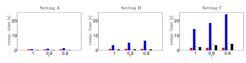
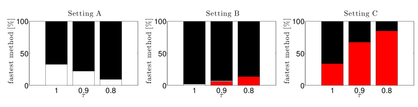
Figure 3: Empirical test on Setting A, B, and C for the methods CG-IRLS (blue), CG-IRLSm (white), IHT+CG-IRLSm (black), and IHT (red). Upper: Mean computational time. Center: Fastest method (in %). Lower: Failure rate (in %).

We conclude that CG-IRLSm and IHT+CG-IRLSm perform well for $\tau=1$ and for the problem dimension $N$ within the range of 1000 – 10000. They are even able to outperform IHT. However, by extrapolation of the numerical results IHT is expected to be faster for $N>10000$. (This is in compliance with the general folklore that first order methods should be preferred for higher dimension. However, as we will see in Subsection 5.3, a proper preconditioning of CG-IRLS-$\lambda$ will win over IHT for dimensions $N\geqslant 10^{5}$!) As soon as $N<1000$, direct methods such as Gaussian elimination are faster than CG, and thus, one should use standard IRLS with $\tau<1$.

Choice of $\beta$, maxiter_cg, and start_iht

The numerical tests in the previous paragraph were preceded by a careful and systematic investigation of the tuning of the parameters $\beta$, maxiter_cg, and start_iht. While we fixed start_iht to 100, 150, and 200 for Setting A, B, and C respectively to produce a good starting value, we tried $\beta\in\{1/N,0.01,0.1,0.5,0.75,1,1.5,2,5,10\}$, and $\texttt{maxiter\_cg}\in\{\lfloor m/8\rfloor,\lfloor m/12\rfloor,\lfloor m/16\rfloor\}$ for each setting. The results of this parameter sensitivity study can be summarized as follows:

• The best computational time is obtained for $\beta\sim 1$. In particular the computational time is not depending substantially on $\beta$ in this order of magnitude. More precisely, for CG-IRLS the choice of $\beta=0.5$ and for (IHT+)CG-IRLSm the choice of $\beta=2$ works best.

• The choice of maxiter_cg very much determines the tradeoff between failure and speed of the method. The value $\lfloor m/12\rfloor$ seems to be the best compromise. For a smaller value the failure rate becomes too high, for a larger value the method is too slow.

Phase transition diagrams.

Besides the empirical analysis of the speed of convergence, we also investigate the robustness of CG-IRLS with respect to the achievable sparsity level for exact recovery of $x^{*}$. Therefore, we fix $N=2000$ and we compute a phase transition diagram for IHT and CG-IRLS on a regular Cartesian $50\times 40$ grid, where one axis represents $m/N$ and the other represents $k/m$. For each grid point we plot the empirical success recovery rate, which is numerically realized by running both algorithms on 20 random trials. CG-IRLS or IHT is successful if it is able to compute a solution with a relative error of less than $1\text{\sc{e}-}4$ within 20 or 500 (outer) iterations respectively. Since we aim at simulating a setting in which the sparsity $k$ is not known exactly, we set the parameter $K=1.1\cdot k$ for both IHT and CG-IRLS. The interpolated plot is shown in Figure 4. It turns out that CG-IRLS has a significantly higher success recovery rate than IHT for less sparse solutions.

Figure 4: Phase transition diagrams of IHT and CG-IRLS for $N=2000$. The recovery rate is presented in grayscale values from 0% (white) up to 100% (black). As a reference, in the right subfigure, the 90% recovery rate level line of the CG-IRLS phase transition diagram is plotted to show more evidently the improved success rate of the latter algorithm.

5.3 Algorithm CG-IRLS-$\lambda$

Specific settings

We restrict the maximal number of outer iterations to 25. Furthermore, we modify (56), so that the CG-algorithm also stops as soon as $\left\|\rho^{n+1,i}\right\|_{\ell_{2}}\leqslant 1\text{\sc{e}-}16\cdot N^{3/2}m$. As soon as the residual undergoes this particular threshold, we call the CG solution (numerically) “exact”. The $\varepsilon$-update rule is extended by imposing the lower bound $\varepsilon^{n}=\varepsilon^{n}\vee\varepsilon^{\min}$ where $\varepsilon^{\min}=1\text{\sc{e}-}9$. Additionally we propose to choose $\varepsilon^{n+1}\leqslant 0.8^{n}\varepsilon^{n}$, which practically turns out to increase dramatically the speed of convergence. The summable sequence $(a_{n})_{n\in\mathbb{N}}$ in Theorem 4.1 is defined by setting $a_{n}=\sqrt{Nm}\cdot{10^{4}}\cdot(1/2)^{n}$. We split our investigation into a noisy and a noiseless setting.

For the noisy setting we set $\text{MSNR}=10$. According to birits09 ; candes2009 , we choose $\lambda=c\sigma\sqrt{m\log N}$ as a near-optimal regularization parameter, where we empirically determine $c=0.48$. Since we work with relatively large values of $\lambda$ in the regularized problem (49), we cannot use the synthesized sparse solution $x^{*}$ as a reference for the convergence analysis. Instead, we need another reliable method to compute the minimizer of the functional. In the convex case of $\tau=1$, this is performed by the well-known and fast algorithm FISTA beck09 , which shall also serve as a benchmark for the speed analysis. In the non-convex case of $\tau<1$, there is no method which guarantees the computation of the global minimizer, thus, we have to omit a detailed speed-test in this case. However, we describe the behavior of Algorithm CG-IRLS-$\lambda$ for $\tau$ changing.

If the problem is noiseless, i.e., $e=0$, the solution $x^{\lambda}$ of (49) converges to the solution of (1) for $\lambda\rightarrow 0$. Thus, we choose $\lambda=m\cdot 1\text{\sc{e}-}8$, and assume the synthesized sparse solution $x^{*}$ as a good proxy for the minimizer and a reference for the convergence analysis. (Actually, this can also be seen the other way around, i.e., we use the minimizer $x^{\lambda}$ of the regularized functional to compute a good approximation to $x^{*}$.) It turns out that for $\lambda\approx 0$, as we comment below in more detail, FISTA is basically of no use.

CG-IRLS-$\lambda$ vs. IRLS-$\lambda$

As in the previous subsection, we first show that the CG-method within IRLS-$\lambda$ leads to significant improvements in terms of the computational speed. Therefore we choose a noisy trial of Setting B, and compare the computational time of the methods IRLS-$\lambda$, CG-IRLS-$\lambda$, and FISTA. The result is presented on the left plot of Figure 5. We observe, that CG-IRLS-$\lambda$ computes the first iterations in much less time than IRLS-$\lambda$, but due to bad conditioning of the inner CG problems it performs much worse afterwards. Furthermore, as may be expected, the algorithm is not suitable to compute a highly accurate solution. For the computation of a solution with a relative error in the order of $1\text{\sc{e}-}3$, CG-IRLS-$\lambda$ outperforms FISTA. FISTA is able to compute highly accurate solutions, but a solution with a relative error of $1\text{\sc{e}-}3$ should be sufficient in most applications because the goal in general is not to compute the minimizer of the Lagrangian functional but an approximation of the sparse signal.

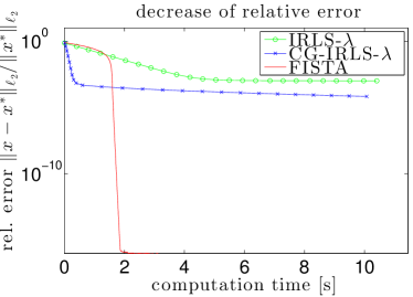
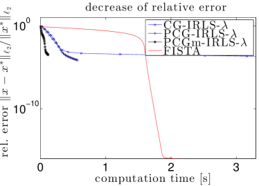
Figure 5: Single trial of Setting B. Left: Relative error plotted against the computational time for IRLS-$\lambda$ (light green, $\circ$), CG-IRLS-$\lambda$ (blue, $\times$), and FISTA (red, $-$). Right: Relative error plotted against computational time for CG-IRLS-$\lambda$ (blue, $\times$), PCG-IRLS-$\lambda$ (dark blue, $+$), PCGm-IRLS-$\lambda$ (black, $*$), and FISTA (red, $-$).

Modifications to CG-IRLS-$\lambda$

To further decrease the computational time of CG-IRLS-$\lambda$, we propose the following modifications:

1. To overcome the bad conditioning in the CG loop, we precondition the matrix $A_{n}=\Phi^{*}\Phi+\operatorname*{diag}\left[\lambda\tau w_{j}^{n}\right]_{j=1}^{N}$ by means of the Jacobi preconditioner, i.e., we pre-multiply the linear system by the inverse of its diagonal, $\left(\operatorname*{diag}A_{n}\right)^{-1}$, which is a very efficient operation in practice.

2. We introduce the parameter maxiter_cg which defines the maximal number of inner CG iterations and is set to the value $\texttt{maxiter\_cg}=4$ in the following.

The algorithm with modification (i) is called PCG-IRLS-$\lambda$, and the one with modification (i) and (ii) PCGm-IRLS-$\lambda$. We run these algorithms on the same trial of Setting B as in the previous paragraph. The respective result is shown on the right plot of Figure 5. This time, preconditioning effectively yields a strong decrease of computational time, especially in the final iterations where $A_{n}$ is badly conditioned. Furthermore, modification (ii) importantly increases the performance of the proposed algorithm also in the initial iterations. However, again we have to take into consideration that we may violate the assumptions of Theorem 4.1 so that convergence is not guaranteed anymore and failure rates might potentially increase. In the two paragraphs below that are entitled Empirical test on computational time and failure rate with noisy/noiseless data, we present simulations on noisy and noiseless data, which give a more precise picture of the speed and failure rate of the previously introduced methods in comparison to FISTA and IHT.

We investigate the influence of the tolerance $\textnormal{tol}_{n}$ and the number of (inner) iterations of the CG procedure performed along the IRLS iterations in Figure 6 for CG-IRLS-$\lambda$, PCG-IRLS-$\lambda$, and PCGm-IRLS-$\lambda$. We see that the methods do not differ much in terms of the tolerance. In particular CG-IRLS-$\lambda$ and PCG-IRLS-$\lambda$ have nearly the same sequence of $\textnormal{tol}_{n}$, however, due to the bad conditioning, the number of inner CG iterations tremendously increases with growing number of outer IRLS iterations in CG-IRLS-$\lambda$. In contrast, the number of inner CG iterations in PCG-IRLS-$\lambda$ stays very low. A bound on the CG iterations of $\texttt{maxiter\_cg}=4$ does only very slightly change the behavior of $\textnormal{tol}_{n}$ in PCGm-IRLS-$\lambda$ and leads to a further advantage in the computational time, as can be seen in Figure 5.

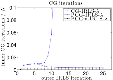
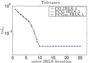
Figure 6: Single trial of Setting B. Left: Number of CG iterations (divided by $N$) plotted against the outer iteration number for CG-IRLS-$\lambda$ (blue, $\times$), PCG-IRLS-$\lambda$ (dark blue, $+$), PCGm-IRLS-$\lambda$ (black, $*$). Right: Tolerance $\textnormal{tol}_{n}$ plotted against the outer iteration number for the same algorithms.

Empirical test on computational time and failure rate with noisy data

In the previous paragraph, we observed that the CG-IRLS-$\lambda$ methods are only computing efficiently solutions with a low relative error. Thus we now focus on this setting and compare the three methods PCG-IRLS-$\lambda$, PCGm-IRLS-$\lambda$, and FISTA with respect to their computational time and failure rate in recovering solutions with a relative error of $1\text{\sc{e}-}1$, $1\text{\sc{e}-}2$, and $1\text{\sc{e}-}3$. We only consider the convex case $\tau=1$. Similarly to the procedure in Section 5.2, we run these algorithms on 100 trials for each setting with the respectively chosen values of $\lambda$. In Figure 7 the upper bar plot shows the result for the mean computational time and the lower stacked bar plot shows how often a method was the fastest one. We do not present a plot of the failure rate since none of the methods failed at all. By means of the plots, we demonstrate that both PCG-IRLS-$\lambda$, and PCGm-IRLS-$\lambda$ are faster than FISTA, while PCGm-IRLS-$\lambda$ always performs best.

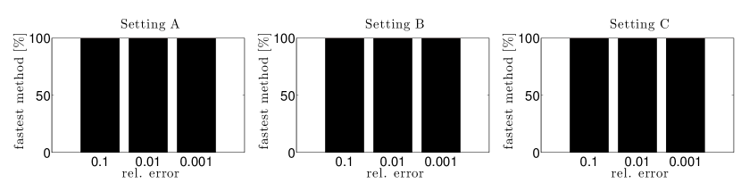
Figure 7: Empirical test on Setting A, B, and C for the methods PCG-IRLS-$\lambda$ (blue), PCGm-IRLS-$\lambda$ (black), and FISTA (red). Upper: Mean computational time. Lower: Fastest method (in %).

Empirical test on computational time and failure rate with noiseless data

In the noiseless case, we compare the computational time of FISTA and PCGm-IRLS-$\lambda$ to IHT and IHT+CG-IRLSm. We set $\texttt{maxiter\_cg}=40$ for PCGm-IRLS-$\lambda$. In a first test, we run these algorithms on one trial of Setting A, and C respectively, and plot the results in Figure 8.

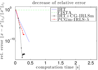
Figure 8: Left: Setting A. Right: Setting C. Comparison of IHT (blue, $-$), FISTA (green, $--$), IHT+CG-IRLSm (black, $*$), and PCGm-IRLS-$\lambda$ (red, $\times$).

As already mentioned, FISTA is not suitable for small values of $\lambda$ on the order of $m\cdot 1\text{\sc{e}-}8$ and converges then extremely slowly, but PCGm-IRLS-$\lambda$ can compete with the remaining methods. IHT+CG-IRLSm is in some settings able to outperform IHT, at least when a high accuracy is needed. PCGm-IRLS-$\lambda$ is always at least as fast as IHT with increasing relative performance gain for increasing dimensions. This observation suggests the conjecture that PCGm-IRLS-$\lambda$ provides the fastest method also in rather high dimensional problems. To validate this hypothesis numerically, we introduce two new high dimensional settings (to reach higher dimensionalities and retaining low computation times for the extensive tests it is again very beneficial to use the real cosine transform as a model for $\Phi$):

	Setting D	Setting E
N	100000	1000000
m	40000	400000
k	1500	15000
K	2500	25000

We run the most promising algorithms IHT and PCGm-IRLS-$\lambda$ on a trial of the large scale settings D and E. The result, which is plotted in Figure 9, shows that PCGm-IRLS-$\lambda$ is able to outperform IHT in these settings unless one requires an extremely low relative error ($\leqslant 1\text{\sc{e}-}8$), because of the error saturation effect. We confirm this outcome in a test on 100 trials for Setting D and E and present the result in Figure 10.

Figure 9: Left: Setting D. Right: Setting E. Comparison of IHT (blue, $-$), and PCGm-IRLS-$\lambda$ (red, $\times$).

Figure 10: Empirical test on the mean computational time of Setting D and E for the methods IHT (blue), and PCGm-IRLS-$\lambda$ (red).

Dependence on $\tau$.

In the last experiment of this paper, we are interested in the influence of the parameter $\tau$. Of course, changing $\tau$ also means modifying the problem resulting in a different minimizer. Due to non-convexity also spurious local minimizers may appear. Therefore, we do not compare the speed of the method to FISTA. In Figure 11, we show the performance of Algorithm PCGm-IRLS-$\lambda$ for a single trial of Setting C and the parameters $\tau\in\{1,0.9,0.8,0.7\}$ for the noisy and noiseless setting. As reference for the error analysis, we choose the sparse synthetic solution $x^{*}$, which is actually not the minimizer here.

In both the noisy and noiseless setting, using a parameter $\tau<1$ improves the computational time of the algorithm. In the noiseless case, $\tau=0.9$ seems to be a good choice, smaller values do not improve the performance. In contrast, in the noisy setting the computational time decreases with decreasing $\tau$.

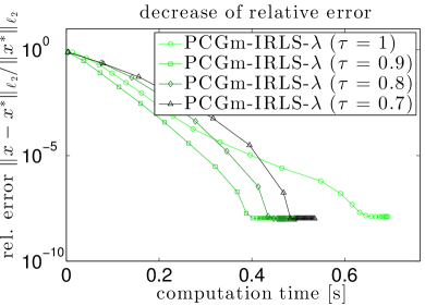
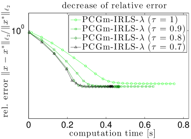
Figure 11: Results of Algorithm PCGm-IRLS-$\lambda$ for a single trial of Setting C for different values of $\tau$ with noise (right) and without noise (left).

Appendix A Proof of Lemma 10

“$\Rightarrow$”(in the case $0<\tau\leqslant 1$)
Let $x=x^{{\varepsilon},1}$ or $x\in\mathcal{X}_{{\varepsilon},\tau}(y)$, and $\eta\in\mathcal{N}_{\Phi}$ arbitrary. Consider the function

$$G_{{\varepsilon},\tau}(t)\mathrel{\mathop{:}}=f_{{\varepsilon},\tau}\left(x+t\eta\right)-f_{{\varepsilon},\tau}\left(x\right)$$

with its first derivative

$$G^{\prime}_{{\varepsilon},\tau}(t)=\tau\sum\limits_{i=1}^{N}\frac{x_{i}\eta_{i}+t\eta_{i}^{2}}{\left[|x_{i}+t\eta_{i}|^{2}+{\varepsilon}^{2}\right]^{\frac{2-\tau}{2}}}.$$

Now $G_{{\varepsilon},\tau}(0)=0$ and from the minimization property of $f_{{\varepsilon},\tau}(x)$, $G_{{\varepsilon},\tau}(t)\geq 0$. Therefore,

$$0=G^{\prime}_{{\varepsilon},\tau}(0)=\sum\limits_{i=1}^{N}\frac{x_{i}\eta_{i}}{\left[x_{i}^{2}+{\varepsilon}^{2}\right]^{\frac{2-\tau}{2}}}=\left\langle x,\eta\right\rangle_{\hat{w}(x,{\varepsilon},\tau)}.$$

“$\Leftarrow$”(only in the case $\tau=1$)
Now let $x\in\mathcal{F}_{\Phi}(y)$ and $\left\langle x,\eta\right\rangle_{\hat{w}(x,{\varepsilon},1)}=0$ for all $\eta\in\mathcal{N}_{\Phi}$. We want to show that $x$ is the minimizer of $f_{{\varepsilon},1}$ in $\mathcal{F}_{\Phi}(y)$. Consider the convex univariate function $g(u)\mathrel{\mathop{:}}=[u^{2}+{\varepsilon}^{2}]^{1/2}$. For any point $u_{0}$ we have from convexity that

$$[u^{2}+{\varepsilon}^{2}]^{1/2}\geqslant[u_{0}^{2}+{\varepsilon}^{2}]^{1/2}+[u_{0}^{2}+{\varepsilon}^{2}]^{-1/2}u_{0}(u-u_{0})$$

because the right-hand-side is the linear function which is tangent to $g$ at $u_{0}$. It follows, that for every point $v\in\mathcal{F}_{\Phi}(y)$ we have

$$f_{{\varepsilon},1}(v)\geqslant f_{{\varepsilon},1}(x)+\sum\limits_{i=1}^{N}{[x_{i}^{2}+{\varepsilon}^{2}]^{-1/2}x_{i}(v_{i}-x_{i})}=f_{{\varepsilon},1}(x)+\left\langle x,v-x\right\rangle_{\hat{w}(x,{\varepsilon},1)}=f_{{\varepsilon},1}(x),$$

where we have used the orthogonality condition and the fact that $(v-x)\in\mathcal{N}_{\Phi}$. Since $v$ was chosen arbitrarily, $x=x^{{\varepsilon},1}$ as claimed.

- (1) Beck, A., Teboulle, M.: A fast iterative shrinkage-thresholding algorithm for linear inverse problems. SIAM J. Imaging Sci. 2(1), 183–202 (2009). DOI 10.1137/080716542. URL http://dx.doi.org/10.1137/080716542
- (2) Bickel, P., Ritov, Y., Tsybakov, A.: Simultaneous analysis of lasso and Dantzig selector. Ann. Statist. 37(4), 1705–1732 (2009)
- (3) Blumensath, T., Davies, M.E.: Iterative hard thresholding for compressed sensing. Appl. Comput. Harmon. Anal. 27(3), 265–274 (2009). DOI 10.1016/j.acha.2009.04.002. URL http://dx.doi.org/10.1016/j.acha.2009.04.002
- (4) Bredies, K., Lorenz, D.A.: Minimization of non-smooth, non-convex functionals by iterative thresholding. J. Optim. Theory Appl. 165, 78–112 (2015)
- (5) Candès, E.J., J., Tao, T., Romberg, J.: Robust uncertainty principles: exact signal reconstruction from highly incomplete frequency information. IEEE Trans. Inform. Theory 52(2), 489–509 (2006)
- (6) Candès, E.J., Plan, Y.: Near-ideal model selection by minimization. Ann. Statist. 37(5A), 2145–2177 (2009). DOI 10.1214/08-AOS653. URL http://dx.doi.org/10.1214/08-AOS653
- (7) Candès, E.J., Tao, T.: Near optimal signal recovery from random projections: universal encoding strategies? IEEE Trans. Inform. Theory 52(12), 5406–5425 (2006)
- (8) Chafai, D., Guédon, O., Lecué, G., Pajor, A.: Interactions between Compressed Sensing, Random Matrices and high Dimensional Geometry. Soc. Math. France, Paris (2012)
- (9) Chambolle, A., Lions, P.L.: Image recovery via total variation minimization and related problems. Numer. Math. 76(2), 167–188 (1997). DOI 10.1007/s002110050258. URL http://dx.doi.org/10.1007/s002110050258
- (10) Chartrand, R.: Exact reconstruction of sparse signals via nonconvex minimization. Signal Processing Letters, IEEE 14(10), 707–710 (2007). DOI 10.1109/LSP.2007.898300
- (11) Chartrand, R., Staneva, V.: Restricted isometry properties and nonconvex compressive sensing. Inverse Problems 24(3), 035,020, 14 (2008). DOI 10.1088/0266-5611/24/3/035020. URL http://dx.doi.org/10.1088/0266-5611/24/3/035020
- (12) Chartrand, R., Yin, W.: Iteratively reweighted algorithms for compressive sensing. In: Acoustics, Speech and Signal Processing, 2008. ICASSP 2008. IEEE International Conference on, pp. 3869–3872 (2008). DOI 10.1109/ICASSP.2008.4518498
- (13) Chen, S.S., Donoho, D.L., Saunders, M.A.: Atomic decomposition by Basis Pursuit. SIAM J. Sci. Comput. 20(1), 33–61 (1999)
- (14) Cline, A.K.: Rate of convergence of Lawson’s algorithm. Math. Comp. 26, 167–176 (1972)
- (15) Cohen, A., Dahmen, W., DeVore, R.A.: Compressed sensing and best -term approximation. J. Amer. Math. Soc. 22(1), 211–231 (2009)
- (16) Daubechies, I., DeVore, R., Fornasier, M., Güntürk, C.: Iteratively re-weighted least squares minimization for sparse recovery. Comm. Pure Appl. Math. 63(1), 1–38 (2010)
- (17) Dirksen, S., Lecu’e, G., Rauhut, H.: On the gap between RIP-properties and sparse recovery conditions. Preprint ArXiv:1504.05073 (2015)
- (18) Donoho, D.L.: Compressed sensing. IEEE Trans. Inform. Theory 52(4), 1289–1306 (2006)
- (19) Fornasier, M., Rauhut, H., Ward, R.: Low-rank matrix recovery via iteratively reweighted least squares minimization. SIAM J. Optim. 21(4), 1614–1640 (2011). DOI 10.1137/100811404. URL http://dx.doi.org/10.1137/100811404
- (20) Foucart, S., Rauhut, H.: A Mathematical Introduction to Compressive Sensing. New York, NY: Birkhäuser/Springer (2013). DOI 10.1007/978-0-8176-4948-7
- (21) Gorodnitsky, I.F., Rao, B.D.: Sparse signal reconstruction from limited data using FOCUSS: a recursive weighted norm minimization algorithm. IEEE Transactions on Signal Processing 45(3), 600–616 (1997)
- (22) Gribonval, R., Nielsen, M.: Sparse representations in unions of bases. IEEE Trans. Inform. Theory 49(12), 3320–3325 (2003)
- (23) Han, W., Jensen, S., Shimansky, I.: The Kačanov method for some nonlinear problems. Appl. Numer. Math. 24(1), 57–79 (1997)
- (24) Hestenes, M.R., Stiefel, E.: Methods of Conjugate Gradients for Solving Linear Systems. Journal of Research of the National Bureau of Standards 49(6), 409–436 (1952)
- (25) Hollanda, P.W., Welsch, R.E.: Robust regression using iteratively reweighted least-squares. Communications in Statistics - Theory and Methods 6(9), 813–827 (1977)
- (26) Ito, K., Kunisch, K.: A variational approach to sparsity optimization based on Lagrange multiplier theory. Inverse Problems 30(1), 015,001, 23 (2014). DOI 10.1088/0266-5611/30/1/015001. URL http://dx.doi.org/10.1088/0266-5611/30/1/015001
- (27) Jacobs, D.A.H.: A generalization of the conjugate-gradient method to solve complex systems. IMA journal of numerical analysis 6(4), 447–452 (1986)
- (28) Kabanava, M., Rauhut, H.: Analysis -recovery with frames and Gaussian measurements. Acta Appl. Math. (to appear)
- (29) King, J.T.: A minimal error conjugate gradient method for ill-posed problems. J. Optim. Theory Appl. 60, 297–304 (1989). URL http://dx.doi.org/10.1007/BF00940009
- (30) Krahmer, F., Mendelson, S., Rauhut, H.: Suprema of chaos processes and the restricted isometry property. Comm. Pure Appl. Math. 67(11), 1877–1904 (2014)
- (31) Lai, M.J., Xu, Y., Yin, W.: Improved iteratively reweighted least squares for unconstrained smoothed minimization. SIAM Journal on Numerical Analysis 51(2), 927–257 (2013)
- (32) Lawson, C.L.: Contributions to the Theory of Linear Least Maximum Approximation. Ph.D. thesis. University of California, Los Angeles (1961)
- (33) Lecuè, G., Mendelson, S.: Sparse recovery under weak moment assumptions. J. Europ. Math. Soc. (to appear)
- (34) Nocedal, J., Wright, S.: Conjugate Gradient Methods, pp. 101–134. Springer Series in Operations Research and Financial Engineering. Springer (2006)
- (35) Ochs, P., Dosovitskiy, A., Brox, T., Pock, T.: On iteratively reweighted algorithms for nonsmooth nonconvex optimization in computer vision. SIAM J. Imaging Sci. 8(1), 331–372 (2015). DOI 10.1137/140971518
- (36) Osborne, M.R.: Finite algorithms in optimization and data analysis. Wiley Series in Probability and Mathematical Statistics: Applied Probability and Statistics. John Wiley & Sons, Ltd., Chichester (1985)
- (37) Quarteroni, A., Sacco, R., Saleri, F.: Numerical Mathematics. Texts in Applied Mathematics Series. Springer-Verlag GmbH (2000). URL http://books.google.de/books?id=YVpyyi1M7vUC
- (38) Ramlau, R., Zarzer, C.A.: On the minimization of a Tikhonov functional with a non-convex sparsity constraint. Electron. Trans. Numer. Anal. 39, 476–507 (2012)
- (39) Rauhut, H.: Compressive sensing and structured random matrices. In: M. Fornasier (ed.) Theoretical foundations and numerical methods for sparse recovery, Radon Series Comp. Appl. Math., vol. 9, pp. 1–92. deGruyter (2010)
- (40) Rudelson, M., Vershynin, R.: On sparse reconstruction from Fourier and Gaussian measurements. Comm. Pure Appl. Math. 61, 1025–1045 (2008)
- (41) Rudin, L., Osher, S., Fatemi, E.: Nonlinear total variation based noise removal algorithms. Physica D 60(1-4), 259–268 (1992)
- (42) Vogel, C.R., Oman, M.E.: Fast, robust total variation-based reconstruction of noisy, blurred images. IEEE Trans. Image Process. 7(6), 813–824 (1998). DOI 10.1109/83.679423
- (43) Voronin, S.: Regularization of linear systems with sparsity constraints with applications to large scale inverse problems. Ph.D. thesis, Applied and Computational Mathematics Department, Princeton University (2012)
- (44) Voronin, S., Daubechies, I.: An Iteratively Reweighted Least Squares Algorithm for Sparse Regularization. arXiv:1511.08970 [math] (2015)
- (45) Zarzer, C.A.: On Tikhonov regularization with non-convex sparsity constraints. Inverse Problems 25(2), 025,006, 13 (2009). DOI 10.1088/0266-5611/25/2/025006. URL http://dx.doi.org/10.1088/0266-5611/25/2/025006