Controlling contagious processes
on temporal networks via adaptive rewiring

Abstract

We consider recurrent contagious processes on a time-varying network. As a control procedure to mitigate the epidemic, we propose an adaptive rewiring mechanism for temporary isolation of infected nodes upon their detection. As a case study, we investigate the network of pig trade in Germany. Based on extensive numerical simulations for a wide range of parameters, we demonstrate that the adaptation mechanism leads to a significant extension of the parameter range, for which most of the index nodes (origins of the epidemic) lead to vanishing epidemics. Furthermore the performance of adaptation is very heterogeneous with respect to the index node. We quantify the success of the proposed adaptation scheme in dependence on the infectious period and detection times. To support our findings we propose a mean-field analytical description of the problem.

I Introduction

Recently the availability of data on host mobility and contact patterns of high resolution offers many opportunities for the design of new tools and approaches for modeling and control of epidemic spread DAN13a ; BAR14 ; STE11 ; SCH13a ; BEL11 . To exploit these versatile concepts of complex networks research, hosts or their spatial aggregations are considered as nodes and host contacts or their relocations as edges. Very frequently the edges are not static, but changing with time. If dynamical processes on networks possess a characteristic time scale much faster than the time scale of the changing edges, a static, quenched approximation of the topology may be sufficient. However if the time scale of the process is comparable with the time scale of the network change, a more sophisticated concept of time-varying or temporal networks is required, because static approximation might violate the causality principle CAS12 ; LEN13 ; HOL12 ; SCH14k ; KON12a ; KIV12 ; BAJ12 ; VOL09 ; VAL15a . Although for static networks a variety of surveillance and control approaches were proposed based on various network measures such as node degree, betweenness centrality etc. SCH11h , control concepts for temporal networks are still missing. The previous studies on this topic were devoted mostly to targeted vaccination policies LEE12 ; STA13 ; BUE13 ; LIU14 ; RIZ14 ; TAN11a and general controllability questions POS14 ; SEL14 . Furthermore, an adaptation of edges was proposed to mitigate the spread in static networks GRO06b ; GRO08a ; SHA08a ; VAN10a ; YAN15 and by random rewiring, a co-evolution of the network and the spreading was implemented to avoid infected nodes. However, there have been no studies combining the adaptation approach of epidemic control with intrinsic temporal changes of the underlying network structure.

In this paper, we propose an adaptive non-targeted control mechanism for spreading processes on temporal networks and assess its effectiveness. We consider a deterministic recurrent contagious dynamics similar to a susceptible-infected-susceptible (SIS) model. In our model, susceptible nodes, after contact with an infected node, become infected and after a fixed time $\kappa$ they become again susceptible to the disease. We assume that the nodes are screened for infection, but the information whether or not a node is infected is available only after some detection time $\delta$. One can interpret the detection time $\delta$ as a time required to reliably detect the disease (also called window period BRO04 ) or a time the disease needs to manifest itself (incubation time) and be diagnosed. After the detection we apply adaptation rules, rewiring our system in a way to avoid edges emanating from the detected infected nodes. This results effectively in a temporary quarantine of the infected nodes..

We pursue the question, if the interplay between the intrinsic dynamics of a temporal network and adaptation rules leads to a substantial improvement of the disease mitigation. In contrast to a range of studies considering targeted intervention measures, we apply control measures to all infected nodes, after they are detected as those. Our approach can be easily supplemented by targeted interventions as well, where only some fraction of specific nodes is controled.

This paper is structured as follows: First, we introduce the empirical dataset and outline our approach to adaptive epidemic control. Then, we present results on the mitigation strategy and discuss their implications. Finally, we summarize our findings and provide an outlook on further research directions.

II Methods and Dataset

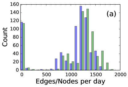
Figure 2: (a) Histogram of the number of active edges (blue) and nodes (green) (daily resolution). (b) Distribution of the size of out-components for all nodes. The inset shows the same on a semi-log scale.

The empirical temporal network investigated in our study is extracted from the database on pig trade in Germany HI-Tier (See also Data Accessibility Section). We use an excerpt from this animal (pig) trade network with 15,569 agricultural premises (nodes) over a period of observation of 2 years (daily resolution), which consists of 748,430 trade events (links). All premises have been anonymized for the study. On average day (except Sunday) the network contains 1220 nodes with 1141 edges as depicted in Fig. 2(a) (Supplementary Material). We observe a non-uniform activity with respect to the day of the week (see Supplementary Material, Fig. 1): on average, we find 1346 nodes with 1258 edges on a working day and 932 or 43 nodes with 844 or 27 edges on Saturday and Sunday, respectively. This reduced activity on the weekend is clearly visible in Fig. 2(a) (Supplementary Material). The trade flow is directed: from source nodes (piglet producers) to sink nodes (slaughter houses). There are 291 sinks, which only have in-coming links, but no out-going links, and 5,504 sources with only in-coming links. For fuhrer details on basic network characteristics, see Tab. 1 in Supplementary Material.

The considered network also possesses a strong heterogeneity with respect to the size of out-components as shown in Fig 2(b) (Supplementary Material). The out-component of a node is defined as the number of nodes that could be infected in a worst-case SI (susceptible-infected) epidemic scenario with an outbreak originating from that particular node upon its first occurrence. For this worst case, we assume the infinite infectious period and consider an SI epidemic following the directed, temporal links during the whole observation time. The distribution of the out-components peaks around 6,000 nodes, which corresponds to 40% of the network. We also find many cases, where an outbreak immediately stops and the length of the respective epidemic path is short. Among these nodes are the above-mentioned sink nodes.

Therefore, it can be expected that the prevalence, i.e. the total number of infected nodes at a given point in time, strongly depends on the outbreak origin, and a surveillance strategy that randomly selects nodes for screening will not be effective. In addition, for finite infectious periods, the day of first infection is important as has been shown in Ref. KON12a .

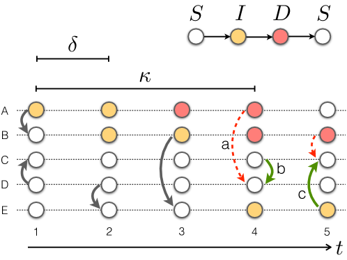
Figure 1: (Color online) Infection model and adaptation mechanism. Nodes are arranged vertically with links between them for each day. Nodes can be in three states: susceptible, $S$ (empty circles), undetected infected, $I$ (yellow), and detected infected, $D$ (red). After $\delta$ days, infected nodes are detected and for $t\in[t^{\star}+\delta,t^{\star}+\kappa]$ – with $t^{\star}$ being the time of infection – all out-going links from the detected nodes (red) are randomly rewired to other susceptible or undetected nodes as starting point, e.g. the link a is destroyed and instead the link b is created. Note that a newly created links might spread the disease as well. E.g. on day 5 the green arrow might point from the undetected infected node E to the node C (link c) spreading the disease. After $\kappa$ days, infected nodes become susceptible again. Parameters: $\delta=2$ d, $\kappa=4$ d.

In our simulations on this real-world temporal network, we consider a deterministic recurrent epidemic of an SIS type. Note that SIS epidemics on temporal networks without adaptation have been investigated in Ref. ROC13 . The spreading process is deterministic in the following sense: every time a trade event from an infected to a susceptible premise takes place, the susceptible one becomes infected with probability 1. In other words, we consider diseases with high infectiousness and thus a worst-case scenario for a spreading process. More precisely, nodes can be susceptible ($S$), infected undetected ($I$), or infected detected ($D$) as depicted in Fig 1. After detection time $\delta$, infected nodes are detected and according to our control strategy, all of their out-going links are rewired to start at other susceptible or infected, but not yet detected nodes chosen at random. Thus, we isolate the detected infectious nodes or place them under quarantine. The total period of infection is denoted by $\kappa\geq\delta$. Note that nodes, which are infected, but not yet detected, take part in the rewiring and thus, eventually increase the risk of receiving nodes. See, for instance, the newly formed (green) link from node E to C at $t=5$ d in Fig. 1. The proposed adaptation scheme can be easily implemented for SIR models, where the infected nodes become immune, that is, recovered, after the infection period. This would, however, considerably reduce the pool of available nodes over the course of the available observation period.

III Results and discussions

In this section, we discuss the main findings based on the model and data described above. A typical evolution of the number of infected nodes (prevalence) is shown in Fig. 2 for an arbitrary starting node and the infectious period $\kappa=45$ d. For a free-running sustained disease, i.e. without network adaptation or other measures of mitigation ($\kappa=\delta$), one can observe that the prevalence fluctuates around a constant endemic level after a short transient period as shown by the blue curve. The effect of network adaptation manifests itself either in a reduction of this endemic prevalence level (orange curve in Fig. 2, where network adaptation takes place after $\delta=25$ d) or termination of an outbreak as shown by the red curve for $\delta=13$ d. This shows that the considered adaptation scheme can substantially limit the spreading potential of an outbreak. This is also confirmed by the mean-field approximation (Section IV).

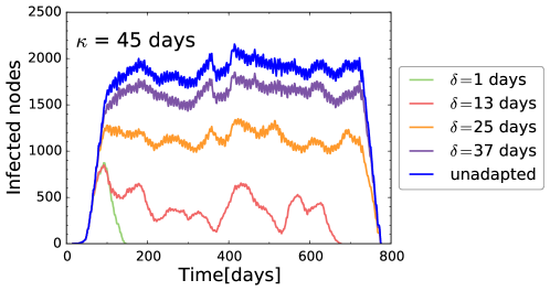
Figure 2: (Color online) Typical time course of an epidemic. Prevalence (number of infected nodes, daily resolution) for a fixed infectious period $\kappa=30$ d and different detection times $\delta$. Whereas unadapted epidemic with $\delta=\kappa$ (blue curve), adapted epidemics with $\delta=37$ d (purple), $\delta=25$ d (orange) are persistent, adapted epidemics with $\delta=13$ d (red) and $\delta=1$ d (green) die out before the end of the observation.

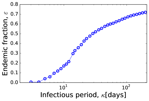
Figure 3: (Color online) Endemic fraction $\varepsilon$ in dependence on the infectious time $\kappa$ without control adaptive rewiring.

In general, different nodes as origins of infection lead to different outcomes, some of them lead to epidemics and some do not. Note that we always start our simulation with just one origin (or index) node infected. In order to evaluate the influence of every possible node as an origin of infection, we scan the whole network by separately considering each node as the origin of an outbreak upon the node’s first appearance in the dataset. Technically we define epidemics as persistent if after 700 days (at the end of the maximal observation time) there still exists a non-zero prevalence in the system. Therefore we define the endemic fraction or the probability of an epidemic to be sustained as the fraction of index nodes leading to persistent epidemics

$$\varepsilon=\frac{N_{\text{endemic}}}{N_{\text{total}}},$$ (1)

where $N_{\text{total}}$ is the total number of origin nodes and and $N_{\text{endemic}}$ is the number of origin nodes leading to persistent epidemics. Without adaptation, $\varepsilon$ increases with infectious period $\kappa$ (Fig. 3). Only for very small infectious periods ($\kappa\leq 3$ d) there is an almost vanishing endemic fraction due to the low frequency of network contacts. Values larger than $10$% are found for infectious periods larger than $5$ d. The highest endemic fraction in our system is around $70\%$ for $\kappa=200$ d. The considered $\kappa$-values fall in the biologically plausible range including bacterial diseases such as hemorrhagic diarrhea caused by E. Coli with animals carrying the disease up to 2 months COR04 .

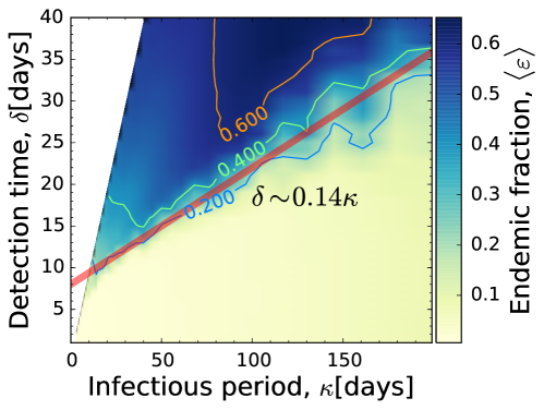
Figure 4: (Color online) Dependence of the endemic fraction $\varepsilon$ on the infectious period $\kappa$ and detection time $\delta$. In the region below the red line ($\delta\sim 0.14\kappa$) the persistence fraction is less than $10\%$.

Besides the infectious period $\kappa$ the adaptation introduces an additional time scale — the detection time $\delta$. The dependence of the endemic fraction $\epsilon$ in $(\kappa,\delta)$-parameter space is presented in Fig. 4. The uncontrolled case of Fig. 3 can be retrieved for $\delta=\kappa$. We find that the (almost) disease-free region of small $\varepsilon$ becomes significantly larger than in the uncontrolled case, where the vanishing prevalence was observed for small $\kappa\leq 3$. Due to the adaptation, the persistence fraction remains less than $10\%$ for parameter values below the red line $\delta\approx 0.14\kappa+\text{const}$.

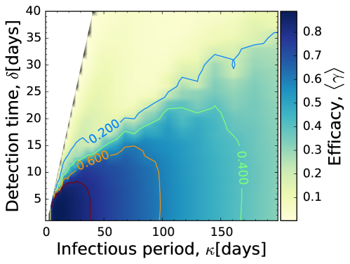
Figure 7: Prevalence reduction $\varepsilon$ in dependence on both infectious period and detection time.

The behavior of the persistence fraction is also shown in Figs. 7(a) and (b) (Supplementary Material), which shows the persistence fraction $\varepsilon$ for fixed $\delta$ or $\kappa$, i. e., horizontal or vertical sections through Fig. 4, respectively. In Fig. 7(a) (Supplementary Material) we observe that in most cases for a fixed detection time the persistence fraction, starting from high values, increases intitially to eventually decrease with the infectious period $\kappa$. In Fig. 7(b) we see that for fixed infectious period $\kappa$ the endemic fraction monotonically increases with the detection time $\delta$.

For recurrent epidemics like an SIS process, the impact of the mitigation strategy by rewiring strongly depends on the node, from which the outbreaks originates, i.e. the index node. This heterogeneity of the prevalence is the direct implication of the heterogeneity in the out-components (cf. Fig 2, Supplementary Material). The existence of clusters of nodes with similar prevalence values and adaptation properties is consistent with the existence of clusters of nodes with similar invasion routes as reported in Ref. BAJ12 . There are subsets of index nodes, belonging to the same cluster, which are most responsive to adaptation. This knowledge can be exploited to target those nodes with high priority, if resources for disease control are sparse. To quantify the effect of adaptation on prevalence reduction for persistent epidemics, we define the efficacy as

$$\gamma=\frac{\left(I_{\infty}-I^{*}_{\infty}\right)}{I_{\infty}},$$ (2)

where $I_{\infty}$ and $I^{*}_{\infty}$ denote the prevalence in the unadapted and adapted cases, respectively. Figure 5 (Supplementary Material) shows the influence of the index nodes and their impact on the success of the control measured in terms of the efficacy $\gamma$ for a fixed infectious period $\kappa=28$ d and different detection times $\delta$. For small $\delta$, we find the efficacy peaked at 90%. As the detection time becomes larger, the control becomes less effective indicated by smaller prevalence reduction. The mean efficacy averaged over all nodes as starting points is presented in Fig 8 in Supplementary Material. To characterize the heterogeneity of the distribution of the $\gamma$ values shown in Fig. 5 (Supplementary Material), we also compute its entropy. Its dependence on the infectious period and detection time is presented in Fig. 9 (Supplementary Material).

IV Mean-field Description

We approximate the deterministic dynamics on a temporal network described in Section II(See Fig. 1) with the following system of stochastic reactions

$$S+I \stackrel{{\scriptstyle\alpha}}{{\rightarrow}} 2I$$

$$S+D \stackrel{{\scriptstyle\alpha^{\prime}}}{{\rightarrow}} 2I$$

$$I \stackrel{{\scriptstyle\nu}}{{\rightarrow}} D$$

$$D \stackrel{{\scriptstyle\mu}}{{\rightarrow}} S.$$

The first reaction describes the usual infection of a susceptible by an infective with the infection rate $\alpha$ which in the deterministic case could correspond to the average daily out-degree of a node $\alpha\sim\langle k_{\rm out}\rangle$. The second reaction corresponds to the effective force of infection due to the occasional rewiring to infected nodes (See Fig. 1, link $\bf c$) which reads $\alpha^{\prime}SD$ with the effective infection rate $\alpha^{\prime}=\alpha I/(I+S)$. The third reaction represent the detection with the rate $\nu\sim 1/\delta$. And the last one the recovery with the rate $\mu\sim 1/(\kappa-\delta)$. Using the fractions $j=I/N$, $s=S/N,$ and $z=D/N$, the corresponding set of differential equations reads

$$\frac{dj}{dt} = \alpha\left(1+\frac{z}{j+s}\right)js-\nu j,$$

$$\frac{ds}{dt} = -\alpha\left(1+\frac{z}{j+s}\right)js+\mu z,$$

$$\frac{dz}{dt} = \nu j-\mu z.$$

Note that the total number of nodes is conserved $j+s+z=1$. Thus we could eliminate the third equation. Usually, to find the deterministic threshold for a disease outbreak, stability of the disease-free fix point $(j=0,s=1)$ is considered. The eigenvalues are

$$\lambda_{1}=-\mu=\frac{1}{\delta-\kappa}$$

and

$$\lambda_{2}=\alpha-\nu=\alpha-1/\delta.$$

Because $\delta<\kappa$, the first eigenvalue is always negative. From the outbreak condition $\lambda_{2}>0$, we have $\alpha\delta>1$, i.e. is the standard threshold condition, without any dependence on the infectious period $\kappa$. It seems that this mean-field approximation does not reproduce the observed threshold $\delta\sim\text{const}\times\kappa+\text{const}$ correctly (see Fig. 4). The endemic prevalence is given by

$$j_{\infty}^{*}=\left(\frac{\nu}{\mu}+\frac{\alpha}{\alpha-\nu}\right)^{-1}.$$

Note that in the limit $\mu\rightarrow\infty$ or equivalently $\delta=\kappa$, corresponding to the unadapted case we recover the well-known result for an SIS model: $j=(\alpha-\nu)/\alpha$. Thus the efficacy (2) reads

$$\gamma=\left(\frac{\nu}{\alpha}+\frac{\mu}{\alpha-\nu}\right)^{-1}.$$

The endemic values of $s^{*}$ and $z^{*}$ variables are given by the expressions

$$s_{\infty}^{*} = \frac{\nu}{\alpha-\nu}j_{\infty}^{*},$$

$$z_{\infty}^{*} = 1-j_{\infty}^{*}-s_{\infty}^{*}.$$

V Conclusions

We have investigated disease control based on an adaptive rewiring strategy of a time-varying network to mitigate the effect of a recurrent deterministic epidemic. This control measure relies on isolating infectious nodes and thus is different from most of control approaches proposed for temporal networks FAS15a ; LEE12 ; STA13 ; BUE13 . We have considered a SIS-type dynamics on the nodes and introduced a detection time, after which links can be rewired to isolate infectious nodes. As an exemplary temporal contact network with real-world application, we analyzed an animal trade network, where each trading event corresponds to a contact between two agricultural premises. The network of farms can be seen as a contact network with nodes in a susceptible or an infected state.

We have found that for recurrent epidemics, the starting point of an outbreak is very important for the course of the epidemics: it either dies out or becomes endemic with different prevalence levels. This happens due to the heterogeneity of the subset of the network reachable from the specific first (index) node. Accordingly, we have found that the impact of a mitigation strategy by network adaptation is similarly variable. The region of disease parameters, where most of the index nodes lead to vanishing epidemics, can be substantially extended using the proposed adaptive rewiring strategy. To effectively control the epidemic, the detection times should be less than $10$ days. Moreover, there is a range of detection time values between 7 and 10 days, which lead to especially effective mitigation of epidemics with an infectious period around 30 days. This might be due to the interplay of the internal time scales of the system. We have shown that the success of an adaptation depends also on the parameters of the epidemics and, for instance, saturates for very long infectious periods.

In the presented work, we have provided a proof of concept and reported on the effect of modification of the contact network. The model can be further detailed and extended following a metapopulational approach, which takes into account the number of animals traded or present in the premises, heterogeneity of parameters, as well as stochastic effects along the lines of, for instance, Ref. GRI05 ; LAM15a ; BIG07 ; AUD01 ; ORT06a . This, however, is beyond the scope of this study, but a promising topic for the future.

Data accessibility

The dataset on animal mobility due to the trade between different agricultural holdings used in our study, was extracted from the database on pig trade in Germany HI-Tier established according to EU legislation . Due to privacy reasons the data is available to designated German authorities.

Competing interests

The authors declare no competing interests.

Authors’ contributions

VB and PH designed the study. HL prepared the empirical data. VB, AF, and FF implemented the model and analyzed the data. VB and PH were the lead writers of the manuscript. All authors gave final approval for publication.

Funding

VB and PH acknowledge support by Deutsche Forschungsgemeinschaft in the framework of Collaborative Research Center 910.

Supplementary Material

The network of animal trade is visualized in Fig. 1. The network exhibits a tree-like structure and can be interpreted as a hierarchical supply-chain network. This is of particular interest for the spread of diseases, because outbreaks will have different impact depending on where they first occur.

Table 1: Basic network properties of en exerpt of the time-aggregated German pig-trade network. Properties denoted by asterisk are for the largest connected component of the network considered as undirected.

Property	Value
Number of nodes	15,569
Number of edges	748,430
Average daily number of nodes (except Sundays)	1220
Average daily number of edges (except Sundays)	1141
Average number of nodes (working days)	1346
Average number of edges (working days)	1258
Average number of nodes (Saturdays)	932
Average number of edges (Saturdays)	844
Average number of nodes (Sundays)	43
Average number of edges (Sundays)	27
Diameter∗	13
Average shortest path length∗	4.081
Average clustering coefficient∗	0.1779

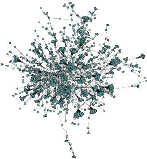
Figure 1: Visualization of the aggregated network of trading contacts, appearing at least $50$ times in the dataset. Here the links are considered as undirected.

In addition to Tab. 1, basic network characteristics are presented in Figs. 3 and 4. Distribution of both the node degrees and the node activity aggregated over the whole period of observation is very broad as shown in Fig. 3.

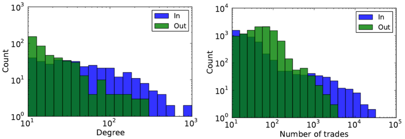
Figure 3: Histogram of node degree (blue: in-degree, green: out-degree) and activity (blue: in-coming activity, green: out-going activity) of the time-aggregated graph.

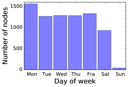
Figure 4: (Average number of links and nodes on different week days.

Figure 4 depicts the average number of nodes and links resolved for each day of the week. Mondays show the highest numbers and other working days a similar level. On Saturdays, the network is less dense and the numbers of nodes and links are the lowest for Sundays.

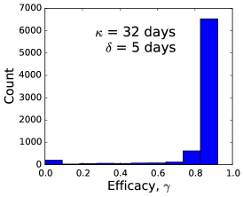
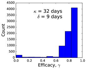
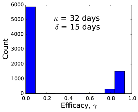
Figure 5: Histogram of the prevalence reduction $\gamma$ for infectious period $\kappa=32$ d and different detection times $\delta$ as indicated in the panels. Each node in the network is chosen as a starting node in a separate simulation with initial infection upon its first appearance in the dataset.

Figure 5 shows the influence of the index nodes and their impact on the success of the control measured in terms of the prevalence reduction $\gamma$ (1)for a fixed infectious period $\kappa=32$ d and different detection times $\delta$. For small $\delta$, we find a prevalence reduction peaked at 90%. As the detection time becomes larger, the control becomes less effective indicated by smaller prevalence reduction. The mean prevalence reduction averaged over all nodes as starting points is presented in Fig 8.

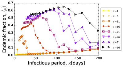
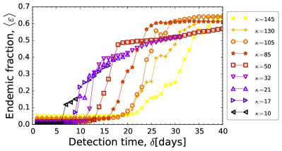
Figure 6: Dependence of the endemic fraction $\varepsilon$: left on the infection period $\kappa$ for different detection times $\delta$ and right on the infectious period $\delta$ for different detection times $\kappa$.

Figs. 6(a) and (b) shows the dependence of the endemic fraction $\varepsilon$ (1) on $\kappa$ (for fixed $\delta$) and on $\delta$ (for fixed $\kappa$) correspondingly.

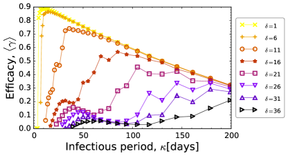
Figure 8: Efficacy or relative prevalence reduction $\gamma$ averaged over all possible index nodes for sustained epidemics in dependence on $\kappa$ (with fixed $\delta$, left panel) and on $\delta$ (with fixed $\kappa$, right panel).

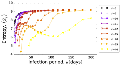
Figure 9: Entropy in dependence on $\kappa$ and $\delta$, which characterizes the heterogeneity in the distribution of efficacy $\gamma$ for different index nodes.

Figure 8 depicts the efficacy or prevalence reduction for sustained epidemics $\gamma$ (2) in dependence on $\kappa$ and $\delta$. This quantity shows how useful the control is, even if we cannot totally stop the disease, which became endemic, and to what extent we could lower the prevalence. There is a fast decrease in the efficacy of the control measures as the detection takes longer.

The efficacy or prevalence reduction $\gamma$ is highly dependent on the index node, and to characterize the heterogeneity we depict in Figure 9 the entropy of the efficacy or prevalence reduction $\gamma$ defined as

$$S_{\gamma}=-\sum_{i}\pi(\gamma_{i})\log[\pi(\gamma_{i})],$$

where the index $i$ enumerates all index nodes, in dependence on $\kappa$ and $\delta$. $\pi(\gamma_{i})$ is the probability for an index node $i$ to have the efficacy $\gamma_{i}$. Entropy in dependence on $\delta$ (Fig. 9, left panel) possesses clearly two flat levels, decreasing from a high to a low one with increasing $\delta$. Thus with early detection, different index nodes lead to very heterogeneous prevalence levels. Later detection leads to epidemics with similar efficacy levels. The dependence of the entropy on the infectious period $\kappa$ (Fig. 9, right panel) exhibits maxima for the intermediate values of $\kappa$. The largest heterogeneity in the efficacy for intermediate infectious periods might be due to the interplay of internal scales of the temporal network.

References

- (1) L. Danon, J. M. Read, T. A. House, M. C. Vernon, and M. Keeling, Proceedings of the Royal Society of London B: Biological Sciences 280, 20131037 (2013).
- (2) A. Barrat, C. Cattuto, A. Tozzi, P. Vanhems, and N. Voirin, Clinical Microbiology and Infection 20, 10 (2014).
- (3) J. Stehlé, N. Voirin, A. Barrat, C. Cattuto, V. Colizza, L. Isella, C. Régis, J. Pinton, N. Khanafer, W. Van den Broeck, and P. Vanhems, BMC medicine 9, 87 (2011).
- (4) C. M. Schneider, V. Belik, T. Couronné, Z. Smoreda, and M. C. González, J. R. Soc. Interface 10, 1742 (2013).
- (5) V. Belik, T. Geisel, and D. Brockmann, Phys. Rev. X 1, 011001 (2011).
- (6) A. Casteigts, P. Flocchini, W. Quattrociocchi, and N. Santoro, International Journal of Parallel, Emergent and Distributed Systems 27, 387 (2012).
- (7) H. Lentz, T. Selhorst, and I. Sokolov, Phys. Rev. Lett. 110, 118701 (2013).
- (8) P. Holme and J. Saramäki, Physics Reports 519, 97 (2012).
- (9) I. Scholtes, N. Wider, R. Pfitzner, A. Garas, C. J. Tessone, and F. Schweitzer, Nat. Commun. 5, 5024 (2014).
- (10) M. Konschake, H. Lentz, F. Conraths, P. Hövel, and T. Selhorst, PLoS ONE 8, e55223 (2013).
- (11) M. Kivelä, R. Pan, K. Kaski, J. Kertész, J. Saramäki, and M. Karsai, J. Stat. Mech. 2012, P03005 (2012).
- (12) P. Bajardi, A. Barrat, L. Savini, and V. Colizza, J. Roy. Soc. Interface 9, 2814 (2012).
- (13) E. Volz and L. A. Meyers, Journal of the Royal Society Interface 6, 233 (2009).
- (14) E. Valdano, L. Ferreri, C. Poletto, and V. Colizza, Phys. Rev. X 5, 021005 (2015).
- (15) C. M. Schneider, A. A. Moreira, J. S. Andrade, S. Havlin, and H. J. Herrmann, Proceedings of the National Academy of Sciences 108, 3838 (2011).
- (16) S. Lee, L. E. Rocha, F. Liljeros, and P. Holme, PLoS ONE 7, e36439 (2012).
- (17) M. Starnini, A. Machens, C. Cattuto, A. Barrat, and R. Pastor-Satorras, J. Theo. Biology 337, 89 (2013).
- (18) K. Büttner, J. Krieter, A. Traulsen, and I. Traulsen, PLoS ONE 8, e74292 (2013).
- (19) S. Liu, N. Perra, M. Karsai, and A. Vespignani, Phys. Rev. Lett. 112, 118702 (2014).
- (20) A. Rizzo, M. Frasca, and M. Porfiri, Phys. Rev. E 90, 042801 (2014).
- (21) J. Tang, C. Mascolo, M. Musolesi, and V. Latora, in World of Wireless, Mobile and Multimedia Networks (WoWMoM), 2011 IEEE International Symposium on a, IEEE (PUBLISHER, ADDRESS, 2011), pp. 1–9.
- (22) M. Pósfai and P. Hövel, New J. Phys. 16, 123055 (2014).
- (23) F. Sélley, A. Besenyei, I. Z. Kiss, and P. L. Simon, arXiv preprint arXiv:1402.2194 (2014).
- (24) T. Gross, C. J. D’Lima, and B. Blasius, Phys. Rev. Lett. 96, 208701 (2006).
- (25) T. Gross and B. Blasius, J. R. Soc. Interface 5, 259 (2008).
- (26) L. Shaw and I. Schwartz, Physical Review E 77, 066101 (2008).
- (27) S. Van Segbroeck and F. C. P. Santos, PLoS Comput Biol 6, e1000895 (2010).
- (28) H. Yang, M. Tang, and T. Gross, Scientific reports 5, (2015).
- (29) R. Brookmeyer, D. F. Stroup, et al., Monitoring the health of populations: statistical principles and methods for public health surveillance. (Oxford University Press, Oxford, 2004).
- (30) L. E. Rocha and V. Blondel, PLoS Comput Biol 9, e1002974 (2013).
- (31) N. Cornick and A. Helgerson, Applied and environmental microbiology 70, 5331 (2004).
- (32) S. M. Fast, M. C. González, J. M. Wilson, and N. Markuzon, Journal of The Royal Society Interface 12, 20141105 (2015).
- (33) V. Grimm, E. Revilla, U. Berger, et al., Science 310, 987 (2005).
- (34) D. Lamouroux, J. Nagler, T. Geisel, and S. Eule, Proceedings of the Royal Society of London B: Biological Sciences 282, 20142805 (2015).
- (35) M. Bigras-Poulin, K. Barfod, S. Mortensen, and M. Greiner, Prev. Vet. Med. 80, 143 (2007).
- (36) L. Audigé, M. Doherr, R. Hauser, and M. Salman, Prev. Vet. Med. 49, 1 (2001).
- (37) A. Ortiz-Pelaez, D. Pfeiffer, R. Soares-Magalhaes, and F. Guitian, Prev. Vet. Med. 76, 40 (2006).
- (38) The HI-Tier database (https://www.hi-tier.de) is administered by the Bavarian State Ministry for Agriculture and Forestry on behalf of the German federal states.
- (39) Directive 2000/15/EC of the European Parliament and the Council of 10 April 2000 amending Council Directive 64/432/EEC on health problems affecting intra-community trade in bovine animals and swine.