Relaxation Methods for Hyperbolic PDE Mixed-Integer Optimal Control Problems

Abstract.

We extend the convergence analysis for methods solving PDE-constrained optimal control problems containing both discrete and continuous control decisions based on relaxation and rounding strategies to the class of first order semilinear hyperbolic systems in one space dimension. The results are obtained by novel a-priori estimates for the size of the relaxation gap based on the characteristic flow, fixed-point arguments and particular regularity theory for such mixed-integer control problems. As an application we consider a relaxation model for optimal flux switching control in conservation laws motivated by traffic flow problems.

1. Introduction

Decision taking, e. g., specifying on/off for some fixed actuator on a plant, is a very elementary control mechanism. Critical infrastructure systems such as gas pipeline networks, water canal networks or highway traffic networks are for instance controlled by switching valves [23], weirs [20] or speed limit signs [15], respectively. These decision are possibly to be taken in combination with determining additional continuously variable parameters such as the outlet pressure of a compressor in the gas network example. Further modeling aspects of such problems are discussed in [13]. We will refer to the open-loop optimization of such heterogeneous controls as a mixed-integer optimal control problem. In the literature, such problems are also called discrete-continuous, hybrid or switching optimal control problems.

A method for solving such problems numerically should yield integer feasible solutions based on sufficiently accurate approximations of the plant’s dynamics. Due to the combinatorial complexity this is a difficult problem in general. In particular, it becomes a real challenge when the plant is modeled using partial differential equations (PDEs) as it is expedient for example in the mentioned infrastructure systems in nonstationary scenarios on large scale networks. Thus, several different solution approaches have already been proposed in the literature. They can be classified as total-discretization-, reformulation- and direct relaxation-based and each of them have there assets and drawbacks.

Total discretization of the underlying dynamical system obviously leads to mixed-integer nonlinear programs (MINLPs). These become typically large, in particular in the PDE case. Hence, solving such MINLPs requires structure exploiting algorithms. If they are available, such methods can provide global optimal solutions. This approach is followed for example in [9] for gas networks or in [11] for traffic flow.

Reformulations turn the mixed-integer optimal control problem into—on some level—equivalent formulations which can then be solved with existing numerical methods. For example, a variable time transformation method yields a continuous formulation [21, 10]. This approach is yet limited to problems governed by ordinary differential equations (ODEs). Optimal switching controls can in some cases be sophisticatedly characterized using the viscosity solution of a Hamilton-Jacobi-Bellman system, see [7] for ODE problems and [26] for a generalization to PDEs. However, in particular in the PDE case, the Hamilton-Jacobi-Bellman system is again typically large and numerically a difficult problem. Complementarity-based reformulations are used in [3] and have been applied to gas network optimization in [4]. The resulting system then require special nonlinear solvers, or additional relaxation techniques.

Direct relaxation of the decision variables obviously turns the problem into a fully continuous setting. The resulting problem can then be solved with well-established nonlinear optimal control techniques and integer solutions can be recovered from rounding. For ODE problems, it has been shown that the relaxation gap, i. e., the distance of the optimal value for the relaxed problem and the one corresponding to the rounded solution, can be made arbitrary small using relaxation for a convexified problem together with a constructive rounding strategy [24]. The so obtained epsilon-optimal controls may involve frequent switching, but suboptimal solutions can still be obtained including combinatorial constraints limiting for example the number of switches [25]. The approach has also been generalized to dealing with vanishing constraints [18] and to mixed-integer control problems for abstract semilinear evolutions on Banach spaces using semigroup theory [14]. The generalization to Banach spaces covers semilinear PDE cases, but the analysis in [14] assumes a certain degree of smoothness of the solution. Due to the inherent discontinuities of the integer control interfering with the solution, these regularity assumptions are only known to be valid in parabolic cases due to the natural smoothing properties of ellipic operators (examples are discussed [14]). In particular, these regularity assumptions are known to fail for classical solutions and are in general very difficult to be verified for weak solutions in hyperbolic cases. Unfortunately, all examples mentioned at the beginning naturally involve hyperbolic PDEs which are at present not supported by the available theory for this approach.

The main contribution of this paper is to extend the analysis for the direct relaxation approach to semilinear hyperbolic PDEs with distributed mixed-integer control. Instead of employing semigroup theory on classical Sobolev spaces as in [14], we obtain novel a-priori estimates on the size of the relaxation gap using the method of characteristics and particular regularity results on semi-classical Sobolev spaces. This is an important step to establish relaxation techniques for optimization of the mentioned infrastructure systems. For instance, transient gas network operation can often be accurately modeled using semilinear Euler-equations [1]. For an application of the results obtained in this paper to gas-network optimization, valve switching is then to be modeled as a distributed control on very small pipe sections. This is intended as future work. In this paper, we will discuss the application of the method to a relaxation model of nonlinear conservation laws motivated by traffic flow control.

The paper is organized as follows. In Section 2 we give a detailed problem formulation for a semilinear hyperbolic mixed-integer optimal control problem and relate it to a relaxed and convexified problem. In Section 3 we estimate the gap made by this approach in terms of the integrated difference of two controls. The latter quantity is not a norm on the respective control spaces which make the estimates technically difficult. The estimates yield a convergence result for the relaxation method in Proposition 8. In Section 4, we employ the relaxation approach to the already mentioned example motivated by traffic flow, where we use an adjoint-equation based gradient-decent algorithm to compute solutions to a relaxed problem and we apply rounding strategies in order to verify the predicted convergence numerically. In Section 5, we draw a brief conclusion.

2. Problem Formulation and the Relaxation Approach

For some real constants $L,T>0$, a natural number $n$, a diagonal matrix function $\Lambda=\text{diag}(\lambda_{1},\ldots,\lambda_{n})$ with $\lambda_{i}\mathcal{\colon}[0,L]\to\mathbb{R}$, $i\in\{1,\ldots,n\}$, normed vector spaces $U$ and $V$ and a nonlinear function $f\mathcal{\colon}\mathbb{R}^{n}\times U\times V\to\mathbb{R}^{n}$, we consider a controlled system of semilinear hyperbolic PDEs in two variables $t$ (time) and $x$ (a single space variable)

$$y_{t}+\Lambda(x)y_{x}=f(y,u(t),v(t))\quad\text{on}~{}(0,T)\times(0,L)$$ (1)

for an unkown vector function $y=(y_{1},\ldots,y_{n})^{\top}\mathcal{\colon}(0,T)\times(0,L)\to\mathbb{R}^{n}$ and two controls $u\mathcal{\colon}[0,T]\to U$ and $v\mathcal{\colon}[0,T]\to V$. We assume that, for some $r\in\{1,\ldots,n\}$, $\lambda_{i}<0$ for $i\in\{1,\ldots,r\}$ and $\lambda_{i}>0$ for $i=\{r+1,\ldots,n\}$ and set $y^{-}=(y_{1},\ldots,y_{r})^{\top}$, $y^{+}=(y_{r+1},\ldots,y_{n})^{\top}$, so that $y=(y^{-},y^{+})^{\top}$. Further, we consider (1) subject to boundary conditions

$$\begin{pmatrix}y^{-}(t,L)\\ y^{+}(t,0)\end{pmatrix}=\begin{pmatrix}G_{--}&G_{-+}\\ G_{+-}&G_{++}\end{pmatrix}\begin{pmatrix}y^{-}(t,0)\\ y^{+}(t,L)\end{pmatrix}+\begin{pmatrix}d^{-}(t)\\ d^{+}(t)\end{pmatrix},\quad\text{on}~{}(0,T)$$ (2)

and an initial condition

$$y(0,x)=\bar{y}(x)\quad\text{on}~{}[0,L],$$ (3)

where we assume that $G_{--}\in\mathbb{R}^{r\times r}$, $G_{-+}\in\mathbb{R}^{r\times(n-r)}$, $G_{+-}\in\mathbb{R}^{(n-r)\times r}$, $G_{++}\in\mathbb{R}^{(n-r)\times(n-r)}$, $d^{-}\mathcal{\colon}[0,T]\to\mathbb{R}^{r}$, $d^{+}\mathcal{\colon}[0,T]\to\mathbb{R}^{(n-r)}$, and $\bar{y}\mathcal{\colon}[0,L]\to\mathbb{R}^{n}$. The diagonal form in (1) is without loss of generality, because it can be achieved by a change of variables for many physical systems, see e. g., [8, 6].

Our interest will be to find controls $u$ and $v$ (piecewise smooth and piecewise constant, respectively) that minimize a cost criterion

$$J(y(T,\cdot))=\int_{0}^{L}g(y(T,x))\,dx,$$ (4)

where $g\mathcal{\colon}\mathbb{R}^{n}\to\mathbb{R}$ is a non-linear function, subject to the ordinary control constraint that

$$u(t)\in\mathcal{U}$$ (5)

for some closed (and otherwise arbitrary) set $\mathcal{U}\subset U$ and the discrete control constraint

$$v(t)\in\{v^{1},v^{2},\ldots,v^{M}\}$$ (6)

for some given values $v^{1},v^{2},\ldots,v^{M}\in V$, $M\in\mathbb{N}$.

To this end, we note that for any piecewise smooth $u$ and any piecewise constant $v$, the equation (1) is equivalent to

$$y_{t}+\Lambda y_{x}=\sum_{j=1}^{M}\alpha_{j}f(y,u,v^{j})\quad\text{on}~{}(0,T)\times(0,L)$$ (7)

with new controls $\alpha_{j}=\alpha_{j}(t)\in\{0,1\}$, $j=1,\ldots,M$, satisfying $\sum_{j=1}^{M}\alpha_{j}(t)=1$ for almost every $t$. We will in the following estimate the gap (measured in terms of the norm of $y$) of weak solutions for (7) (hence solutions to the original problem) and the relaxed problem

$$y_{t}+\Lambda y_{x}=\sum_{j=1}^{M}\beta_{j}f(y,u,v^{j})\quad\text{on}~{}(0,T)\times(0,L)$$ (8)

with controls $\beta_{j}=\beta_{j}(t)\in[0,1]$, $j=1,\ldots,M$, satisfying $\sum_{j=1}^{M}\beta_{j}(t)=1$ for almost every $t$. Note that we only replaced the condition “new controls in $\{0,1\}$” with the condition “new controls in $[0,1]$”. Further, observe that the minimization of (4) subject to the relaxed problem (8) with the boundary data (2) and (3) and control constraints

$$\eqref{eq:Cconstraint},\quad\beta_{j}(t)\in[0,1],~{}j=1,\ldots,M\quad\text{and}\quad\sum_{j=1}^{M}\beta_{j}(t)=1,\quad t\in(0,T)~{}\text{a.\,e.}$$ (9)

is an optimal control problem of a semilinear hyperbolic system in standard form which can be solved efficiently with existing numerical methods [16, 2].

The main motivation for the a-priori estimates derived in Section 3 is the following observation proved in [24].

Lemma 1.

Let $\beta\mathcal{\colon}[0,T]\to[0,1]^{M}$ be a measurable function such that $\sum_{j=1}^{M}\beta_{j}(t)=1$ for almost every $t$. Then, there exists a piecewise constant function $\alpha\mathcal{\colon}[0,T]\to\{0,1\}^{M}$ satisfying $\sum_{j=1}^{M}\alpha_{j}(t)=1$ for all $t\in[0,T]$ such that

$$\max_{j=1,\ldots,M}\sup_{t\in[0,T]}\left|\int_{0}^{t}\beta_{j}(s)-\alpha_{j}(s)\,ds\right|\leq(M-1)\Delta t.$$ (10)

where $\Delta t$ is the length of the largest subinterval where $\alpha$ is taken constant.

Remark 2.

The proof in [24] for the existence of $\alpha$ as in the previous Lemma is constructive, giving rise to a numerical method that was also explicitly used in [14]. Moreover, it has recently been show that the right hand side in (10) can been improved to $\mathcal{O}(\log(M))\Delta t$ [19].

We are therefore interested in estimates on the relaxation gap in terms of the left hand side of (10). Note that this quantity is not a norm and that these estimates therefore are neither classical nor obvious. For our analysis, we will consider solutions of (1) or (8), respectively, subject to the boundary conditions (2) and the initial condition (3) in the sense of the forward characteristic flow. Letting $\Omega_{T}=[0,T]\times[0,L]$ and $s_{i}(t;\tau,\sigma)$, $i\in\{1,\ldots,n\}$ denote the characteristic curves defined by

$$\frac{d}{dt}s_{i}=\lambda_{i}(s_{i}),\quad s_{i}(\tau;\tau,\sigma)=(\tau,\sigma),\quad(\tau,\sigma)\in\Omega_{T}$$ (11)

the forward characteristic flow of (8) is obtained as a fixed point $y\mathcal{\colon}\Omega_{T}\to\mathbb{R}^{n}$ of the following integral transformation

$$\psi(y)(\tau,\sigma)=(\psi_{1}(y)(\tau,\sigma),\ldots,\psi_{n}(y)(\tau,\sigma))$$ (12)

with $\psi_{i}(y)(\tau,\sigma)$ defined recursively as

$$\psi_{i}(y)(\tau,\sigma)=Y_{i}(\psi;\tau,\sigma)+\sum_{j=1}^{M}\int_{t_{i}^{*}}^{\tau}\beta_{j}(t)f(y(t,s_{i}(t;\tau,\sigma)),u(t),v^{j})\,dt,$$ (13)

where $t_{i}^{*}=t_{i}^{*}(\tau,\sigma)$ denotes the intersection time of the curve $s_{i}(\cdot;\tau,\sigma)$ with the boundary of $\Omega_{T}$ backward in time and $Y_{i}(\psi;\tau,\sigma)$ is defined as the $i$-th component of

$$\begin{cases}\begin{pmatrix}G_{--}&G_{-+}\\ G_{+-}&G_{++}\end{pmatrix}\begin{pmatrix}\psi^{-}(y)(t_{i}^{*},0)\\ \psi^{+}(y)(t_{i}^{*},L)\end{pmatrix}+\begin{pmatrix}d^{-}(t_{i}^{*})\\ d^{+}(t_{i}^{*})\end{pmatrix}\quad&\text{if $t_{i}^{*}>0$},\\ \bar{y}(t_{i}^{*},s_{i}(t_{i}^{*};\tau,\sigma))\quad&\text{if $t_{i}^{*}=0$},\end{cases}$$ (14)

where $\psi^{-}=(\psi_{1},\ldots,\psi_{r})^{\top}$ and $\psi^{+}=(\psi_{r+1},\ldots,\psi_{n})^{\top}$. The so defined solution coincides with the usual weak solution of (1) or (8), respectively, subject to the boundary conditions (2) and the initial condition (3) in appropriate spaces [12].

3. A-priori Estimates on the Relaxation Gap

The subsequent analysis is based on a particular regularity result for hyperbolic initial boundary value problems obtained in [22], giving a sufficient condition for the solution defined by the forward characteristic flow having bounded distributional derivatives along almost every characteristic curve if the initial and boundary data is piecewise smooth. To be more specific, for any $p,q,\mu\in\mathbb{N}$ and any family of disjoint open sets $\Omega_{m}\subset\mathbb{R}^{p}$, $m=1,\ldots,\mu$, we will denote by

$$\bigotimes_{m=1}^{\mu}W^{1,1}(\Omega_{m};\mathbb{R}^{q}),\qquad\bigotimes_{m=1}^{\mu}C^{0}(\Omega_{m};\mathbb{R}^{q})$$ (15)

the set of functions $h$ defined on the closure of $\bigcup_{m=1}^{\mu}\Omega_{m}$ with image in $\mathbb{R}^{q}$ so that their restriction to $\Omega_{m}$ belongs to the classical Sobolev space $W^{1,1}(\Omega_{m};\mathbb{R}^{q})$ or the Banach space $C^{0}(\Omega_{m};\mathbb{R}^{q})$, respectively.

Then, we make the following assumptions.

Hypothesis 3.

The components of $\Lambda$, $\lambda_{i}:[0,L]\to\mathbb{R}$, $i\in\{1,\ldots,n\}$ are Lipschitz-continuous. The functions $y\to f(y,u,v^{j})$ are smooth and satisfy $f(0,u,v^{j})=0$ for all $j=1,\ldots,M$ and $u\in U$. The function $u\to f(y,u,v^{j})$ is locally Lipschitz-continuous on $U$ for all $j=1,\ldots,M$ and $y\in Y$. Further, for all $T>0$, there exist finitely many points $0=\tau_{0}<\tau_{1}<\ldots<\tau_{K-1}<\tau_{K}=T$ and $0=x_{0}<x_{1}<\ldots<x_{\nu-1}<x_{\nu}=L$ so that the initial and boundary data satisfies $\bar{y}\in\bigotimes_{i=1}^{\nu}W^{1,1}(x_{i},x_{i+1};\mathbb{R}^{n})$, $d^{-}\in\bigotimes_{i=1}^{K}W^{1,1}(\tau_{i},\tau_{i+1};\mathbb{R}^{r})$, and $d^{+}\in\bigotimes_{i=1}^{K}W^{1,1}(\tau_{i},\tau_{i+1};\mathbb{R}^{(n-r)})$.

These assumptions yield the following wellposedness result.

Lemma 4.

Under Hypothesis 3 and for any piecewise smooth control $u\mathcal{\colon}[0,\infty)\to U$ there exist constants $T,K>0$ such that (8) subject to the boundary conditions (2) and the initial condition (3) admits a unique solution $y$ in $C([0,T];L^{\infty}(0,L;\mathbb{R}^{n})\cap L^{1}(0,L;\mathbb{R}^{n}))$ for all piecewise smooth controls $\beta\mathcal{\colon}[0,T]\to[0,1]^{M}$. In particular, this solution is given as the (unique) fixed point of (12)–(14) resulting from a strict contraction with contraction constant $\frac{1}{2}$ on $\mathcal{Y}=C([0,T];L^{1}(0,L;\mathbb{R}^{n}))$ equipped with the norm

$$\|y\|_{\dagger}=\sup_{t\in[0,T]}e^{-Kt}\sum_{i=1}^{n}\int_{0}^{L}|y_{i}(t,x)|dx.$$ (16)

Proof.

Hypothesis 3 implies that the initial and boundary data, respectively, satisfies $\bar{y}\in L^{p}(0,L;\mathbb{R}^{n})$, $d^{-}\in L^{p}(0,T;\mathbb{R}^{r})$ and $d^{+}\in L^{p}(0,T;\mathbb{R}^{(n-r)})$ for all $p\in\{1,\infty\}$ and all $T>0$ and that $f$ is locally Lipschitz-continuous in $y$. Noting that all feasible $\beta$ are uniformly bounded by one in the sup-norm, the result follows from classical fixed-point arguments [8], [6]. ∎

In order to obtain further regularity properties of the solution, we adapt the following definitions from [22]. For any piecewise smooth control $\beta\mathcal{\colon}[0,\infty)\to[0,1]^{M}$ with discontinuities at $\{\theta_{i}\}_{i=1}^{\infty}$, let $E^{0}(\beta)$ denote the union of all forward characteristic curves $s_{i}$ generated by $\Lambda$ (and their reflections at the boundaries) which lie in $\Omega_{\infty}=[0,\infty)\times[0,L]$, which emerge from the boundary points

$$\{(0,x_{0}),\ldots,(0,x_{\nu}),~{}(\tau_{0},0),\ldots,(\tau_{K},0),~{}(\tau_{0},L),\ldots,(\tau_{K},0)\}$$ (17)

and their intersection points with the sets $\{\theta_{i}\}\times[0,L]$ for all $i=1,\ldots,\infty$. Further, for $k\in\mathbb{N}$, let $E^{k}(\beta)$ be the union of $E^{k-1}(\beta)$ and all forward characteristic curves (and their boundary reflections) emerging from intersection points of characteristics that defined $E^{k-1}$. Let $E_{T}(\beta)$ be the closure of all points in $\bigcup_{k=1}^{\infty}E^{k}(\beta)\cap\Omega_{T}$. Supposing that

$$E_{T}(\beta)\cap\{t\}\times[0,L]~{}\text{is nowhere dense in}~{}\{t\}\times[0,L],\quad t\in(0,T],$$ (18)

$E_{T}(\beta)$ is defined by finitely many discrete curves, which divide $\Omega_{T}$ up into finitely many simply connected open sets $\Omega_{T}^{m}$, $m=1,\ldots,\mu$, $\mu\in\mathbb{N}$. We set

$$W^{1,1}_{*}(\Omega_{T}\setminus E_{T}(\beta)):=\bigotimes_{m=1}^{\mu}W^{1,1}(\Omega_{T}^{m}),\quad C^{0}_{*}(\Omega_{T}\setminus E_{T}(\beta)):=\bigotimes_{m=1}^{\mu}C^{0}(\Omega_{T}^{m}).$$ (19)

With this notation, we note the following additional regularity of the $L^{1}$-solution for piecewise smooth data and controls.

Lemma 5.

Under Hypothesis 3 and for any piecewise smooth control $u\mathcal{\colon}[0,\infty)\to U$ and any piecewise smooth control $\beta\mathcal{\colon}[0,\infty)\to[0,1]^{M}$, there exist a constant $T>0$ (less or equal to the constant obtained in Lemma 4) such that (18) holds for the set $E_{T}(\beta)$ defined above. Moreover, it holds that the solution $y$ of (8) subject to the boundary conditions (2) and the initial condition (3) obtained in Lemma 4 satisfies

$$y\in W^{1,1}_{*}(\Omega_{T}\setminus E_{T}(\beta))\cap C^{0}_{*}(\Omega_{T}\setminus E_{T}(\beta)).$$ (20)

Proof.

The result follows directly from [22, Theorem 3.1 and Remark 3.3] applied iteratively on time intervals where $d^{-}$, $d^{+}$, $u$ and $\beta$ are jointly continuous. ∎

Moreover, we will need the following fixed point argument.

Lemma 6.

Consider a Banach space $(X,\|\cdot\|_{X})$. Let $\mathcal{X}:=\{x\in X:\|x\|_{\dagger}<\infty\}$ for some norm $\|\cdot\|_{\dagger}$ satisfying

$$\underline{c}\|x\|_{X}\leq\|x\|_{\dagger}\leq\bar{c}\|x\|_{X},\quad x\in X.$$ (21)

Let $\phi,\psi\mathcal{\colon}\mathcal{X}\to\mathcal{X}$ be continuous mappings such that

$$\|\phi(x)-\phi(\zeta)\|_{\dagger}\leq\frac{1}{2}\|x-\zeta\|_{\dagger},\quad\|\psi(x)-\psi(\zeta)\|_{\dagger}\leq\frac{1}{2}\|x-\zeta\|_{\dagger},\quad x,\zeta\in\mathcal{X}.$$ (22)

Suppose that there exists a constant $C>0$ so that

$$\|\phi(x^{*})-\psi(x^{*})\|_{X}\leq C,$$ (23)

where $x^{*}\in\mathcal{X}$ denotes the (unique) fixed-point of $\phi$ in $X$. For the (unique) fixed point $\zeta^{*}\in\mathcal{X}$ of $\psi$ in $X$ it then holds

$$\|x^{*}-\zeta^{*}\|_{X}\leq 2\underline{c}^{-1}\bar{c}C.$$ (24)

Proof.

By the triangular inequality and (21) we have

$$\|x^{*}-\zeta^{*}\|_{\dagger}\leq\bar{c}\|\phi(x^{*})-\psi(x^{*})\|_{X}+\|\psi(x^{*})-\psi(\zeta^{*})\|_{\dagger}.$$ (25)

Using (22) and (23), this yields

$$\|x^{*}-\zeta^{*}\|_{\dagger}\leq\bar{c}C+\frac{1}{2}\|x^{*}-\zeta^{*}\|_{\dagger},$$ (26)

and equivalently (24) using again (21). ∎

With the above auxilary results, we can now prove the following a-priori estimate on the difference of two solutions corresponding to two different controls with a bounded integerated difference.

Theorem 7.

Assume Hypothesis 3 and let $u\mathcal{\colon}[0,\infty)\to U$, $\beta\mathcal{\colon}[0,\infty)\to[0,1]^{M}$ and $\tilde{\beta}\mathcal{\colon}[0,\infty)\to[0,1]^{M}$ be piecewise smooth controls. Moreover, assume that for some given $\varepsilon>0$ and $T$ sufficiently small,

$$\max_{j=1,\ldots,M}\sup_{t\in[0,T]}\left|\int_{0}^{t}\beta_{j}(s)-\tilde{\beta}_{j}(s)\,ds\right|\leq\varepsilon.$$ (27)

Then, there exists a constant $\bar{C}=\bar{C}(u,\beta)>0$ (independent of $\tilde{\beta}$) so that

$$\|y(u,\beta)-y(u,\tilde{\beta})\|_{Y}\leq\bar{C}\varepsilon,$$ (28)

where $y(u,\beta)$ and $y(u,\tilde{\beta})$ denote the $L^{1}$-solutions of the relaxed problem (8) subject to the boundary conditions (2), initial condition (3) and the control constraints (9) with controls $(u,\beta)$ and $(u,\tilde{\beta})$, respectively.

Proof.

Let $T$ be less or equal to the constant $T$ obtained in Lemma 5 for the fixed control $(u,\beta)$. Moreover, let $\psi$ denote the integral transformation (12)–(14) associated to the fixed control $(u,\beta)$ and let $\phi$ denote the corresponding integral transformation associated to the fixed control $(u,\tilde{\beta})$. By Lemma 4, there exists $K>0$ such that both transformations are strict contractions with contraction constant $\frac{1}{2}$ on $(\mathcal{Y})$ with respect to the norm $\|\cdot\|_{\dagger}$ defined in (16), possessing the unique fixed points $y=y(u,\beta)$ and $\tilde{y}=y(u,\tilde{\beta})$, respectively.

We will now show existence of a constant $\tilde{C}$ such that

$$\int_{0}^{L}|\psi_{i}(y)(\tau,\sigma)-\phi_{i}(y)(\tau,\sigma)|d\sigma\leq\tilde{C}\varepsilon,~{}i=1,\ldots,n,~{}t\in[0,T]$$ (29)

holds for the fixed point $y=y(u,\beta)$.

We have for $\tau\in[0,T]$ and $0\leq t^{*}_{i}=t^{*}_{i}(\tau,\sigma)<\tau$

$$\int_{0}^{L}\left|\psi_{i}(y)(\tau,\sigma)-\phi_{i}(y)(\tau,\sigma)\right|d\sigma\leq\|Y_{i}(\psi;\tau,\sigma)-Y_{i}(\phi;\tau,\sigma)\|~{}+$$ (30)

$$\qquad\sum_{j=1}^{M}\int_{0}^{L}\left|\int_{t_{i}^{*}}^{\tau}[\beta_{j}(\vartheta)-\tilde{\beta}_{j}(\vartheta)]f(y(\vartheta,s_{i}(\vartheta;\tau,\sigma)),u(\vartheta),v^{i})\,d\vartheta\right|d\sigma.$$

Integration by parts for the integral in $\vartheta$ yields

$$\sum_{j=1}^{M}\int_{0}^{L}\left|\int_{t_{i}^{*}}^{\tau}[\beta_{j}(\vartheta)-\tilde{\beta}_{j}(\vartheta)]f(y(\vartheta,s_{i}(\vartheta;\tau,\sigma)),u(\vartheta),v^{j})\,d\vartheta\right|d\sigma\leq$$ (31)

$$\quad\sum_{j=1}^{M}\int_{0}^{L}\int_{t_{i}^{*}}^{\tau}\left|\int_{0}^{\vartheta}\beta_{j}(\xi)-\tilde{\beta}_{j}(\xi)\,d\xi\right|\left|D_{\vartheta}f(y(\vartheta,s_{i}(\vartheta;\tau,\sigma)),u(\vartheta),v^{j})\right|d\vartheta d\sigma~{}+$$

$$\quad\sum_{j=1}^{M}\int_{0}^{L}\left|\int_{0}^{\tau}\beta_{j}(\xi)-\tilde{\beta}_{j}(\xi)\,d\xi\right||f(y(\tau,s_{i}(\tau;\tau,\sigma)),u(\tau),v^{j})|d\sigma~{}+$$

$$\quad\sum_{j=1}^{M}\int_{0}^{L}\left|\int_{0}^{t_{i}^{*}}\beta_{j}(\xi)-\tilde{\beta}_{j}(\xi)\,d\xi\right||f(y(t_{i}^{*},s_{i}(t_{i}^{*};\tau,\sigma)),u(t_{i}^{*}),v^{j})|d\sigma.$$

By assumption (27), this estimate becomes

$$\sum_{j=1}^{M}\int_{0}^{L}\left|\int_{t_{i}^{*}}^{\tau}[\beta_{j}(\vartheta)-\tilde{\beta}_{j}(\vartheta)]f(y(\vartheta,s_{i}(\vartheta;\tau,\sigma)),u(\vartheta),v^{j})\,d\vartheta\right|d\sigma\leq$$ (32)

$$\quad\varepsilon\sum_{j=1}^{M}\bigg{(}\int_{t_{i}^{*}}^{\tau}\int_{0}^{L}\left|D_{\vartheta}f(y(\vartheta,s_{i}(\vartheta;\tau,\sigma)),u(\vartheta),v^{j})\right|d\sigma~{}+$$

$$\quad\int_{0}^{L}|f(y(\tau,s_{i}(\tau;\tau,\sigma)),u(\tau),v^{j})|+|f(y(t_{i}^{*},s_{i}(t_{i}^{*};\tau,\sigma)),u(t_{i}^{*}),v^{j})|d\sigma\bigg{)}.$$

The chain rule yields

$$\int_{0}^{L}\left|D_{\vartheta}f(y(\vartheta,s_{i}(\vartheta;\tau,\sigma)),u(\vartheta),v^{j})\right|d\sigma\leq$$ (33)

$$\qquad\sum_{k=1}^{n}\int_{0}^{L}\bigg{|}D_{y_{k}}f(y(\vartheta,s_{i}(\vartheta;\tau,\sigma)),u(\vartheta),v^{j})\bigg{|}\bigg{|}D_{\vartheta}y_{k}(\vartheta,s_{i}(\vartheta;\tau,\sigma))\bigg{|}~{}+$$

$$\qquad\bigg{|}D_{u}f(y(\vartheta,s_{i}(\vartheta;\tau,\sigma)),u(\vartheta),v^{j})\bigg{|}\bigg{|}D_{\vartheta}u(\vartheta)\bigg{|}d\sigma.$$

The assumptions in Hypothesis 3 on $f$, the assumed regularity of $u$ and the regularity result on $y=y(u,\beta)$ in Theorem 5 now yields that all terms in absolute values appearing in the right hand side of (33) are essentially bounded. Since all remaining terms in the right hand side of (32) are finite and independent of $\tilde{\beta}$, there exists a constant $\hat{C}$ independent of $\tilde{\beta}$ such that

$$\sum_{j=1}^{M}\int_{0}^{L}\left|\int_{t_{i}^{*}}^{\tau}[\beta_{j}(\vartheta)-\tilde{\beta}_{j}(\vartheta)]f(y(\vartheta,s_{i}(\vartheta;\tau,\sigma)),u(\vartheta),v^{j})\,d\vartheta\right|d\sigma\leq\hat{C}\varepsilon.$$ (34)

Moreover, for $\|Y_{i}(\psi;\tau,\sigma)-Y_{i}(\phi;\tau,\sigma)\|$, we can use (14). For $i\in\{1,\ldots,r\}$ and $(\tau,\sigma)$ such that $t_{i}^{*}>0$ for all $\sigma\in[0,L]$, we obtain

$$\|Y_{i}(\psi;\tau,\sigma)-Y_{i}(\phi;\tau,\sigma)\|\leq\|G\|\left\|\begin{pmatrix}\psi^{-}(y)(t_{i}^{*},0)-\phi^{-}(y)(t_{i}^{*},0)\\ \psi^{+}(y)(t_{i}^{*},0)-\phi^{+}(y)(t_{i}^{*},0)\end{pmatrix}\right\|$$ (35)

and a similar estimate is obtained in the other cases. We can then repeat the above estimates for each of the components of the vectors in the right hand side of (35). Since $t_{i}^{*}<\tau$ and since the estimate becomes trivial for $t_{i}^{*}=0$, the existence of a constant $\tilde{C}$ independent of $\tilde{\beta}$ such that (29) follows from induction.

Finally, we note that $X=C([0,T];L^{1}(0,L;\mathbb{R}^{n}))$ is a Banach space for which (21) holds with $\underline{c}=e^{-KT}$ and $\bar{c}=1$. So the desired estimate (28) follows (29) and Lemma 6 with $\mathcal{X}=\mathcal{Y}$ and $\bar{C}=2\underline{c}^{-1}\bar{c}n\tilde{C}=2e^{KT}n\tilde{C}$. ∎

A combination of Theorem 7 and Lemma 1 yields a method for solving the mixed-integer optimal control problem stated in Section 2 subject to Hypothesis 3 up to any requested accuracy. We state this method in form of the following proposition and remarks.

Proposition 8.

Assume Hypothesis 3 and suppose that for some sufficiently small $T$ the minimization of (4) subject to the relaxed problem (8) with the boundary data (2) and (3) and control constraints (9) admits a piecewise smooth optimal control $(u,\beta)$ with associate optimal value $J^{*}$. Let $\alpha^{k}$ be a sequence of controls $\alpha^{k}\mathcal{\colon}[0,T]\to\{0,1\}$ given by Lemma 1 obtained from $\beta$ for a sequence $\Delta t^{k}\to 0$ as $k\to\infty$. Define $v^{k}\mathcal{\colon}[0,T]\to V$ by $v^{k}(t)=\sum_{i=1}^{M}\alpha^{k}(t)v^{k}$. Then $y(u,v^{k})$ converges strongly to $y(u,\beta)$ as $k\to\infty$. In particular, for norm-continuous cost functions $J$,

$$\lim_{k\to\infty}J(y(u,v^{k}))=J^{*}.$$ (36)

For Lipschitz-continuous $J$, the convergence speed is at least linear in $\Delta t^{k}$.

Proof.

This follows from applying Lemma 1 with $\alpha=\alpha^{k}$ and Theorem 7 with $\tilde{\beta}=\alpha^{k}$ and $\varepsilon=(M-1)\Delta t^{k}$ for each fixed $k$. ∎

Remark 9.

We may relax the assumption of existence of a piecewise smooth optimal control $(u,\beta)$ in Proposition 8 by existence of a piecewise smooth suboptimal control $(u,\beta)$ with $J^{*}=J(y(u,\beta))$. The statement of the Proposition then does not change otherwise, but it clearly yields a slightly weaker conclusion. We may also include combinatorial constraints on the integer controls, e. g., bounding the number of switches between the modes. Then, we do in general not obtain the convergence (36), but the relaxation method then still yields asymptotically a monotonic decreasing sequence $J(y(u,v^{k}))$ of suboptimal solutions as $k\to\infty$. Moreover, the relaxation method can also deal with state constraints. Details of these extensions are discussed in [14].

Remark 10.

Note that Theorem 7, Proposition 8 and Remark 9 are stated for sufficiently small $T>0$ guaranteeing the existence of the solution for the control $(u,\beta)$ both in the sense of Lemma 4 and Lemma 5. However, this limitation can be removed under additional assumptions on $f$, $\Lambda$ and the system’s dimension. For example, is well-known that if the mappings $y\mapsto f(y,u,v^{j})$ and $x\mapsto\Lambda(x)$ are Lipschitz-continuous, then the $L^{1}$-solution (coinciding with the $L^{\infty}$-solution) in the sense of Lemma 4 exists for all $T>0$. Further, in the important case of $n=2$, we have $E_{T}(\beta)=E^{0}_{T}(\beta)$ and hence $E_{T}(\beta)$ satisfies (18) for all $T>0$. In that cases, for example, Theorem 7 and Proposition 8 hold for arbitrary $T$. Nevertheless, for $n\geq 3$, even if the $L^{1}$-solution exists and coincides with the $L^{\infty}$-solution globally in time, $E_{T}(\beta)$ may violate (18). For $n=3$, an example is also given in [22]. Hence, in general, for $n\geq 3$, (18) must be explicitly checked.

4. Application to flux switching control of conservation laws

We consider the integer controlled semilinear hyperbolic system

$$\eta_{t}+\xi_{x} =0,$$ (37)

$$\xi_{t}+a^{2}\eta_{x} =-\kappa^{-1}(\xi-g(\eta,v)),\quad v\in\{1,2\}$$

with $g(\eta,1)=\frac{1}{2}\eta^{2}$, $g(\eta,2)=-\frac{1}{2}\eta^{2}$, $\kappa>0$ and $a^{2}$ such that $a^{2}-\eta^{2}\geq 0$. In characteristic variables $y_{1}=\eta+a\xi$ and $y_{2}=\eta-a\xi$, the system (37) can be written as (1) with $\Lambda=\text{diag}(a,-a)$ and a nonlinear function $f(y,u,v)$ independent of $u$.

For sufficiently small $\kappa$, the system (37) is an approximation of the control system

$$\eta_{t}\pm{\textstyle\frac{1}{2}}\eta^{2}_{x}=0$$ (38)

where the control just consists of switching the sign in the flux function of the conservation law (38). The approximation holds in the sense that, for fixed $v$, up to second order in $\kappa$

$$\eta_{t}\pm{\textstyle\frac{1}{2}}\eta^{2}_{x}=\kappa((a^{2}-\eta^{2})\eta_{x})_{x},$$ (39)

see, [17, 5]. Such flux switching control problems appear for example when traffic flow modeled by conservation laws is supposed to be optimized by switching dynamic speed limit signs as in [15]. Since Burger’s equation is a typical test problem for traffic flow, this example shall demonstrate that the relaxation method investigated in this paper is a very efficient way to solve such problems with the advantage of being supported by a convergence theory and being applicable up to the same discretization levels that can be handled by optimal control techniques for hyperbolic systems without integer confinements.

For our example, we consider the initial data $\eta(0,x)=\eta_{0}(x)$, $\xi(0,x)=\frac{1}{2}g(\eta_{0},1)+\frac{1}{2}g(\eta_{0},2)=0$, for a given $\eta_{0}$, periodic boundary conditions $\eta(t,0)=\eta(t,L)$, $\xi(t,0)=\xi(t,L)$ at the end points of the interval $[0,L]$ and consider the minimization of a tracking type cost functional

$$J(\eta)=\frac{1}{2}\int_{0}^{L}|\eta(T,x)-\bar{\eta}(x)|^{2}\,dx$$ (40)

for a given reference solution $\bar{\eta}$. Assuming $\eta_{0}$ and $\bar{\eta}$ being piecewise $W^{1,1}$ on $(0,L)$ (which is not restrictive in most applications), we obtain from Lemma 5 that the $L^{1}$-solution of (37) is piecewise $W^{1,1}$ on $(0,L)$ for each $t\in[0,T]$. Since in this example we have $n=2$, (18) is satisfied for all $T>0$, cf. Remark 10. Hence, for any $T>0$ such that the usual $L^{1}$-solution exists, $\eta(T,\cdot)$ and $\bar{\eta}$ are, by Sobolev-embeddings, also in $L^{2}(0,L)$ and the evaluation of $J$ is therefore well-posed for any piecewise constant control $v\mathcal{\colon}[0,T]\to\{1,2\}$.

According to the relaxation method presented at the beginning of Section 3 motivating Proposition 8, we introduce two new controls $\alpha_{1},\alpha_{2}\mathcal{\colon}[0,T]\to\{0,1\}$, such that $\alpha_{1}(t)+\alpha_{2}(t)=1$, and consider their relaxation $\beta_{1},\beta_{2}\mathcal{\colon}[0,T]\to[0,1]$ subject to $\beta_{1}(t)+\beta_{2}(t)=1$. Using the latter constraint yields $\beta_{2}(t)=1-\beta_{1}(t)$, so that the the relaxed control problem (8) contains only a single control function $\beta(t)=\beta_{1}(t)$. Moreover, using that we have $\beta(t)(\xi-g(\eta,1))+(1-\beta(t))(\xi-g(\eta,2))=-\beta(t)\eta^{2}+\frac{1}{2}y^{2}+\xi$, the relaxed problem (8) reads for this example

$$\eta_{t}+\xi_{x}=0,$$ (41)

$$\xi_{t}+a^{2}\eta_{x}=\kappa^{-1}(\beta(t)\eta^{2}-{\textstyle\frac{1}{2}}y^{2}-\xi).$$

The optimization problem that determines $\beta$ in Proposition 8 is

$$\min~{}J(\eta)$$    subject to (42)

$$\eta_{t}+\xi_{x}=0,$$

$$\xi_{t}+a^{2}\eta_{x}=\kappa^{-1}(\beta(t)\eta^{2}-{\textstyle\frac{1}{2}}y^{2}-\xi)$$

$$\eta(0,x)=\eta_{0}(x),~{}\xi(0,x)=0,~{}\eta(t,0)=\eta(t,L),~{}\xi(t,0)=\xi(t,L)$$

$$\beta(t)\in[0,1].$$

We solve (42) using an adjoint-equation based gradient decent method. To this end, letting $(p,q)$ being the solution of the following adjoint equations

$$-p_{t}-a^{2}q_{x}=\kappa^{-1}q(2\beta(t)-1)\eta,$$ (43)

$$-q_{t}-p_{x}=-\kappa^{-1}q$$

$$p(T,x)=-(\eta(T,x)-\bar{\eta(x)}),~{}q(T,x)=0,~{}p(t,L)=p(t,0),~{}q(t,L)=q(t,0),$$

the derivative of the reduced cost function $\tilde{J}(\beta)=J(\eta(\beta))$ can be obtained as

$$\tilde{J}^{\prime}(\beta)=-\int_{0}^{L}\frac{q}{\kappa}[g(\eta,2)-g(\eta,1)]\,dx=\int_{0}^{L}\frac{q}{\kappa}\eta^{2}\,dx.$$ (44)

As in [17, 2], we use a first order finite-volume in space and implicit Euler in time splitting scheme for the discretization of (41) and (43). The integrals in (40) and (44) are evaluated using the trapezoidal rule.

As a test problem, we consider $L=2\pi$, $T=3$, $\eta_{0}(x)=2\chi_{(\frac{L}{4},\frac{3L}{4})}(x)$, $x\in[0,L]$, with $\chi_{\gamma}$ denoting the characteristic function of the set $\gamma$ in $[0,L]$, and $\bar{\eta}(x)=1-\sin(x)$, $x\in[0,L]$. We discretize the space domain $[0,L]$ by $N_{x}=300$ cells, set $a=5$, $\kappa=1.0e{-}08$ and choose a CFL consistent time discretization step size with the CFL constant $\nicefrac{{1}}{{2}}$ for the time interval $[0,T]$. The discretization level corresponds to a MINLP with 4.276.800 unknown real and 7.138 unkown binary variables.

With the above adjoint-based approach, we could easily computed a piecewise constant $\beta^{*}$ with $\tilde{J}(\beta^{*})=0.086$ up to a first order optimality of $1.0e{-}08$ using an interior point method. The numerical results corresponding to Proposition 8 are reported in Table 1. The computed controls, the initial state and the corresponding final time states are plotted in Figure 1 and 2.

In this example, we observe numerically that the relaxed problem exhibits very nice bang-bang structure. This structure is captured by the rounding strategy of Lemma 1 for $\Delta t=0.25$ or smaller. We have observed similar results for other initial data and control targets. Hence, for the application to flux switching control of the form (37), the relaxation method shows even better convergence properties than those predicted in Proposition 8. In particular, in this example, we do not observe frequent switching in the optimal integer control. This motivates even further investigation of the structure of solutions to hyperbolic mixed-integer optimal control problems.

$k$	$\Delta t^{k}$	$J(v^{k})$	$|J^{*}-J(v^{k})|$	$\nicefrac{{|J^{*}-J(v^{k})|}}{{J^{*}}}$
1	1.00	0.467	0.381	4.44
2	0.50	0.396	0.310	3.62
3	0.25	0.086	0.000	0.00
4	0.125	0.086	0.000	0.00
5	0.0075	0.086	0.000	0.00

Table 1. Numerical results for the test problem on flux switching control for conservation laws discussed in Section 4.

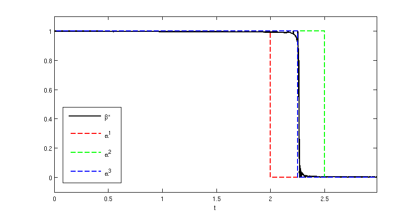
Figure 1. Optimal control for the relaxed problem and the integer control obtained by sum up rounding strategies for different $\Delta t$ for the test problem in Section 4.

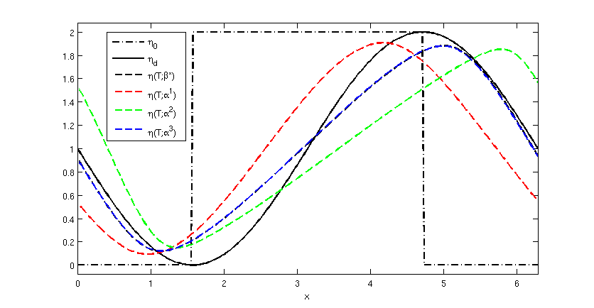
Figure 2. Initial data, the desired final time state and finial time plots of the solutions for the relaxed control and different integer controls for the test problem in Section 4.

5. Conclusions

Our analysis and numerical results show that certain PDE mixed-integer optimal control problems of hyperbolic type can be solved successfully und very efficiently using methods based on relaxation and rounding strategies.

References

• [1] Mapundi K. Banda and Michael Herty. Multiscale modeling for gas flow in pipe networks. Math. Methods Appl. Sci., 31(8):915–936, 2008.
• [2] Mapundi K. Banda and Michael Herty. Adjoint IMEX-based schemes for control problems governed by hyperbolic conservation laws. Comput. Optim. Appl., 51(2):909–930, 2012.
• [3] B.T. Baumrucker and L.T. Biegler. MPEC strategies for optimization of a class of hybrid dynamic systems. Journal of Process Control, 19(8):1248–1256, 2009. Special Section on Hybrid Systems: Modeling, Simulation and Optimization.
• [4] B.T. Baumrucker and L.T. Biegler. MPEC strategies for cost optimization of pipeline operations. Comput. Chem. Eng., 34(6):900–913, 2010.
• [5] Stefano Bianchini. A Glimm type functional for a special Jin-Xin relaxation model. Ann. Inst. H. Poincaré Anal. Non Linéaire, 18(1):19–42, 2001.
• [6] Alberto Bressan. Hyperbolic systems of conservation laws, volume 20 of Oxford Lecture Series in Mathematics and its Applications. Oxford University Press, Oxford, 2000. The one-dimensional Cauchy problem.
• [7] I. Capuzzo-Dolcetta and L. C. Evans. Optimal switching for ordinary differential equations. SIAM J. Control Optim., 22(1):143–161, 1984.
• [8] R. Courant and D. Hilbert. Methods of mathematical physics. Vol. II. Wiley Classics Library. John Wiley & Sons, Inc., New York, 1989. Partial differential equations, Reprint of the 1962 original, A Wiley-Interscience Publication.
• [9] Björn Geißler, Antonio Morsi, and Lars Schewe. A new algorithm for MINLP applied to gas transport energy cost minimization. In Facets of combinatorial optimization, pages 321–353. Springer, Heidelberg, 2013.
• [10] Matthias Gerdts. A variable time transformation method for mixed-integer optimal control problems. Optimal Control Appl. Methods, 27(3):169–182, 2006.
• [11] Simone Göttlich, Michael Herty, and Ute Ziegler. Modeling and optimizing traffic light settings in road networks. Comput. Oper. Res., 55:36–51, 2015.
• [12] Simon Haller and Günther Hörmann. Comparison of some solution concepts for linear first-order hyperbolic differential equations with non-smooth coefficients. Publ. Inst. Math. (Beograd) (N.S.), 84(98):123–157, 2008.
• [13] F. M. Hante, G. Leugering, and T. I. Seidman. Modeling and analysis of modal switching in networked transport systems. Applied Mathematics and Optimization, 59(2):275–292, 2009.
• [14] Falk M. Hante and Sebastian Sager. Relaxation methods for mixed-integer optimal control of partial differential equations. Comput. Optim. Appl., 55(1):197–225, 2013.
• [15] A. Heygi, B. De Schutter, and J. Hellendoorn. Optimal coordination of variable speed limits to suppress shock waves. IEEE Transactions on Intelligent Transportation Systems, 6(1):102–112, 2005.
• [16] M. Hinze, R. Pinnau, M. Ulbrich, and S. Ulbrich. Optimization with PDE constraints, volume 23 of Mathematical Modelling: Theory and Applications. Springer, New York, 2009.
• [17] Shi Jin and Zhou Ping Xin. The relaxation schemes for systems of conservation laws in arbitrary space dimensions. Comm. Pure Appl. Math., 48(3):235–276, 1995.
• [18] Michael N. Jung, Christian Kirches, and Sebastian Sager. On perspective functions and vanishing constraints in mixed-integer nonlinear optimal control. In Facets of combinatorial optimization, pages 387–417. Springer, Heidelberg, 2013.
• [19] Christian Kirches. Personal communication (07/2015).
• [20] Pierre-Olivier Lamare, Antoine Girard, and Christophe Prieur. Switching rules for stabilization of linear systems of conservation laws. SIAM J. Control Optim., 53(3):1599–1624, 2015.
• [21] H. W. J. Lee, K. L. Teo, V. Rehbock, and L. S. Jennings. Control parametrization enhancing technique for optimal discrete-valued control problems. Automatica J. IFAC, 35(8):1401–1407, 1999.
• [22] Michael Oberguggenberger. Propagation of singularities for semilinear hyperbolic initial-boundary value problems in one space dimension. J. Differential Equations, 61(1):1–39, 1986.
• [23] Marc E. Pfetsch, Armin Fügenschuh, Björn Geißler, Nina Geißler, Ralf Gollmer, Benjamin Hiller, Jesco Humpola, Thorsten Koch, Thomas Lehmann, Alexander Martin, Antonio Morsi, Jessica Rövekamp, Lars Schewe, Martin Schmidt, Rüdiger Schultz, Robert Schwarz, Jonas Schweiger, Claudia Stangl, Marc C. Steinbach, Stefan Vigerske, and Bernhard M. Willert. Validation of nominations in gas network optimization: models, methods, and solutions. Optim. Methods Softw., 30(1):15–53, 2015.
• [24] Sebastian Sager, Hans Georg Bock, and Moritz Diehl. The integer approximation error in mixed-integer optimal control. Math. Program., 133(1-2, Ser. A):1–23, 2012.
• [25] Sebastian Sager, Michael Jung, and Christian Kirches. Combinatorial integral approximation. Math. Methods Oper. Res., 73(3):363–380, 2011.
• [26] Jiong Min Yong. Optimal switching and impulse controls for distributed parameter systems. Systems Sci. Math. Sci., 2(2):137–160, 1989.