Asynchronous Networks and Event Driven Dynamics

Abstract.

Real-world networks in technology, engineering and biology often exhibit dynamics that cannot be adequately reproduced using network models given by smooth dynamical systems and a fixed network topology. Asynchronous networks give a theoretical and conceptual framework for the study of network dynamics where nodes can evolve independently of one another, be constrained, stop, and later restart, and where the interaction between different components of the network may depend on time, state, and stochastic effects. This framework is sufficiently general to encompass a wide range of applications ranging from engineering to neuroscience. Typically, dynamics is piecewise smooth and there are relationships with Filippov systems. In the first part of the paper, we give examples of asynchronous networks, and describe the basic formalism and structure. In the second part, we make the notion of a functional asynchronous network rigorous, discuss the phenomenon of dynamical locks, and present a foundational result on the spatiotemporal factorization of the dynamics for a large class of functional asynchronous networks.

1. Introduction

In this work we develop a theory of asynchronous networks and event driven dynamics. This theory constitutes an approach to network dynamics that takes account of features encountered in networks from modern technology, engineering, and biology, especially neuroscience. For these networks dynamics can involve a mix of distributed and decentralized control, adaptivity, event driven dynamics, switching, varying network topology and hybrid dynamics (continuous and discrete). The associated network dynamics will generally only be piecewise smooth, nodes may stop and later restart and there may be no intrinsic global time (we give specific examples and definitions later). Significantly, many of these networks have a function. For example, transportation networks bring people and goods from one point to another and neural networks may perform pattern recognition or computation.

Given the success of network models based on smooth differential equations and methods based on statistical physics, thermodynamic formalism and averaging (which typically lead to smooth network dynamics), it is not unreasonable to ask whether it is necessary to incorporate issues such as nonsmoothness in a theory of network dynamics. While nonsmooth dynamics is more familiar in engineering than in physics, we argue below that ideas from engineering, control and nonsmooth dynamics apply to many classes of network and that nonsmoothness often cannot be ignored in the analysis of network function. As part of these introductory comments, we also explain the motivation underlying our work, and describe one of our main results: the modularization of dynamics theorem.

Temporal averaging

Consider the analysis of a network where links are added and removed over time. Two extreme cases have been widely considered in the literature. If the network topology switches rapidly, relative to the time scale of the phenomenon being considered, then we may be able to replace the varying topology by the time-averaged topology. Providing that the network topology is not state dependent, the resulting dynamics will typically be smooth. On the other hand, if the topology changes slowly enough relative to the time scale of interest, we may regard the topology as constant and again we obtain smooth network dynamics. Either one of these approaches may be applicable in a system where time scales are clearly separated.

However, in many situations, especially those involving control or close to bifurcation, changes in network topology may play a crucial role in network function and an averaging approach may fail or neglect essential structure. This is well-known for problems in optimized control where solutions are typically nonsmooth and averaging gives the wrong solutions (for example, in switching problems using thermostats). For an example with variable network topology, we cite the effects of changing connection structure (transmission line breakdown), or adding/subtracting a microgrid, on a power grid. Neither averaging nor the assumption of constant network structure are appropriate tools: we cannot average the problems away. Instead, we are forced to engage with an intermediate regime, where nonsmoothness (switching) and control play a crucial role in network function.

Spatial averaging and network evolution

Much current research on networks is related to the description and understanding of complex systems [7, 18, 44, 49]. Roughly speaking, and avoiding a formal definition [44], we regard a complex system as a large network of nonlinearly interacting dynamical systems where there are feedback loops, multiple time and/or spatial scales, emergent behaviour, etc. One established approach to complex networks and systems uses ideas from statistical mechanics and thermodynamic formalism. For example, models of complex networks of interconnected neurons can sometimes be described in terms of their information processing capability and entropy [58]. These methods originate from applications to large interacting systems of particles in physics. As Schrödinger points out in his 1943 Trinity College, Dublin, lectures [59]

“…the laws of physics and chemistry are statistical throughout.”

In contrast to the laws of physics and chemistry, evolution plays a decisive role in the development of complex biological structure. Functional biological structures that provided the basis for evolutionary development can be quite small – the nematode worm caenorhabditis elegans has 302 neurons. If the underlying small-scale structure still has functional relevance, an approach based on statistical averages to complex biological networks has to be limited; on the one hand, averaging over the entire network will likely ignore any small scale structure, and on the other hand statistical averages have little or no meaning for small systems – at least on a short time scale.

Reverse engineering large biological structures appears completely impractical; in part this is because of the role that evolution plays in the development of complex structure. Evolution works towards optimization of function, rather than simplicity, and is often local in character with the flavour of decentralized control. Similar issues arise in understanding evolved engineering structures. For example, the internal combustion engine of a car in 1950 was a simple device, whose operation was synchronized through mechanical means. A modern internal combustion engine is structurally complex and employs a mix of synchronous and asynchronous systems controlled by multiple computer processors, sensors and complex computer code.

Reductionism

In nonlinear network dynamics, and complex systems generally, there is the question as to how far one can make use of reductionist techniques [5], [44, 2.5]. One approach, advanced by Alon and Kastan [39] in biology, has been the identification and description of relatively simple and small dynamical units, such as non-linear oscillators or network motifs (small network configurations that occur frequently in large biological networks [18, Chapter 19]). Their premise is that a modular, or engineering, approach to network dynamics is feasible: identify building blocks, connect together to form networks and then describe dynamical properties of the resulting network in terms of the dynamics of its components.

“Ideally, we would like to understand the dynamics of the entire network based on the dynamics of the individual building blocks.” Alon [4, page 27].

While such a reductionist approach works well in linear systems theory, where a superposition principle holds, or in the study of synchronization in weakly coupled systems of nonlinear approximately identical oscillators [55, 56, 8, 32], it is usually unrealistic in the study of heterogenous networks modelled by a system of analytic nonlinear differential equations: network dynamics may bear little or no relationship to the intrinsic (uncoupled) dynamics of nodes.

A theory of asynchronous networks.

The theory of asynchronous networks we develop provides an approach to the analysis of dynamics and function in complex networks. We illustrate the setting for our main result with a simple example. Figure 1 shows the schematics of a network where there is only intermittent connection between nodes. We assume eight nodes $N_{1},\dotsc,N_{8}$. Each node $N_{i}$ will be given an initial state and started at time $T_{i}\geq 0$. Crucially, we assume the network has a function: reaching designated terminal states in finite time – indicated on the right hand side of the figure. Nodes interact depending on their state. For example, referring to figure 1, nodes $N_{1}$, $N_{2}$ first interact during the event indicated by $\mathbf{E}^{a}$. Observe there is no global time defined for this system but there is a partially ordered temporal structure: event $\mathbf{E}^{c}$ always occurs after event $\mathbf{E}^{a}$ but may occur before or after event $\mathbf{E}^{b}$. We caution that while the direction of time is from left-to-right, there is no requirement of moving from left to right in the spatial variables: the phase space dimension for nodes could be greater than one and the initialization and terminations sets could be the same. This example can be generalized to allow for changes in the number and type of nodes after each event. The intermittent connection structure we use may be viewed as an extension of the idea of conditional action as defined by Holland in the context of complex adaptive systems [36].

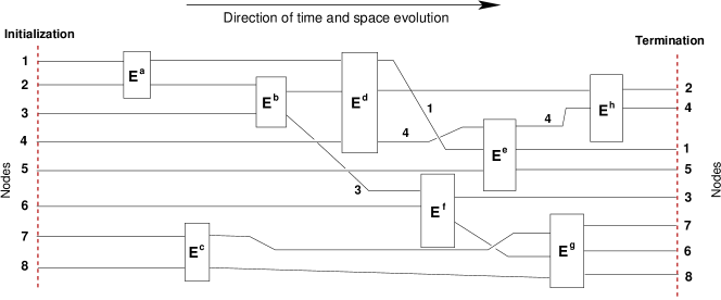
Figure 1. A functional feedforward network with 8 nodes

Our main result, stated and proved in part II of this work [13], is a modularization of dynamics theorem that yields a functional decomposition for a large class of asynchronous networks. Specifically, we give general conditions that enable us to represent a large class of functional asynchronous networks as feedforward functional networks of the type illustrated in figure 1. As a consequence, the function of the original network can be expressed explicitly in terms of uncoupled node dynamics and event function. Nonsmooth effects, such as changes in network topology through decoupling of nodes and stopping and restarting of nodes, are one of the crucial ingredients needed for this result. In networks modelled by smooth dynamical systems, all nodes are effectively coupled to each other at all times and information propagates instantly across the entire network. Thus, a spatiotemporal decomposition is only possible if the network dynamics is nonsmooth and (subsets of) nodes are allowed to evolve independently of each other for periods of time. This allows the identification of dynamical units, each with its own function, that together comprise the dynamics and function of the entire network. The result highlights a drawback of averaging over a network: the loss of information about the individual functional units, and their temporal relations, that yield network function.

A functional decomposition is natural from an evolutionary point of view: the goal of an evolutionary process is optimization of (network) function. Thus, rather than asking how network dynamics can be understood in terms of the dynamics of constituent subnetworks – the classical reductionist question – the issue is how network function can be understood in terms of the function of network constituents. Our result not only gives a satisfactory answer to Alon’s question for a large class of functional asynchronous networks but suggests an approach to determining key structural features of components of a complex system that is partly based on an evolutionary model for development of structure. Starting with a small well understood model, such as the class of functional feedforward networks described above, we propose looking at bifurcation in the context of optimising a network function – for example, understanding the effect on function when we break the feedforward structure by adding feedback loops.

Relations with distributed networks

An underlying theme and guide for our formulation and theory of asynchronous networks is that of efficiency and cost in large distributed networks. We recall the guidelines given by Tannenbaum & van Steen [61, page 11] for scalability in large distributed networks (italicised comments added):

• No machine has complete information about the (overall) system state. [communication limited]

• Machines make decisions based only on local information. [decentralized control]

• Failure of one machine does not ruin the algorithm. [redundancy]

• There is no implicit assumption of global time.

Of course, networks dynamics, in either technology, engineering or biology, is likely to involve a complex mix of synchronous and asynchronous components. In particular, timing (clocks, whether local or global) may be used to trigger the onset of events or processes as part of a weak mechanism for centralized control or resetting. Evolution is opportunistic – whatever works well will be adopted (and adapted) whether synchronous or asynchronous in character. In specific cases, especially in biology, it may be a matter of debate as to which viewpoint – synchronous or asynchronous – is the most appropriate. The framework we develop is sufficiently flexible to allow for a wide mix of synchronous and asynchronous structure at the global or local level.

Past work

Mathematically speaking, much of what we say has significant overlap with other areas and past work. We cite in particular, the general area of nonsmooth dynamics, Filippov systems and hybrid systems (for example, [27, 6, 50, 11]) and time dependent network structures (for example, [9, 47, 33, 37]). While the theory of nonsmooth dynamics focuses on problems in control, impact, and engineering, rather than networks, there is significant work studying bifurcation (for example [43, 10]) which is likely to apply to parts of the theory we describe. From a vast literature on networks and dynamics, we cite Newman’s text [52] for a comprehensive introduction to networks, and the very recent tutorial of Porter & Gleeson [57] which addresses questions related to our work, gives an overview and introduction to dynamics on networks, and includes an extensive bibliography of past work.

Outline of contents

After preliminaries in section 2, we give in section 3 vignettes (no technical details) of several asynchronous networks from technology, engineering, transport and neuroscience. In section 4, we give a mathematical formulation of an asynchronous network with a focus on event driven dynamics, and constraints. We follow in section 5 with two more detailed examples of asynchronous networks including an illuminating and simple example of a transport network which requires minimal technical background yet exhibits many characteristic features of an asynchronous network, and a discussion of power grid models that indicates both the limitations and possibilities of our approach. We conclude with a discussion of products of asynchronous networks in section 6 that illuminates some of the subtle features of the event map. In part II [13], we develop the theory of functional asynchronous networks and give the statement and proof of the modularization of dynamics theorem.

Dedication. The genesis of this paper lies in a visit in 2010 by one us (MF) to work with Dave Broomhead at Manchester University. Dave was very interested in asynchronous processes and local clocks. During the visit, he came up with a 2 cell random dynamical systems model for the investigation of asynchronous dynamics and local time. This 2 cell model provided the seed and stimulus for the work described in this paper. Dave’s illness and untimely death sadly meant that our planned collaboration on this work could not be realized.

2. Preliminaries and generalities on networks

2.1. Notational conventions

We recall a few mostly standard notational conventions used throughout. Let $\mathbb{N}$ denote the natural numbers (the strictly positive integers), $\mathbb{Z}_{+}$ denote the set of nonnegative integers, ${}_{+}=\left\{x\in\real\,|\,x\geq 0\right\}$, and $\real(>0)=\left\{x\in{}_{+}\,|\,x\neq 0\right\}$. Given $n\in\mathbb{N}$, define $\mathbf{n}=\left\{1,\dotsc,n\right\}$. Let ${\mathbf{n}}^{\bullet}=\left\{0,1,\dotsc,n\right\}$ and, more generally, for $A\subset\mathbb{N}$ define ${A}^{\bullet}=A\cup\left\{0\right\}$.

2.2. Network notation

We establish our conventions on network notation; we follow these throughout this work.

Suppose the network $\mathcal{N}$ has $k$ nodes, $N_{1},\dotsc,N_{k}$. Abusing notation, we often let $\mathcal{N}$ denote both network and the set of nodes $\{N_{1},\dotsc,N_{k}\}$. Denote the state or phase space for $N_{i}$ by $M_{i}$ and set $\mathbf{M}=\prod_{i\in\mathbf{k}}M_{i}$ – the network phase space. Denote the state of node $N_{i}$ by ${\mathbf{x}}_{i}\in M_{i}$ and the network state by $\mathbf{X}=({\mathbf{x}}_{1},\dotsc,{\mathbf{x}}_{k})\in\mathbf{M}$.

Smooth dynamics on $\mathcal{N}$ will be given by a system of ordinary differential equations (ODEs) of the form

(1) $${\mathbf{x}}_{i}^{\prime}=f_{i}({\mathbf{x}}_{i};{\mathbf{x}}_{j_{1}},\dotsc,{\mathbf{x}}_{j_{e_{i}}}),\;\;i\in\mathbf{k},$$

where the components $f_{i}$ are at least $C^{1}$ (usually $C^{\infty}$ or analytic) and the following conditions are satisfied.

(N1) For all $i\in\mathbf{k}$, $j_{1}<\dotsc<j_{e_{i}}$ are distinct elements of $\mathbf{k}\smallsetminus\{i\}$ (and so $e_{i}<k$).

Set $J(i)=\{j_{1},\dotsc,j_{e_{i}}\}\subset\mathbf{k}$, $i\in\mathbf{k}$ ($J(i)$ may be empty).

(N2) For each $i\in\mathbf{k}$, the evolution of $N_{i}$ depends nontrivially on the state of $N_{j}$, $j\in J(i)$, in the sense that there exists a choice of ${\mathbf{x}}_{i}\in M_{i}$ and ${\mathbf{x}}_{j_{s}}\in M_{j_{s}}$, $j_{s}\in J(i)\smallsetminus\{j\}$, such that $f_{i}({\mathbf{x}}_{i};{\mathbf{x}}_{j_{1}},\dotsc,{\mathbf{x}}_{j_{e_{i}}})$ is not constant as a function of ${\mathbf{x}}_{j}$.

(N3) We generally assume the evolution of $N_{i}$ depends on the state of $N_{i}$. If we need to emphasize that $f_{i}$ does not depend on ${\mathbf{x}}_{i}$ in the sense of (N2), we write $f_{i}({\mathbf{x}}_{j_{1}},\dotsc,{\mathbf{x}}_{j_{e_{i}}})$, if $J(i)\neq\emptyset$. If $J(i)=\emptyset$, we regard the dependence of $f_{i}$ on ${\mathbf{x}}_{i}$ as nontrivial iff $f_{i}$ is not identically zero and then write $f_{i}({\mathbf{x}}_{i})$. Otherwise $f_{i}\equiv 0$.

Remark 2.1.

Given network equations (1) which do not satisfy (N1–3), we can first redefine the $f_{i}$ so as to satisfy (N1). Next we remove trivial dependencies so as to satisfy (N2). Finally, we check for the dependence of $f_{i}$ on the internal state ${\mathbf{x}}_{i}$ and modify the $f_{i}$ as necessary to achieve (N3). If $f_{i}\equiv 0$, we can remove the node from the network. Consequently, it is no loss of generality to always assume that (N1–3) are satisfied, with $f_{i}\not\equiv 0$. A consequence is that any network vector field $\mathbf{f}=(f_{1},\dotsc,f_{k}):\mathbf{M}\rightarrow T\mathbf{M}$ can be uniquely written in the form (1) so as to satisfy (N1–3).

Let $M(k)$ denote the space of $k\times k$ $0$ -$1$ matrices $\beta=(\beta_{ij})_{i,j\in\mathbf{k}}$ with coefficients in $\left\{0,1\right\}$ and $\beta_{ii}=0$, all $i\in\mathbf{k}$. Each $\beta\in M(k)$ determines uniquely a directed graph $\Gamma_{\beta}$ with vertices $N_{1},\dotsc,N_{k}$ and directed edge $N_{j}\rightarrow N_{i}$ iff $\beta_{ij}=1$ and $i\neq j$. The matrix $\beta$ is the adjacency matrix of $\Gamma_{\beta}$. We refer to $\beta$ as a connection structure on $\mathcal{N}$.

If $\mathbf{f}:\mathbf{M}\rightarrow T\mathbf{M}$ is a network vector field satisfying (N1–3), then $\mathbf{f}$ determines a unique connection structure $C(\mathbf{f})\in M(k)$ with associated graph $\Gamma_{C(\mathbf{f})}$. In order to specify the graph uniquely, it suffices to specify the set of directed edges.

We define the network graph $\Gamma=\Gamma(\mathcal{N},\mathbf{f})$ to be the directed graph $\Gamma_{C(\mathbf{f})}$. Thus, $\Gamma(\mathcal{N},\mathbf{f})$ has node set $\mathcal{N}=\{N_{1},\dotsc,N_{k}\}$ and a directed connection $N_{j}\rightarrow N_{i}$ will be an edge of $\Gamma$ if and only if $j\neq i$ and the dynamical evolution of $N_{i}$ depends nontrivially on the state of $N_{j}$.

Remark 2.2.

Our conventions are different from formalisms involving multiple edge types (for example, see [32, 3] for continuous dynamics and [1] for discrete dynamics). We allow at most one connection between distinct nodes of the network graph and do not use self-loops: connections encode dependence.

2.2.1. Additive input structure

In many cases of interest, we have an additive input structure [26] and the components $f_{i}$ of $\mathbf{f}$ may be written

(2) $$f_{i}({\mathbf{x}}_{i};{\mathbf{x}}_{j_{1}},\dotsc,{\mathbf{x}}_{j_{e_{i}}})=F_{i}({\mathbf{x}}_{i})+\sum_{s=1}^{e_{i}}F_{ij_{s}}({\mathbf{x}}_{j_{s}},{\mathbf{x}}_{i}),\;i\in\mathbf{k}.$$

Additive input structure implies that there are no interactions between inputs $N_{j},N_{k}\rightarrow N_{i}$, as long as $j,k\neq i$, $j\neq k$, and allows us to add and subtract inputs and nodes in a consistent way. We may think of ${\mathbf{x}}_{i}^{\prime}=F_{i}({\mathbf{x}}_{i})$ as defining the intrinsic dynamics of the node.

Remarks 2.3.

(1) Additive input structure is usually assumed for modelling weakly coupled nonlinear oscillators and is required for reduction to the standard Kuramoto phase oscillator model [42, 25, 38].
(2) If we identify a null state ${\mathbf{z}}_{j}^{\star}$ for each node $N_{j}$, then the decomposition (2) will be unique if we require $F_{ij}({\mathbf{z}}_{j}^{\star},{\mathbf{x}}_{i})\equiv 0$. If a node is in the null state then it has no output to other nodes and is ‘invisible’ to the rest of the network. If we have an additive structure on the phase spaces $M_{i}$ (for example, each $M_{i}$ is a domain in ⁿ or an $n$-torus $\mathbb{T}^{n}$) it is natural to take ${\mathbf{z}}_{i}^{\star}=0$.
(3) If $M_{i}={}^{n}$ or $\mathbb{T}^{n}$, $i\in\mathbf{k}$, and $F_{ij_{s}}({\mathbf{x}}_{j_{s}},{\mathbf{x}}_{i})=G_{ij_{s}}({\mathbf{x}}_{j_{s}}-{\mathbf{x}}_{i})$, $i,j_{s}\in\mathbf{k}$, the coupling is diffusive (see [1, §2.5] for general phase spaces).

2.3. Synchronous networks

Systems of ordinary differential equations like (1) give mathematical models for synchronous networks. By synchronous, we mean nodes are all synchronized to a global clock – the terminology comes from computer science. Indeed, if each node comes with a local clock, then all the clocks can be set to the same time provided that the network is connected (we ignore the issue of delays, but see [45]). The synchronization of local clocks is essentially forced by the model and the connectivity of the network graph; nodes cannot evolve independently of one another unless the network is disconnected.

We recall some characteristic features of synchronous networks.

Global evolution:

Nodes never evolve independently of each other: if the state of any node is perturbed, then generically the evolution of the states of the remaining nodes changes.

Stopped nodes:

If a node (or subset of node variables) is at equilibrium or “stopped” for a period of time, it will remain stopped for all future time. If a node has a non-zero initialization, it will never stop (in finite time).

Fixed connection structure:

The connection structure of a synchronous network is fixed: it does not vary in time and is not dependent on node states: one system of ODEs suffices to model network dynamics.

Reversibility:

Solutions are uniquely defined in backward time.

3. Asynchronous networks: examples

In this section, we give several vignettes of asynchronous networks that illustrate the main features differentiating them from synchronous networks. We amplify two of these examples in section 5 after we have developed our basic formalism for asynchronous networks.

Example 3.1 (Threaded and parallel computation).

Threaded or parallelized computation provides an example of a discrete stochastic asynchronous network. Computation based on a single processor (or single core of a processor) proceeds synchronously and sequentially. The speed of the computation is dependent on the clock speed of the processor as the processor clock synchronizes the various steps in the computation. In threaded or parallel computation, computation is broken into blocks or ‘threads’ which are then computed independently of each other at a rate that is partly dependent on the clock rates of the processors involved in the computation (these need not be identical). At certain points in the computation, threads need to exchange information with other threads. This process involves stopping and synchronizing (updating) the thread states: a thread may have to stop and wait for other threads to complete their computations and update data before it can continue with its own computation.

Threaded computation is non-deterministic: the running and stopping times of each thread are unpredictable and differ from run to run.

Each thread has its own clock (determined by its associated processor). Threads will be unaware of the clock times of other threads except during the stopping and synchronization events which can be managed synchronously (central control) or asynchronously (local control).

This example shows many characteristic features of an asynchronous network: nodes (threads) evolving independently of each other, and stopping, synchronization and restarting events. The network also has a function – transforming a set of initial data into a set of final data in finite time – and there is the possibility of incorrect code that can lead to a process that stops before the computation is complete (a deadlock), or errors where threads try to access a resource at the same time (race condition). $\diamondsuit$

Example 3.2 (Power grids & microgrids).

A power grid consists of a connected network of various types of generators and loads connected by transmission lines. A critical issue for the stability of the power grid is maintaining tight voltage frequency synchronization across the grid in the presence of voltage phase differences between generators and loads and variation in generator outputs and loads. We refer to Kundur [40] for classical power grid theory, Dörfler et al. [23] or Nishikawa & Motter [53], for some more recent and mathematical perspectives, and [41] for general issues and definitions on power system stability.

Historically, power grids have been centrally controlled and one of the main stability issues has been the effect on stability of a sudden change in structure – such as the removal of a transmission line, breakdown of a generator or big change in load. Detailed models of the power grid need to account for a complex multi-timescale stiff system. Typically stability has been analyzed using numerical methods. However, relatively simple classes of network models for power grids based on frequency and phase synchronization have been developed which are applicable for the analysis of some stability and control issues, especially those described in the next paragraph. We describe these models in more technical detail in section 5.

Interest has recently focused on renewable (small) energy sources in a power grid (for example, wind and solar power) and how to integrate microgrids based on renewable sources into the power grid using a mix of centralized and decentralized control. Concurrent with this interest is the issue of smart grids: modifying local loads in terms of the availability and real time costs of power. While the classical power grid model is of a synchronous network, though with asynchronous features such as the effects on stability of the breakdown of a connection (transmission line), these problems focus on asynchronous networks. For example, given a microgrid with renewable energy sources such as wind and solar, time varying loads and buffers (large capacity batteries), how can the microgrid be switched in and out of the main power grid while maintaining overall system stability? In this case, switching will be determined by state (for example, frequency changes in the main power grid signifying changes in power demand or changes in the output of renewable sources or battery reserves) and stochastic effects (resulting, for example, from load changes and the incorporation of smart grid technology). This is already a tricky problem of distributed and decentralized control with just one microgrid; in the presence of many microgrids there is the potential problem of synchronization of switching microgrids in and out of the main power grid. Similar problems occur in smart grids [62].

Asynchronous features of power grid networks include variation in connection and node structure (separation, or islanding, of microgrids from main power grid), state dependence of connection structure, synchronization and restarting events (during incorporation of microgrid into main grid). $\diamondsuit$

Example 3.3 (Thresholds, spiking networks and adaptation).

Many mathematical models from engineering and biology incorporate thresholds. For networks, when a node attains a threshold, there are often changes (addition, deletion, weights) in connections to another nodes. For networks of neurons, reaching a threshold can result in a neuron firing (spiking) and short term connections to other neurons (for transmission of the spike). For learning mechanisms, such as Spike-Timing Dependent Plasticity (STDP) [29] relative timings (the order of firing) are crucial [30, 17, 51] and so each neuron, or connection between a pair of neurons, comes with a ‘local clock’ that governs the adaptation in STDP. In general, networks with thresholds, spiking and adaptation provide characteristic examples of asynchronous networks where dynamics is piecewise smooth and hybrid – a mix of continuous and discrete dynamics. Spiking networks also highlight the importance of efficient communication in large networks: spiking induced connections between neurons are brief and low cost. There is also no oscillator clock governing all computations along the lines of a single processor computer. These examples all fit well into the framework of asynchronous networks but, on account of the background knowledge required, we develop the theory and formalism elsewhere [14]. $\diamondsuit$

Example 3.4 (Transport & production networks).

We discuss transport networks first. For simplicity, we work with a single transport mode: trains. Typically, trains have to be scheduled to be in a station for overlapping times (stopping, restarting, connections and local times) so that passengers can transfer between trains, or stop in a passing loop (so that trains can pass on a single track line). In addition, a train can divide into two parts or two trains can be combined (variation in node structure, stopping and synchronization event). Generally, transport networks will have asynchronous features and exhibit state dependent connection structure, local times and have a strong stochastic component (for example, in stopping and restarting times). We develop a simple formal transport model in section 5 (and in part II [13]) that illustrates basic ideas and results in the theory of asynchronous networks but does not require extensive background knowledge.

A simple example of a production network is a paint mixer. Assume a controller which accepts inputs – requested colour – which, after computation to find tint weights (‘tint code’), signals a request to inject selected tints according to the tint code into the base paint which is then mixed. The output is a can of coloured and fully mixed paint. Dynamics plays a limited role – except possibly at the mixing stage (for example, if there is a sensor that can detect an acceptable level of mixing). For this network, there is a varying connection structure determined by the signalling and tint injection. A characteristic feature of this, and many production networks, is the large variation in time scales. Signalling will typically be very fast, injection moderately fast and mixing rather slow. If the times of inputs to the controller are stochastic (for example, follow a Poisson process), then there will be issues of queueing and prioritization of inputs. If it is intended to maximize usage of the production facilities and avoid long waits, then it is natural to suppose that there are several mixing units and the output of the tint units is switched between mixer units according to their availability. Of course, the paint mixer may be a small part of a much larger distributed production network for which we can expect multiple time scales, switching between production units, changing the output of production units, stopping or restarting units, etc. The control of large distributed production systems will typically involve a mix of decentralized and centralized control.

Synthesis of proteins at the cellular level can be viewed as a generalization of the paint mixer model. We refer the reader to Alon [4, 8, Chapter 1] for background and more details, especially on transcription networks. $\diamondsuit$

We summarize some of the key features of asynchronous networks illustrated by all of the preceeding examples.

1. Variable connection structure and dependencies between nodes. Changes in connection structure may depend on the state of the system or be given by a stochastic process.

2. Synchronization events associated with stopping or waiting states of nodes.

3. Order of events may depend on the initialization of the system or stochastic effects.

4. Dynamics is only piecewise smooth and there may be a mix of continuous and discrete dynamics.

5. Aspects involving function, adaptation and control.

6. Evolution only defined for forward time – systems are non-reversible.

4. A Mathematical model for asynchronous networks

In this section we formalize the notion of an asynchronous network. Our focus is on deterministic (not stochastic) and continuous time asynchronous networks which are autonomous (no explicit dependencies on time) and we use the term ‘asynchronous network’ as synonym for a deterministic and autonomous continuous time asynchronous network.

4.1. Basic formalism for asynchronous networks

Consider a network $\mathcal{N}$ with $k$ nodes, $N_{1},\dotsc,N_{k}$, and follow the conventions of section 2: each node $N_{i}$ has phase space $M_{i}$, and $\mathbf{M}=\prod_{i=1}^{k}M_{i}$ – the network phase space. A network vector field $\mathbf{f}$ on $\mathbf{M}$ is assumed to satisfy conditions (N1–3) and so determines a unique connection structure $C(\mathbf{f})\in M(k)$ and associated network graph $\Gamma_{C(\mathbf{f})}$ (no self-loops).

Stopping, waiting, and synchronization are characteristic features of asynchronous networks. If nodes of a network are stopped or partially stopped, then node dynamics will be constrained to subsets of node phase space. We codify this situation by introducing a constraining node $N_{0}$ that, when connected to $N_{i}$, implies that dynamics on $N_{i}$ is constrained. We give the precise definition of constraint shortly (in 4.3); for the present, the reader may regard a constrained node as stopped – node dynamics is defined by the zero vector field. We only allow connections $N_{0}\rightarrow N_{i}$, $i\in\mathbf{k}$, and do not consider connections $N_{i}\rightarrow N_{0}$, $i\in\mathbf{k}^{\bullet}$. Henceforth we usually always assume there is a constraining node and let $\mathcal{N}=\left\{N_{0},N_{1},\dotsc,N_{k}\right\}$ denote the set of nodes. We emphasize that the constraining node $N_{0}$ has no dynamics and no associated phase space. In a network with no constraints (there are no connections $N_{0}\rightarrow N_{i}$), the constraining node $N_{0}$ plays no role and can be omitted. If we allow constraints, there may be more than one type of constraint on a node $N_{i}$.

Suppose that there are $p_{i}\in\mathbb{N}$ different constraints on the node $N_{i}$, $i\in\mathbf{k}$. Set $\mathbf{P}=(p_{1},\dotsc,p_{k})\in\mathbb{Z}_{+}^{k}$ and let $M_{\bullet}(k;\mathbf{P})$ denote the space of $k\times(k+1)$ matrices $\alpha=(\alpha_{ij})_{i\in\mathbf{k},j\in{\mathbf{k}}^{\bullet}}$ such that

1. $(\alpha_{ij})_{i,j\in\mathbf{k}}\in M(k)$ (and so $\alpha_{ii}=0,i\in\mathbf{k}$).

2. $\alpha_{i0}\in\mathbf{p}_{i}^{\bullet}$, $i\in\mathbf{k}$.

If $\alpha\in M_{\bullet}(k;\mathbf{P})$, we define the directed graph $\Gamma_{\alpha}$ by

1. $\Gamma_{\alpha}$ has node set $\mathcal{N}$.

2. For all $i,j\in\mathbf{k}$, $N_{j}\to N_{i}$ is an edge iff $\alpha_{ij}=1$.

3. $N_{0}\rightarrow N_{i}$ is an edge iff $\alpha_{i0}\neq 0$. We write $N_{0}\stackrel{{\scriptstyle\ell}}{{\rightarrow}}N_{i}$ if we need to specify the constraint corresponding to $\ell\in\mathbf{p}_{i}$.

We usually abbreviate $M_{\bullet}(k;\mathbf{P})$ to $M_{\bullet}(k)$. Let ${\boldsymbol{\emptyset}}\in M_{\bullet}(k)$ denote the empty connection structure (no edges).

If $\alpha\in M_{\bullet}(k)$, let $\alpha^{0}$ denote the first column $(\alpha_{i0})_{i\in\mathbf{k}}$ of $\alpha$. We have a natural projection $\pi:M_{\bullet}(k)\rightarrow M(k)$; $\alpha\mapsto\alpha^{\flat}$, defined by omitting the column $\alpha^{0}$. We write $\alpha\in M_{\bullet}(k)$ uniquely as

$$\alpha=(\alpha^{0}\,|\,\alpha^{\flat}).$$

The column vector $\alpha^{0}$ codifies the connections from the constraining node and $\alpha^{\flat}$ encodes the connections between the nodes $\{N_{1},\dotsc,N_{k}\}$.

Let $\alpha\in M_{\bullet}(k)$. We provisionally define an $\alpha$-admissible vector field $\mathbf{f}=(f_{1},\dotsc,f_{k})$ to be a network vector field such that for $i,j\in\mathbf{k}$, $i\neq j$, $f_{i}$ depends on the state ${\mathbf{x}}_{j}$ of $N_{j}$ iff $\alpha_{ij}=1$. If there is a connection $N_{0}\rightarrow N_{i}$ ($\alpha_{i0}\neq 0$), then there is a nontrivial constraint on $N_{i}$. An $\alpha$-admissible vector field has constrained dynamics if there are connections from the constraining node. If $\alpha={\boldsymbol{\emptyset}}$, nodes are uncoupled and unconstrained.

Definition 4.1.

(Notation and assumptions as above.)

1. A generalized connection structure $\mathcal{A}$ is a (nonempty) set of connection structures on $\mathcal{N}$.

2. An $\mathcal{A}$-structure $\mathcal{F}$ is a set $\mathcal{F}=\{\mathbf{f}^{\alpha}\,|\,\alpha\in\mathcal{A}\}$ of network vector fields such that each $\mathbf{f}^{\alpha}\in\mathcal{F}$ is $\alpha$-admissible.

Interactions between nodes in asynchronous networks may vary and can be state or time dependent or both. We focus on state dependence and assume interactions and constraints are determined by the state of the network through an event map $\mathcal{E}:\mathbf{M}\rightarrow\mathcal{A}$.

Definition 4.2.

Given a network $\mathcal{N}$, generalized connection structure $\mathcal{A}$, $\mathcal{A}$-structure $\mathcal{F}$, and surjective event map $\mathcal{E}:\mathbf{M}\rightarrow\mathcal{A}$, the quadruple $\mathfrak{N}=(\mathcal{N},\mathcal{A},\mathcal{F},\mathcal{E})$ defines an asynchronous network.

The network vector field of $\mathfrak{N}$ is given by the state dependent vector field $\mathbf{F}:\mathbf{M}\rightarrow T\mathbf{M}$ defined by

$$\mathbf{F}(\mathbf{X})=\mathbf{f}^{\mathcal{E}(\mathbf{X})}(\mathbf{X}),\;\mathbf{X}\in\mathbf{M}.$$

Remarks 4.3.

(1) Subject to simple regularity conditions, which we give later, the network vector field $\mathbf{F}$ will have a uniquely defined semiflow.
(2) In the sequel we often use the notation $\mathfrak{N}$ as shorthand for the asynchronous network $(\mathcal{N},\mathcal{A},\mathcal{F},\mathcal{E})$ (by extension, $\mathfrak{N}^{a}$ will be shorthand for $(\mathcal{N}^{a},\mathcal{A}^{a},\mathcal{F}^{a},\mathcal{E}^{a})$, etc.).

Example 4.4.

Let $k=2$ and $M_{1}=M_{2}=\real\times\mathbb{T}$. Suppose that dynamics of the uncoupled node $N_{i}$ is given by the smooth vector field $V_{i}(x_{i},\theta_{i})=(f_{i}(x_{i}),\omega_{i})$, where $f_{i}(0)\neq 0$, $\omega_{i}\in\real$, $i\in\mathbf{2}$.

Assume constrained dynamics for either node is defined on the invariant circle $\{0\}\times\mathbb{T}\subset\real\times\mathbb{T}$ by the vector field $Z_{i}(x_{i},\theta_{i})=(0,\omega_{i})$, $i\in\mathbf{2}$. When both nodes are constrained ($x_{1}=x_{2}=0$), assume (constrained) coupling is defined by the vector field $H=(H_{1},H_{2})$, where

$$H_{1}(x_{1},\theta_{1},x_{2},\theta_{2}) = (0,\omega_{1}+h(\theta_{2}-\theta_{1}))$$

$$H_{2}(x_{1},\theta_{1},x_{2},\theta_{2}) = (0,\omega_{2}+h(\theta_{1}-\theta_{2})),$$

and $h:\mathbb{T}\rightarrow\real$ is smooth. The 2-tori $\{(x_{1},x_{2})\}\times\mathbb{T}^{2}$ are invariant by the flow of $H$ for all $(x_{1},x_{2})\in{}^{2}$. Revert to standard (uncoupled and unconstrained) dynamics when $|\theta_{1}-\theta_{2}|\leq\varepsilon$, where $0<\varepsilon\ll 1$. We describe the network dynamics using asynchronous network formalism.

Take the generalized connection structure $\mathcal{A}=\{{\boldsymbol{\emptyset}},\alpha_{1},\alpha_{2},\beta\}$, where $\alpha_{i}=N_{0}\rightarrow N_{i}$, $i\in\mathbf{2}$, and $\beta=N_{0}\rightarrow N_{1}\leftrightarrow N_{2}\leftarrow N_{0}$.

Take $\mathcal{F}=\{\mathbf{f}^{\gamma}\,|\,\gamma\in\mathcal{A}\}$, where

$$\mathbf{f}^{\boldsymbol{\emptyset}}=(V_{1},V_{2}),\;\mathbf{f}^{\alpha_{1}}=(Z_{1},V_{2}),\;\mathbf{f}^{\alpha_{2}}=(V_{1},Z_{2}),\;\mathbf{f}^{\beta}=(H_{1},H_{2}).$$

Define the event map $\mathcal{E}:(\real\times\mathbb{T})^{2}\rightarrow\mathcal{A}$ by

$$\mathcal{E}(0,\theta_{1},0,\theta_{2}) = \beta,\;\text{if }|\theta_{1}-\theta_{2}|>\varepsilon$$

$$= {\boldsymbol{\emptyset}},\;\text{if }|\theta_{1}-\theta_{2}|\leq\varepsilon$$

$$\mathcal{E}(0,\theta_{1},x_{2},\theta_{2}) = \alpha_{1},\;\text{if }x_{2}\neq 0$$

$$\mathcal{E}(x_{1},\theta_{1},0,\theta_{2}) = \alpha_{2},\;\text{if }x_{1}\neq 0$$

$$\mathcal{E}(x_{1},\theta_{1},x_{2},\theta_{2}) = {\boldsymbol{\emptyset}},\;\text{if }x_{1}x_{2}\neq 0.$$

Network dynamics is given by the vector field $\mathbf{F}(\mathbf{X})=\mathbf{f}^{\mathcal{E}(\mathbf{X})}(\mathbf{X})$. Trajectories for $\mathbf{F}$ are built from pieces of the trajectories of $\mathbf{f}^{\boldsymbol{\emptyset}}$, $\mathbf{f}^{\alpha_{1}}$, $\mathbf{f}^{\alpha_{2}}$, and $\mathbf{f}^{\beta}$. Using the condition $f_{i}(0)\neq 0$, $i\in\mathbf{2}$, we see easily that $\mathbf{F}$ has a well-defined semiflow $\Phi_{t}(x_{1},\theta_{1},x_{2},\theta_{2})$, which is continuous in time $t\geq 0$ but is not necessarily continuous in $(x_{1},\theta_{1},x_{2},\theta_{2})$. $\diamondsuit$

4.2. Local foliations

Conditions for a constrained node $N_{i}$ will be given in terms of foliations of open subsets of $M_{i}$. We start by recalling basic definitions on foliations (see [46] for a detailed review).

A $p$-dimensional smooth (always $C^{\infty}$ here) foliation $\mathcal{L}$ of the $m$-dimensional manifold $W$ consists of a partition $\{L_{\alpha}\,|\,\alpha\in\Lambda\}$ of $W$ into connected sets, called leaves, such that for every $x\in W$, we can choose an open neighbourhood $U$ of $x$ and smooth embedding $\psi:U\rightarrow{}^{m}$ such that for each leaf $L_{\alpha}$, the components of $\phi(L_{\alpha}\cap U)$ are given by equations $x^{p+1}=\text{constant},\ldots,x^{m}=\text{constant}$. Each leaf of a foliation will be an immersed $p$-dimensional submanifold of $W$. For our applications, we always assume leaves are properly embedded closed submanifolds of $W$, $p<m$, and that the manifold $W$ has finitely many connected components. In general, a smooth foliation of the manifold $W$ will consist of a smooth foliation of each connected component of $W$ such that the dimension of leaves is constant on each connected component of $W$.

Examples 4.5.

(1) Every smooth nonsingular vector field on $W$ defines a 1-dimensional smooth foliation of $W$ (“flow-box” theorem of dynamical systems). The leaves are trajectories of the vector field.
(2) If $W=A\times B$, where $A$ and $B$ are manifolds, we have the product foliations $\mathcal{L}(A)$ and $\mathcal{L}(B)$ of $W$ defined by $\mathcal{L}(A)=\{A\times\{b\}\,|\,b\in B\}$ and $\mathcal{L}(B)=\{\{a\}\times B\,|\,a\in A\}$. Each leaf $\mathcal{L}(A)$ is transverse to every leaf of $\mathcal{L}(B)$. More generally, foliations $\mathcal{L},\mathcal{L}^{\prime}$ are transverse if leaves are transverse. A foliation of $W$, even by compact 1-dimensional leaves, need not have a transverse foliation. The best-known example is the Hopf fibration which defines a foliation of $S^{3}$ into circles. $\diamondsuit$

Suppose that $\mathcal{L}$ is a $p$-dimensional smooth foliation of $W$ with leaves $\left\{L_{\alpha}\,|\,\alpha\in\Lambda\right\}$. The tangent bundle along the foliation $\tau:\mathbb{L}\rightarrow W$ is the smooth vector sub-bundle of the tangent bundle $TW$ of $W$ defined by

$$\mathbb{L}=\bigcup_{x\in L_{\alpha},\,\alpha\in\Lambda}T_{x}L_{\alpha}\subset TW.$$

4.3. Constrained nodes and admissible vector fields

Following section 4.1, we assume $\mathcal{N}=\{N_{0},N_{1},\dotsc,N_{k}\}$, where the nodes $N_{i}$ have phase space $M_{i}$, $i\in\mathbf{k}$. Fix a $k$-tuple $\mathbf{P}=(p_{1},\dotsc,p_{k})\in\mathbb{Z}_{+}^{k}$. In what follows, we assume $\mathbf{P}\neq\mathbf{0}$.

Definition 4.6.

(Notation and assumptions as above.) A family $\mathbf{C}=\{(\mathbf{W}_{i},\boldsymbol{\mathcal{L}}_{i})\,|\,i\in\mathbf{k}\}$ is a constraint structure on $\mathcal{N}$ if, for all $i\in\mathbf{k}$ with $p_{i}>0$,

1. $\mathbf{W}_{i}=\{W_{i}^{\ell}\,|\,\ell\in\mathbf{p_{i}}\}$ is a family of nonempty open subsets of $M_{i}$.

2. $\boldsymbol{\mathcal{L}}_{i}=\{\mathcal{L}_{i}^{\ell}\,|\,\ell\in\mathbf{p_{i}}\}$, where $\mathcal{L}_{i}^{\ell}$ is a smooth foliation of $W_{i}^{\ell}$.

Remarks 4.7.

(1) If $p_{i}=0$, there are no constraints on $N_{i}$.
(2) If $p_{i}=1$, we set $\mathbf{W}_{i}=(W_{i},\mathcal{L}_{i})$ and $\mathcal{L}_{i}$ is a smooth foliation of the nonempty open subset $W_{i}$ of $M_{i}$. If we allow the dimension of leaves to vary between different connected components, and the families $\mathbf{W}_{i}$ to consist of disjoint open subsets of $M_{i}$, $i\in\mathbf{k}$, then we can reduce to the case $p_{i}\leq 1$ by taking $W_{i}=\bigcup_{\ell}W_{i}^{\ell}$ and $\mathcal{L}_{i}$ to be the foliation determined on $W_{i}$ by $\mathcal{L}_{i}|W_{i}^{\ell}=\mathcal{L}_{i}^{\ell}$, $\ell\in\mathbf{p_{i}}$. For our applications, it is no loss of generality to assume that $\mathbf{W}_{i}$ always consists of disjoint open subsets of $M_{i}$, $i\in\mathbf{k}$.

We can now give a precise definition of an $\alpha$-admissible vector field when there are constraints.

Definition 4.8.

Fix a constraint structure $\mathbf{C}=\{(\mathbf{W}_{i},\boldsymbol{\mathcal{L}}_{i})\,|\,i\in\mathbf{k}\}$ on $\mathcal{N}$ and let $\alpha\in M_{\bullet}(k)$. A smooth vector field $\mathbf{f}=(f_{1},\dotsc,f_{k})$ on $\mathbf{M}$ is an $\alpha$-admissible vector field if

1. For $i,j\in\mathbf{k}$, $i\neq j$, $f_{i}$ depends on $\mathbf{x}_{j}$ iff $\alpha_{ij}=1$.

2. If $\alpha_{i0}=\ell>0$, then $f_{i}$ is tangent to the smooth foliation $\mathcal{L}_{i}^{\ell}$ at all points of $W_{i}^{\ell}\subset M_{i}$. Equivalently, $f_{i}|W_{i}^{\ell}$ defines a section of $\mathbb{L}_{i}^{\ell}$, the tangent bundle along the foliation $\mathcal{L}_{i}^{\ell}$.

Example 4.9.

Suppose that $p_{i}=1$ and $\alpha_{i0}=1$ so that there is a constraining connection $N_{0}\rightarrow N_{i}$. Let $\mathbf{f}=(f_{1},\dotsc,f_{k})$ be $\alpha$-admissible, $M_{i}={}^{\ell}$, and $\mathcal{L}_{i}$ be an $(\ell-p)$-dimensional foliation of $M_{i}$ with leaves given by $x_{r_{1}}=c_{1},\dotsc,x_{r_{p}}=c_{p}$. The components $f_{i}^{r_{1}},\dotsc,f_{i}^{r_{p}}$ of $f_{i}=(f_{i}^{1},\dotsc,f_{i}^{\ell})$ will be identically zero and the node $N_{i}$ is partially stopped on each leaf. This is the situation described in example 4.4 where the 1-dimensional foliation of $\real\times\mathbb{T}$ is $\{\{x\}\times\mathbb{T}\,|\,x\in\real\}$. $\diamondsuit$

Remark 4.10.

Note that if $N_{0}\rightarrow N_{i}\leftarrow N_{j}$, then the coupling from $N_{j}$ must respect constraints on $N_{i}$ though now of course the dynamics on a leaf of $\mathcal{L}_{i}$ will depend on the state of $N_{j}$.

4.4. The event map

Let $\mathcal{A}$ be a generalized connection structure with constraint structure $\mathbf{C}=\{(\mathbf{W}_{i},\boldsymbol{\mathcal{L}}_{i})\,|\,i\in\mathbf{k}\}$. Let $\mathcal{E}:\mathbf{M}\rightarrow\mathcal{A}$ be an event map and recall $\mathcal{E}$ is always assumed to be surjective.

For each $\alpha\in\mathcal{A}$, define the event set $E^{\alpha}\subset\mathbf{M}$ by

$$E^{\alpha}=\{\mathbf{X}\in\mathbf{M}\,|\,\mathcal{E}(\mathbf{X})=\alpha\}.$$

The event sets $\{E^{\alpha}\,|\,\alpha\in\mathcal{A}\}$ partition the network phase space $\mathbf{M}$. We require additional conditions on the event map when there are constraints. These conditions relate the event sets to the constraint structure $\mathbf{C}$ and are required because foliations are only locally defined.

Let $\pi_{i}:\mathbf{M}\rightarrow M_{i}$ denote the projection map onto the phase space of $N_{i}$, $i\in\mathbf{k}$. Given $i\in\mathbf{k}$, $\ell\in\mathbf{p_{i}}$, define

$$E_{i}^{\ell}=\bigcup_{\{\alpha\,|\,\alpha_{i0}=\ell\}}\pi_{i}(E^{\alpha})\subset M_{i}.$$

Definition 4.11.

The event map $\mathcal{E}:\mathbf{M}\to\mathcal{A}$ is constraint regular if for all $i\in\mathbf{k}$, $\ell\in\mathbf{p_{i}}$, we have

$$\overline{E_{i}^{\ell}}\subset W_{i}^{\ell}$$

Henceforth we assume that event maps are constraint regular.

4.5. Asynchronous network with constraints

Definition 4.12.

An asynchronous network $\mathfrak{N}=(\mathcal{N},\mathcal{A},\mathcal{F},\mathcal{E})$, with constraint structure $\mathbf{C}$, consists of

1. A finite set $\mathcal{N}=\{N_{0},N_{1},\dotsc,N_{k}\}$ nodes with associated phase spaces $M_{i}$, $i\in\mathbf{k}$.

2. A generalized connection structure $\mathcal{A}\subset M_{\bullet}(k)$.

3. An $\mathcal{A}$-structure $\mathcal{F}=\{\mathbf{f}^{\alpha}\,|\,\alpha\in\mathcal{A}\}$ consisting of admissible vector fields.

4. A (constraint regular) event map $\mathcal{E}:\mathbf{M}\rightarrow\mathcal{A}$.

Remark 4.13.

If $\mathcal{A}$ consists of a single connection structure $\alpha$ (with or without constraints), then $\mathcal{F}$ consists of one vector field $\mathbf{f}=\mathbf{f}^{\alpha}$, with dependencies given by $\alpha$. We recover a synchronous network with dynamics defined by $\mathbf{f}$ and a fixed connection structure.

4.6. Network vector field of an asynchronous network

An asynchronous network $\mathfrak{N}$ uniquely determines the network vector field $\mathbf{F}$ by

(3) $$\mathbf{F}(\mathbf{X})=\mathbf{f}^{\mathcal{E}(X)}(\mathbf{X}),\;\mathbf{X}\in\mathbf{M}.$$

Remarks 4.14.

(1) We may give a discrete version of definition 4.12: each $\mathbf{f}^{\alpha}$ will be a network map $\mathbf{f}^{\alpha}:\mathbf{M}\rightarrow\mathbf{M}$ and dynamics is defined by the map $\mathbf{F}:\mathbf{M}\rightarrow\mathbf{M}$ given by (3).
(2) Equation (3) defines a state dependent dynamical system. Similar structures have been used in engineering applications (for example, [34]). We indicate in section 5.1.3 a relationship with Filippov systems (this is explored further in [12]). However, the notion of an integral curve for an asynchronous network is generally different from that of a Filippov system, see examples 4.17(2).
(3) The network vector field does not uniquely determine $\mathcal{A}$, $\mathcal{E}$ or $\mathcal{F}$. Usually, however, the choice of $\mathcal{A}$, $\mathcal{E}$ and $\mathcal{F}$ is naturally determined by the problem. Sometimes it is convenient to view the network vector field as the basic object and regard asynchronous networks as being equivalent if they define the same network vector field.
(4) Since the event sets $\{E^{\alpha}\,|\,\alpha\in\mathcal{A}\}$ partition $\mathbf{M}$, the network vector field $\mathbf{F}$ only depends on $\mathbf{f}^{\alpha}|E^{\alpha}$. Rather than assume that $\mathbf{f}^{\alpha}$ is smooth on $\mathbf{M}$, we could have required that each $\mathbf{f}^{\alpha}$ was defined as smooth map in the sense of Whitney [63] on $\overline{E^{\alpha}}$ (and so extends smoothly to $\mathbf{M}$).
(5) Although the vector fields $\mathbf{f}^{\alpha}\in\mathcal{F}$ are assumed to satisfy (N1–3), this may not hold for $\mathbf{f}^{\alpha}|E^{\alpha}$, $\alpha\in\mathcal{A}$. Sometimes, but not always, there is an equivalent network $\mathfrak{N}^{\prime}$ such that the dependencies of each admissible vector field for $\mathfrak{N}^{\prime}$ are not changed by restriction to the corresponding event set.

4.7. Integral curves and proper asynchronous networks

We start with a definition of integral curve suitable for asynchronous networks.

Definition 4.15.

Let $\mathfrak{N}$ be an asynchronous network with network vector field $\mathbf{F}$. An integral curve or trajectory for $\mathbf{F}$ with initial condition $\mathbf{X}_{0}\in\mathbf{M}$ is a map $\boldsymbol{\phi}:[0,T)\rightarrow\mathbf{M}$, $T\in(0,\infty]$, satisfying

1. $\boldsymbol{\phi}(0)=\mathbf{X}_{0}$.

2. $\boldsymbol{\phi}$ is continuous.

3. There exists a closed countable subset $D$ of $[0,T)$ such that for every $u\in D$, there exists $v\in D\cup\{T\}$, $v>u$, such that

   1. $(u,v)\cap D=\emptyset$.

   2. $\boldsymbol{\phi}$ is $C^{1}$ on $(u,v)$ and $\boldsymbol{\phi}^{\prime}(t)=\mathbf{F}(\boldsymbol{\phi}(t))$, $t\in(u,v)$.

   3. $\lim_{t\rightarrow u+}\boldsymbol{\phi}^{\prime}(t)=\mathbf{F}(\boldsymbol{\phi}(u))$.

Remarks 4.16.

(1) It is routine to verify that if $\boldsymbol{\psi}:[0,S)\rightarrow\mathbf{M}$ is another integral curve with initial condition $\mathbf{X}_{0}$, then $\boldsymbol{\psi}=\boldsymbol{\phi}$ on $[0,\min\{S,T\})$ (uniqueness). As a consequence we can define the maximal integral curve $\boldsymbol{\phi}:[0,T_{\text{max}})\rightarrow\mathbf{M}$ with initial condition $\mathbf{X}_{0}$. In the sequel, integral curves will be maximal unless otherwise indicated.
(2) If $T=\infty$ in the definition, the trajectory $\boldsymbol{\phi}:{}_{+}\rightarrow\mathbf{M}$ is complete.
(3) The set $D$ may have accumulation points in $D$ – accumulation is always from the left on account of condition (3a). In the examples we consider $D$ will always be a finite set.
(4) Typically, for each $u\in D$, there exists $\alpha\in\mathcal{A}$ such that $\mathcal{E}(\boldsymbol{\phi}(t))=\alpha$ for $t\in(u,v)$ and so $\boldsymbol{\phi}((u,v))\subset E^{\alpha}$. Condition (3c) implies that if $\mathcal{E}(\boldsymbol{\phi}(u))=\beta\neq\alpha$, we must have $\mathbf{f}^{\alpha}(\boldsymbol{\phi}(u))=\mathbf{f}^{\beta}(\boldsymbol{\phi}(u))$.

Without further conditions on the event map, the vector field $\mathbf{F}$ determined by an asynchronous network $\mathfrak{N}$ may not have integral curves through every point of the phase space.

Examples 4.17.

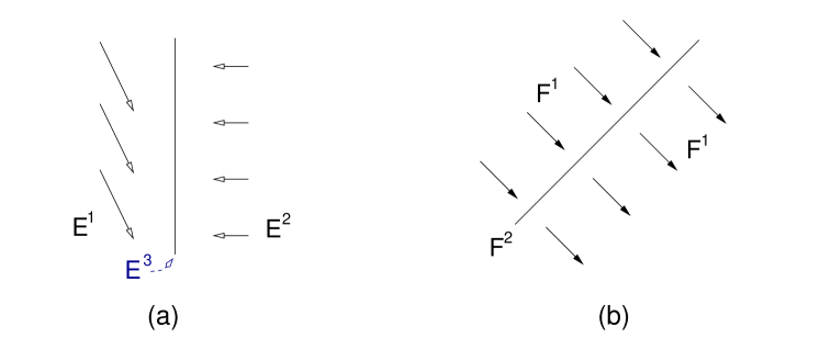
Figure 2. Integral curves for the network vector field may not be well defined (a) and may differ from those given by the Filippov conventions (b).

(1) Take event sets $E^{1}=\{(x_{1},x_{2})\,|\,x_{1}\leq 0\}$, $E^{2}={}^{2}\smallsetminus E^{1}$, and corresponding constant vector fields $\mathbf{f}^{1}=(1,-2)$, $\mathbf{f}^{2}=(-1,0)$ (see figure 2(a)). Trajectories cannot be continued, according to definition 4.15, once they meet $x_{1}=0$. One way round this problem is to define a new event set $E^{3}=\partial E^{1}$ and the sliding vector field $\mathbf{f}^{3}=\mathbf{f}^{1}+\mathbf{f}^{2}=(0,-2)$. There is then a complete integral curve through every point of ² and the corresponding semiflow $\Phi:{}^{2}\times{}_{+}\rightarrow{}^{2}$ is continuous. This approach is based on the Filippov construction [27, Chapter 2, page 50] where we take a vector field in the positive cone defined by $\mathbf{f}^{1},\mathbf{f}^{2}$ (often the unique convex combination $\lambda\mathbf{f}^{1}+(1-\lambda)\mathbf{f}^{2}$) which is tangent to $\partial E^{1}=E^{3}$).

(2) Take event sets $F^{1}=\{(x_{1},x_{2})\,|\,x_{1}\neq x_{2}\}$, $F^{2}=\{(x_{1},x_{2})\,|\,x_{1}=x_{2}\}$, and corresponding vector fields $\mathbf{f}^{1}(x_{1},x_{2})=(1,-1)$, $\mathbf{f}^{2}(x_{1},x_{2})=(0,0)$ (see figure 2(b) and note that the event $F^{2}$ models a collision, after which dynamics stops). Integral curves are defined for all initial conditions in ² but the semiflow $\Phi:{}^{2}\times{}_{+}\rightarrow{}^{2}$ will not be continuous on $F^{2}$. Here the Filippov construction gives the wrong network solution – the diagonal $F^{2}$ is regarded as a removable singularity.

We discuss the relationship between asynchronous networks and Filippov systems further in section 5.1.3; see also [12]. $\diamondsuit$

Definition 4.18.

The asynchronous network $\mathfrak{N}$ is proper if for all $\mathbf{X}\in\mathbf{M}$, the maximal integral curve through $\mathbf{X}$ is complete: $\boldsymbol{\phi}_{\mathbf{X}}:[0,\infty)\rightarrow\mathbf{M}$.

Remarks 4.19.

(1) If $\mathfrak{N}$ is proper, network dynamics is given by a semiflow $\Phi:\mathbf{M}\times{}_{+}\rightarrow\mathbf{M}$. Although $\Phi(\mathbf{X},t)$ will be continuous as a function of $t\in{}_{+}$, it need not be continuous as a function of $\mathbf{X}\in\mathbf{M}$ (see examples 4.17(2)).
(2) In many cases of interest, some of the node phase spaces $M_{i}$ may be open domains in ⁿ with with $\partial M_{i}\neq\emptyset$. Here there is the possibility that trajectories may exit $\mathbf{M}$: if $\boldsymbol{\phi}=(\boldsymbol{\phi}_{1},\dotsc,\boldsymbol{\phi}_{k})$ is a trajectory, there may exist $i\in\mathbf{k}$ and a smallest $s>0$ such that $\boldsymbol{\phi}_{i}(s)\stackrel{{\scriptstyle\mathrm{def}}}{{=}}\lim_{t\rightarrow s_{-}}\boldsymbol{\phi}_{i}(t)\in\partial M_{i}$. The maximal domain for $\boldsymbol{\phi}$ is necessarily $[0,s)$. Under additional hypotheses, it may be possible to extend $\boldsymbol{\phi}$ to a complete trajectory by setting $\mathbf{F}_{j}\equiv 0$ on ${}^{n}\smallsetminus M_{j}$, $j\in\mathbf{k}$ (the $j$th component of $\boldsymbol{\phi}$ is stopped when it meets the boundary of $M_{j}$). In this way, we can regard $\mathfrak{N}$ as proper. We develop this point of view further in part II [13].

Event sets are typically defined by analytic and algebraic conditions that reflect logical conditions on the underlying dynamics.

Definition 4.20.

Let $\mathfrak{N}$ be an asynchronous network. The event structure $\{E^{\alpha}\,|\,\alpha\in\mathcal{A}\}$ of $\mathfrak{N}$ is regular if the event sets $E^{\alpha}$ are all semianalytic subsets of $\mathbf{M}$.

Remark 4.21.

For the examples in this paper, event sets will typically be semialgebraic – defined by polynomial equalities and inequalities.

Definition 4.22.

An asynchronous network $\mathfrak{N}$ is amenable if

1. The event structure $\{E^{\alpha}\,|\,\alpha\in\mathcal{A}\}$ is regular.

2. If $\mathbf{X}\in E^{\alpha}$, $\alpha\in\mathcal{A}$, there exists a maximal $t(\mathbf{X})\in(0,\infty]$ such that the integral curve $\boldsymbol{\phi}_{\mathbf{X}}$ through $\mathbf{X}$ is defined on $[0,t(\mathbf{X}))$ and

   $$\boldsymbol{\phi}_{\mathbf{X}}(t)\in E^{\alpha},\;\;t\in[0,t(\mathbf{X})).$$

3. Either $M_{i}$ is compact without boundary or $M_{i}={}^{n_{i}}$ and vector fields have at most linear growth on $M_{i}$: $\exists a,b>0$ such that

   $$\|\mathbf{f}_{i}^{\alpha}(\mathbf{X})\|\leq a+b\|\mathbf{X}\|,\;\mathbf{X}\in\mathbf{M},\;\alpha\in\mathcal{A}.$$

Remarks 4.23.

(1) Condition (2) of definition 4.22 suggests that the vector field $\mathbf{f}^{\alpha}$ should in some sense be tangent to $E^{\alpha}$. The issue of tangency can be made precise using the regularity assumption which implies that $E^{\alpha}$ has a locally finite stratification into submanifolds without boundary (for example, the canonical Whitney regular stratification of each event set [31, 48]). This allows us to unambiguously define tangency at points of $E^{\alpha}$ which do not lie in the boundary of strata. Care is needed at points lying in the boundary of strata and in the example below we indicate how the geometric structure of the event set can impose strong constraints on associated vector fields.
(2) If an event set is a closed submanifold without boundary, it follows from definition 4.22(2) that any trajectory that meets the event set will never leave the event set.
(3) In part II we extend definition 4.22(3) to allow for trajectories to exit the domain and stop (see remark 4.19(2)).
(4) We may extend the definition of amenability to include asynchronous networks which are equivalent to an amenable network.

Examples 4.24.

Take $k=2$, $M_{1}=M_{2}=\real$.
(1) As event sets take the semialgebraic subsets of ² defined by

$$E^{1}=\{(x,0)\,|\,x<0\},\;E^{2}=\{(0,y)\,|\,y>0\},\;E^{0}={}^{2}\smallsetminus\bigcup_{i=1}^{2}E^{i}.$$

The event sets are neither open nor closed. We define associated vector fields $\mathbf{f}^{j}$, $j\in{\mathbf{2}}^{\bullet}$, on ² by

$$f^{1}(x,y)=(1,0),\;f^{2}(x,y)=(0,-1),\;f^{0}=f^{1}+f^{2}.$$

It is a simple exercise to verify that the network is amenable and proper but that the associated semiflow $\Phi:{}^{2}\times{}_{+}\rightarrow{}^{2}$ is not continuous along $E^{1}$ or $E^{2}$ (it is continuous at $(0,0)$).

(2) Suppose that the event set $E^{1}$ is the cusp defined by $\{(x,y)\in{}^{2}\,|\,x\neq 0,\;y^{2}=x^{3}\}$ and $E^{2}={}^{2}\smallsetminus E^{1}$. In this case any smooth ($C^{1}$ suffices) vector field on ² which is tangent to $E^{1}$ must vanish at $\{(0,0)\}$ (an example of such a vector field is $(2ax,3ay)$, $a\in\real$). If we require amenability, then all trajectories which meet $E^{1}$ will never leave $E^{1}$. $\diamondsuit$

Proposition 4.25.

An amenable asynchronous network is proper.

Proof.

We give details for the case when $\mathbf{M}$ is compact. Fix $\mathbf{X}\in\mathbf{M}$. Suppose that $\boldsymbol{\phi}_{i}:[0,s_{i})\rightarrow\mathbf{M}$ are forward trajectories for $\mathbf{F}$ through $\mathbf{X}$, $i\in\mathbf{2}$. Using uniqueness of solutions of differential equations and definition 4.22(2), it is easy to see that $\boldsymbol{\phi}_{1}=\boldsymbol{\phi}_{2}$ on $[0,s_{1})\cap[0,s_{2})$. It follows that if we define

$$T=\sup\left\{t\,|\,\text{there is a trajectory $\boldsymbol{\psi}:[0,t)\rightarrow\mathbf{M}$ through $\mathbf{X}$}\right\}$$

then we have a unique trajectory $\boldsymbol{\phi}:[0,T)\rightarrow\mathbf{M}$ through $\mathbf{X}$. If $T=\infty$, we are done. But if $T<\infty$, then we can extend $\boldsymbol{\phi}$ to $[0,T]$ by $\boldsymbol{\phi}(T)=\lim_{t\rightarrow T-}\boldsymbol{\phi}(t)$ (remarks 4.23(3)). If $\boldsymbol{\phi}(T)\in E^{\alpha}$ then by definition 4.22(2), $\boldsymbol{\phi}$ extends to $[0,T+t(\boldsymbol{\phi}(T)))$, where $t(\boldsymbol{\phi}(T))>0$. This contradicts the maximality of $T$ and so $T=\infty$. ∎

Remarks 4.26.

(1) Proposition 4.25 says nothing about the number of changes in the event map that occur along a trajectory. Without further conditions, there may be a countable infinity of changes with countably many accumulation points (see definition 4.15 and note the analogy with Zeno-like behaviour [11]).
(2) As shown in examples 4.24(1), the semiflow given by proposition 4.25 need not be continuous (as a function of $(\mathbf{X},t)$).
(3) Amenability is sufficient but not necessary for properness.

4.8. Semiflows for amenable asynchronous networks

Assume $\mathfrak{N}$ is an amenable asynchronous network with network vector field $\mathbf{F}$. For each $\alpha\in\mathcal{A}$, denote the flow of $\mathbf{f}^{\alpha}$ by $\Phi^{\alpha}$.

Let $\mathbf{X}\in\mathbf{M}$ and $\boldsymbol{\phi}:{}_{+}\rightarrow\mathbf{M}$ be the maximal integral curve through $\mathbf{X}$ for $\mathbf{F}$. If follows from the definition of integral curve and amenability that there is a countable closed subset $D=D(\mathbf{X})$ of ${}_{+}\cup\{\infty\}$ such that for each $u\in D$, there exist unique $\alpha\in\mathcal{A}$, $v=v(u)\in D$ such that

$$(u,v)\cap D=\emptyset,\;\mathcal{E}(v)\neq\alpha,\;\boldsymbol{\phi}([u,v))\subset E^{\alpha}.$$

(For $\mathcal{E}(u)=\alpha$ we need amenability.)

Proposition 4.27.

Let $\mathfrak{N}$ be an amenable asynchronous network. Suppose that for all $\mathbf{X}\in\mathbf{M}$, $D(\mathbf{X})$ is finite and set $D(\mathbf{X})=\{t^{\mathbf{X}}_{j}\,|\,0=t^{\mathbf{X}}_{0}<t^{\mathbf{X}}_{1}<\dotsc<t^{\mathbf{X}}_{N}<t^{\infty}_{N+1}=\infty\}$, $\alpha^{\mathbf{X}}_{j}=\mathcal{E}(\boldsymbol{\phi}(t^{\mathbf{X}}_{j}))$, $j\in{\mathbf{N}}^{\bullet}$. The semiflow $\Phi:\mathbf{M}\times{}_{+}\rightarrow\mathbf{M}$ for $\mathbf{F}$ is given in terms of the flows $\Phi^{\alpha}$ by

$$\Phi_{\mathbf{X}}(t)=\Phi^{\alpha_{p}^{\mathbf{X}}}(\cdots\Phi^{\alpha_{1}^{\mathbf{X}}}(\Phi^{\alpha^{\mathbf{X}}_{0}}(\mathbf{X},t^{\mathbf{X}}_{1}),t^{\mathbf{X}}_{2}-t^{\mathbf{X}}_{1})\cdots,t-t^{\mathbf{X}}_{p}),$$

where $t\in[t^{\mathbf{X}}_{p},t^{\mathbf{X}}_{p+1})$, $p\in{\mathbf{N}}^{\bullet}$.

Proof.

For $t\in[t^{\mathbf{X}}_{p},t^{\mathbf{X}}_{p+1})$, $\Phi^{\alpha_{p}^{\mathbf{X}}}(\mathbf{X}_{p},t)$ is the solution to $\mathbf{X}^{\prime}(t)=\mathbf{f}^{\alpha_{p}^{\mathbf{X}}}(\mathbf{X})$ with initial condition $\mathbf{X}_{p}=\Phi_{\mathbf{X}}(t_{p}^{\mathbf{X}})$. ∎

4.9. Asynchronous networks with additive input structure

A natural source of asynchronous networks comes from synchronous networks with additive input structure. The event map can be either state dependent (with constraints) or stochastic (see the following section).

Fix a $k$ node synchronous network $\mathcal{N}$ with additive input structure and network vector field $\mathbf{f}=(f_{1},\dotsc,f_{k})$ given by.

(4) $$f_{i}(\mathbf{x}_{i};\mathbf{x}_{j_{1}},\dotsc,\mathbf{x}_{j_{e_{i}}})=F_{i}(\mathbf{x}_{i})+\sum_{s=1}^{e_{i}}F_{ij_{s}}(\mathbf{x}_{j_{s}},\mathbf{x}_{i}),\;i\in\mathbf{k}.$$

On account of the additive input structure, it is natural to remove and later reinsert connections between nodes.

For $i\in\mathbf{k}$, let $(W_{i},\mathcal{L}_{i})$ be the constraint defined by the $0$-dimensional foliation of $W_{i}=M_{i}$. If dynamics on $N_{i}$ is constrained, then dynamics is stopped: ${\mathbf{x}}_{i}^{\prime}=0$. Let $\Gamma$ be the network graph determined by (4) with associated $0$ -$1$  matrix $\gamma\in M(k)$. Take $\mathbf{P}=(1,\dotsc,1)$ and let $\mathcal{A}\subset M_{\bullet}(k)$ be a generalized connection structure such that

1. $(0\,|\,\gamma)\in\mathcal{A}$,

2. for all $\alpha=(\alpha^{0}\,|\,\alpha^{\flat})$ the matrix $\alpha^{\flat}$ defines a subgraph of $\Gamma$, and

3. $\alpha_{i0}\in\{0,1\}$ for all $i\in\mathbf{k}$, $\alpha\in\mathcal{A}$.

For each $\alpha\in\mathcal{A}$, define the $\alpha$-admissible vector field $\mathbf{f}^{\alpha}$ by

$$f^{\alpha}_{i}(\mathbf{x}_{i};\mathbf{x}_{j_{1}},\dotsc,\mathbf{x}_{j_{e_{i}}})=(1-\alpha_{i0})\left(F_{i}(\mathbf{x}_{i})+\sum_{s=1}^{e_{i}}\alpha_{ij_{s}}F_{ij_{s}}(\mathbf{x}_{j_{s}},\mathbf{x}_{i})\right),\;i\in\mathbf{k},$$

and set $\mathcal{F}=\{\mathbf{f}^{\alpha}\,|\,\alpha\in\mathcal{A}\}$. If we choose an event map $\mathcal{E}:\mathbf{M}\to\mathcal{A}$ and take $\mathcal{F}=\left\{\mathbf{f}^{\alpha}\,|\,\alpha\in\mathcal{A}\right\}$, then $\mathfrak{N}=(\mathcal{N},\mathcal{A},\mathcal{F},\mathcal{E})$ is an asynchronous network. We refer to $\mathfrak{N}$ as an asynchronous network with additive input structure.

For $\alpha\in\mathcal{A}$, $i\in\mathbf{k}$, let $J(i,\alpha)=\{j\,|\,\alpha_{ij}=1,j\in{\mathbf{k}}^{\bullet}\}$ be the dependency set of $f_{i}^{\alpha}$.

Definition 4.28.

An asynchronous network $\mathfrak{N}$ is input consistent if for any node $N_{i}$ and $\alpha,\beta\in\mathcal{A}$ with dependency sets satisfying $J(i,\alpha)=J(i,\beta)$ we have $f_{i}^{\alpha}=f_{i}^{\beta}$.

As an immediate consequence of our constructions we have

Lemma 4.29.

Asynchronous networks with additive input structure are input consistent.

In summary, if $\mathfrak{N}$ is an asynchronous network with additive input structure all the admissible vector fields are derived from the network vector field of a synchronous network.

4.10. Local clocks on an asynchronous network

In this section we describe local clocks on an asynchronous network. We give only brief details sufficient for the examples we give later (the general set up appears in [14]). Roughly speaking, a local clock will be associated to a set of nodes, or connections, and may be thought of thought of as a stopwatch with time $\tau\in{}_{+}$. In particular, the local clock will run intermittently and switching between on and off states will be determined by thresholds.

Fix a finite set of nodes $\mathcal{N}=\{N_{0},N_{1},\dotsc,N_{k}\}$ with associated phase spaces $M_{i}$, $i\in\mathbf{k}$, a generalized connection structure $\mathcal{A}\subset M_{\bullet}(k)$ and a constraint structure $\mathbf{C}$. Local clocks will be defined in terms of strongly connected components of elements of $\mathcal{A}$.

Suppose that $\alpha\in\mathcal{A}$ and let $\beta,\gamma$ be distinct strongly connected components of $\alpha$ with respective node sets $A\subset\mathbf{k}$, $B\subset{\mathbf{k}}^{\bullet}$. A local time $\tau_{\beta,\gamma}\in{}_{+}$ will be defined on $\beta$ (or the nodes $A$) if there exists a connection $N_{j}\rightarrow N_{i}$, $j\in B$, $i\in A$.

Examples 4.30.

(1) The constraining node $N_{0}$ is always a strongly connected component of $\alpha$. If $\alpha=N_{0}\rightarrow N_{i}$, then we may take $\beta=\{N_{i}\}$, $\gamma=\{N_{0}\}$ and define the local time $\tau_{i}$ on $N_{i}$.
(2) If $\alpha=N_{0}\rightarrow N_{i}\leftrightarrow N_{j}\leftarrow N_{0}$, then we may take $\beta=N_{i}\leftrightarrow N_{j}$, $\gamma=\{N_{0}\}$ and obtain the local time $\tau_{\beta}=\tau_{ij}$ defined on $N_{i},N_{j}$ (or $N_{i}\leftrightarrow N_{j}$). $\diamondsuit$

Choose a set $\tau_{1},\dotsc,\tau_{s}$ of local times and set

$$\mathcal{T}={}_{+}^{s}=\{\boldsymbol{\tau}=(\tau_{1},\dotsc,\tau_{s})\,|\,\tau_{1},\dotsc,\tau_{s}\in{}_{+}\}.$$

We extend the phase space of $\mathcal{N}$ to $\mathcal{M}=\mathbf{M}\times\mathcal{T}$. Given $\alpha\in\mathcal{A}$, an $\alpha$-admissible vector field $\mathbf{f}^{\alpha}$ on $\mathcal{M}$ will be a smooth vector field of the form

$$\mathbf{f}^{\alpha}(\mathbf{X},\boldsymbol{\tau})=(f_{1}^{\alpha}(\mathbf{X},\boldsymbol{\tau}),\dotsc,f_{k}^{\alpha}(\mathbf{X},\boldsymbol{\tau}),h_{1},\dotsc,h_{s}),$$

where $h_{1},\dotsc,h_{s}\in\{0,1\}$ are constant vector fields.

Just as before, we define an $\mathcal{A}$-structure $\mathcal{F}$, an event map $\mathcal{E}:\mathcal{M}\rightarrow\mathcal{A}$ and associated asynchronous network $(\mathcal{N},\mathcal{A},\mathcal{F},\mathcal{E})$. Our previous definitions and results continue to apply.

Example 4.31.

Suppose $k=1$, $\mathcal{N}=\{N_{0},N_{1}\}$, and $M_{1}=\real$. Choose a smooth vector field $f:\real\rightarrow\real$ such that $1\geq f(x)>0$ for all $x\in\real$. Define $\mathcal{A}=\{{\boldsymbol{\emptyset}},\alpha=N_{0}\rightarrow N_{1}\}$. Define the local time $\tau\in{}_{+}$ associated to $\alpha$. Set $\mathcal{M}=\real\times{}_{+}$. Define $\mathcal{F}=\{\mathbf{f}^{\boldsymbol{\emptyset}},\mathbf{f}^{\alpha}\}$ by

$$\mathbf{f}^{{\boldsymbol{\emptyset}}}(x,\tau)=(f(x),0),\;\mathbf{f}^{\alpha}(x,\tau)=(0,1),\;(x,\tau)\in\mathcal{M}.$$

Fix $T>0$ and define the event map $\mathcal{E}:\mathcal{M}\rightarrow\mathcal{A}$ by

$$\mathcal{E}(x,\tau) = {\boldsymbol{\emptyset}},\;\text{if }x\neq 0\;\text{or }\tau\geq T$$

$$= \alpha,\;\text{if }x=0\;\text{and }\tau<T$$

The asynchronous network $(\mathcal{N},\mathcal{A},\mathcal{F},\mathcal{E})$ is amenable. If we initialize at $(x_{0},0)$, $x_{0}<0$, then the system evolves until $x=0$, stops for local time $T$ seconds and then restarts. In practice, the local clock is reset to zero after the system restarts. $\diamondsuit$

4.11. Stochastic event processes and asynchronous networks

Given node set $\mathcal{N}$, constraint structure $\mathbf{C}$, generalized connection structure $\mathcal{A}$ and $\mathcal{A}$-structure $\mathcal{F}$, an event process is a state dependent stochastic process $\mathcal{E}_{(t,\mathbf{X})}$ taking values in $\mathcal{A}$.

Definition 4.32.

(Notation as above.) A stochastic asynchronous network $\mathfrak{N}$ is a quadruple $(\mathcal{N},\mathcal{A},\mathcal{F},\mathcal{E})$, where $\mathcal{E}=\mathcal{E}_{(t,\mathbf{X})}$ is an event process.

In the most general case there are no restrictions on the process $\mathcal{E}_{(t,\mathbf{X})}$: there may be (stochastic) dependence on time $t\in\mathbb{R}^{+}$, pure space dependence ($\mathcal{E}_{(t,\mathbf{X})}=\mathcal{E}(\mathbf{X})$), or both. If $\mathcal{E}_{(t,\mathbf{X})}$ is independent of time, then the event process reduces to an event map $\mathcal{E}:\mathbf{M}\rightarrow\mathcal{A}$. If $\mathcal{E}_{(t,\mathbf{X})}$ is independent of $\mathbf{X}$, then under mild conditions on $\mathcal{E}$, such as assuming $\mathcal{E}$ is Poisson, integral curves on the stochastic asynchronous network $(\mathcal{N},\mathcal{A},\mathcal{F},\mathcal{E}_{t})$ will be almost surely piecewise smooth.

We discuss stochastic asynchronous networks in more detail in [14]. We give one simple example here related to additive input structure.

Example 4.33.

We follow the assumptions and notational conventions of section 4.9 and assume given a synchronous network with additive input structure and dynamics given by (4). Let $\mathcal{A}$ be a generalized connection structure and $\mathcal{E}$ be a time dependent event process taking values in $\mathcal{A}$. Assume $\mathbf{M}$ is compact and the set of times $t_{0}<t_{1}<\dotsc$ where the connection structure changes has Poisson statistics. The stochastic asynchronous network $(\mathcal{N},\mathcal{A},\mathcal{F},\mathcal{E})$ is an example of a stochastic asynchronous networks with additive input structure. Almost surely, trajectories will be piecewise smooth and defined for all positive time. $\diamondsuit$

5. Model examples of asynchronous networks

In this section, we describe two asynchronous networks using the formalism and ideas developed in the previous section. We refer also to [14], for the detailed description of an asynchronous network modelling spiking neurons, adaptivity and learning (STDP).

5.1. A transport example: train dynamics

We use a simple transport example – a single track line with a passing loop – to illustrate characteristic features of asynchronous networks in a setting requiring minimal structure and background knowledge.

Consider two trains $\mathfrak{T}_{1},\mathfrak{T}_{2}$ travelling in opposite directions along a single track railway line; see figure 3. We assume no central control and no communication between train drivers unless both trains are in the passing loop.

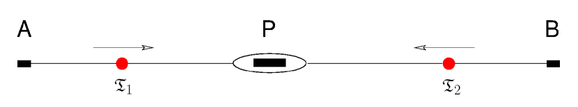
Figure 3. Two trains on a single track railway line with a passing loop and stations.

Take as phase spaces for the trains the closed interval $I=[-a,b]$, where $a,b>0$. Suppose the end points of $I$ correspond to the stations $A$ (at $-a$) and $B$ (at $b$) and that the passing loop is at $0\in I$. Assume that the passing loop is associated with a third station $P$.

The position of train $\mathfrak{T}_{i}$ at time $t\geq 0$ will be denoted by $x_{i}(t)\in I$, $i\in\mathbf{2}$. Suppose that $x_{1}(0)=-a$, $x_{2}(0)=b$. Assume that, outside of the stations $A,B,P$, the velocity of the trains is given by smooth vector fields $V_{1},V_{2}:I\rightarrow\real$ satisfying

$$V_{1}(x)>0>V_{2}(x),\;x\in I.$$

That is, $\mathfrak{T}_{1}$ is moving to the right and $\mathfrak{T}_{2}$ to the left. In order to pass each other, the trains must enter the passing loop and stop at $P$.

Fix thresholds $S,S_{1},S_{2},T_{1},T_{2}\in{}_{+}$. Train $\mathfrak{T}_{i}$ will depart at time $T_{i}$, $i\in\mathbf{2}$. We require that trains have to be together in station $P$ for time $S$ and, additionally, the train $\mathfrak{T}_{i}$ must be in the station for time $S_{i}$, $i\in\mathbf{2}$ (this is an additional condition on $\mathfrak{T}_{i}$ only if $S_{i}>S$). The trains can move out of the station when these thresholds are met. Note that the trains will not generally leave the station at the same time if $S_{1}>S$ or $S_{2}>S$. We model train dynamics by an asynchronous network.

First we discuss connection structures. Associate the node $N_{i}$ with train $\mathfrak{T}_{i}$, $i\in\mathbf{2}$. Train $\mathfrak{T}_{i}$ will be stopped at $P$ only if there is a connection $\alpha_{i}=N_{0}\rightarrow N_{i}$, $i\in\mathbf{2}$. We only allow communication between trains when both trains are stopped at $P$. In this case, the connection structure will be $\beta=N_{0}\rightarrow N_{1}\leftrightarrow N_{2}\leftarrow N_{2}$. If either train is not stopped at $P$, there is no connection between the trains.

As the drivers of the trains cannot communicate (unless both trains are in the station $P$) and there is no central control, the times associated with the thresholds $S_{1},S_{2}$ will be local times. Specifically, when train $\mathfrak{T}_{i}$ stops at $P$, the driver’s stopwatch will be started. This will be a local time $\tau_{i}$ for $\mathfrak{T}_{i}$ and associated to the connection $N_{0}\rightarrow N_{i}$, When both trains are stopped at $P$, we use a third local time $\tau=\tau_{12}$ associated to the connection $N_{1}\leftrightarrow N_{2}$ (alternatively, the drivers could synchronize their stopwatches but still the stopwatches may not run at the same speed).

We describe this setup using our formalism for asynchronous networks. As network phase space we take

$$\mathcal{M}=\{(\mathbf{X},\boldsymbol{\tau})=(x_{1},x_{2},\tau_{1},\tau_{2},\tau)\,|\,x_{1},x_{2}\in I,\;\tau_{1},\tau_{2},\tau\in{}_{+}\}=I^{2}\times{}_{+}^{3}.$$

We define the generalized connection structure $\mathcal{A}=\{\alpha_{1},\alpha_{2},\beta,{\boldsymbol{\emptyset}}\}$ and let $\mathcal{F}$ be the $\mathcal{A}$-structure given by

$$\mathbf{f}^{\boldsymbol{\emptyset}}(\mathbf{X},\boldsymbol{\tau}) = ((V_{1}(x_{1}),V_{2}(x_{2})),(0,0,0))$$

$$\mathbf{f}^{\alpha_{1}}(\mathbf{X},\boldsymbol{\tau}) = ((0,V_{2}(x_{2})),(1,0,0))$$

$$\mathbf{f}^{\alpha_{2}}(\mathbf{X},\boldsymbol{\tau}) = ((V_{1}(x_{1}),0),(0,1,0))$$

$$\mathbf{f}^{\beta}(\mathbf{X},\boldsymbol{\tau}) = ((0,0),(1,1,1))$$

We define the event map $\mathcal{E}:\mathcal{M}\rightarrow\mathcal{A}$ by

$${\small\mathcal{E}(\mathbf{X},\boldsymbol{\tau})=\begin{cases}\alpha_{1}&\text{if }(x_{1}=0,x_{2}>0)\vee((x_{1}=0,x_{2}\leq 0)\wedge(\tau_{1}<S_{1}))\\ \alpha_{2}&\text{if }(x_{2}=0,x_{1}<0)\vee((x_{2}=0,x_{1}\geq 0)\wedge(\tau_{2}<S_{2}))\\ \beta&\text{if }(x_{1}=x_{2}=0)\wedge((\tau<S)\vee((\tau_{1}<S_{1})\wedge(\tau_{2}<S_{2})))\\ {\boldsymbol{\emptyset}}&\text{otherwise}.\end{cases}}\normalsize$$

Here we have used the logical connectives $\vee$ for or and $\wedge$ for and. Dynamics on the asynchronous network $\mathfrak{N}=(\mathcal{N},\mathcal{A},\mathcal{F},\mathcal{E})$ is given by the vector field $\mathbf{F}(\mathbf{X})=\mathbf{f}^{\mathcal{E}(\mathbf{X})}(\mathbf{X})$. Provided that we initialize so that $x_{1}(0)<0<x_{2}(0)$, $\tau_{1}(0)=\tau_{2}(0)=\tau(0)=0$, it is easy to see that $\mathfrak{N}$ is amenable.

5.1.1. Initialization, termination and function

The network $\mathfrak{N}$ has a function: each train has to traverse the line to reach the opposite station. Thus we can regard $\mathfrak{N}$ as a functional asynchronous network. Formally, define initialization and termination sets by $\mathbb{I}_{1}=\{-a\}$, $\mathbb{I}_{2}=\{b\}$ and $\mathbb{F}_{1}=\{b\}$, $\mathbb{F}_{2}=\{-a\}$ respectively. We call $\mathbb{I}=\mathbb{I}_{1}\times\mathbb{I}_{2}$ and $\mathbb{F}=\mathbb{F}_{1}\times\mathbb{F}_{2}$ the initialization and termination sets for $\mathfrak{N}$. The function of the network is to get from $\mathbb{I}$ to $\mathbb{F}$ in finite time.

Typically, the thresholds $S,S_{1},S_{2},T_{1},T_{2}\in{}_{+}$ will be chosen stochastically. For example, the starting times $T_{1},T_{2}$ according to an exponential distribution. If we initialize at $(-a,T_{1}),(b,T_{2})$, and take $\tau_{1}(0)=\tau_{2}(0)=\tau(0)=0$, it is easy to verify that solutions will be defined and continuous for all positive time under the assumption that a train stops when it reaches its termination set.

5.1.2. Adding dynamics

The trains only “interact” when both are stopped at $P$. We now add a non-trivial dynamic interaction when the trains are stopped at $P$. To this end, we additionally require that

1. The drivers are running oscillators of approximately the same frequency (randomly initialized at the start of the trip).

2. When both trains are at $P$, the oscillators are cross-coupled allowing for eventual approximate frequency synchronization.

3. The trains cannot restart until the oscillators have phase synchronized to within $\varepsilon$, where $0<\varepsilon<0.5$.

For example, fix $\omega_{1},\omega_{2}\in\real$ and define $H(\theta)=k\sin 2\pi\theta$, $\theta\in\mathbb{T}$, where $k>0$. Take as network phase space $\mathcal{M}^{*}=\mathcal{M}\times\mathbb{T}^{2}$. Define vector fields $\mathbf{h}^{\boldsymbol{\emptyset}}=\mathbf{h}^{\alpha_{1}}=\mathbf{h}^{\alpha_{2}}$ and $\mathbf{h}^{\beta}$ on $\mathcal{M}^{*}$ by

$$\mathbf{h}^{\boldsymbol{\emptyset}}(\mathbf{X},\boldsymbol{\tau},\theta_{1},\theta_{2}) = (\mathbf{0},\mathbf{0},\omega_{1},\omega_{2})$$

$$\mathbf{h}^{\beta}(\mathbf{X},\boldsymbol{\tau},\theta_{1},\theta_{2}) = (\mathbf{0},\mathbf{0},\omega_{1}+H(\theta_{2}-\theta_{1}),\omega_{2}+H(\theta_{1}-\theta_{2}))$$

Define a new $\mathcal{A}$-structure $\mathcal{F}^{*}$ by

$$\mathbf{g}^{\boldsymbol{\emptyset}}=\mathbf{f}^{\boldsymbol{\emptyset}}+\mathbf{h}^{\boldsymbol{\emptyset}},\;\mathbf{g}^{\alpha_{1}}=\mathbf{f}^{\alpha_{1}}+\mathbf{h}^{\alpha_{1}},\;\mathbf{g}^{\alpha_{2}}=\mathbf{f}^{\alpha_{2}}+\mathbf{h}^{\alpha_{2}},\;\mathbf{g}^{\beta}=\mathbf{f}^{\beta}+\mathbf{h}^{\beta},$$

where $\mathbf{f}^{\boldsymbol{\emptyset}},\mathbf{f}^{\alpha_{1}},\mathbf{f}^{\alpha_{2}},\mathbf{f}^{\beta}\in\mathcal{F}$ do not depend on $(\theta_{1},\theta_{2})\in\mathbb{T}^{2}$. Modify the event map $\mathcal{E}$ by requiring that $\mathcal{E}(\mathbf{X},\boldsymbol{\tau},\theta_{1},\theta_{2})=\beta$ iff

$$(x_{1}=x_{2}=0)\wedge((\tau<S)\vee(|\theta_{1}-\theta_{2}|>\varepsilon)\vee((\tau_{1}<S_{1})\wedge(\tau_{2}<S_{2})))$$

In this case, for almost all initializations, the oscillators will eventually phase synchronize to within $\varepsilon$ provided that $\sin^{-1}(|\omega_{1}-\omega_{2}|/2k)<2\pi\varepsilon$. In particular, if $\omega_{1}=\omega_{2}$, the oscillators will synchronize unless $|\theta_{1}(0)-\theta_{2}(0)|=0.5$.

5.1.3. Relations with Filippov systems

Assume all the thresholds of our model are zero. Note that if $S=S_{1}=S_{2}=0$, then there is no need for local clocks and we may model by the asynchronous network $\mathfrak{N}^{*}=(\mathcal{N},\mathcal{A}^{*},\mathcal{F}^{*},\mathcal{E}^{*})$, where $\mathcal{A}^{*}=\{\alpha_{1},\alpha_{2},{\boldsymbol{\emptyset}}\}$, $\mathcal{F}^{*}=\{\mathbf{f}^{\boldsymbol{\emptyset}},\mathbf{f}^{\alpha_{1}},\mathbf{f}^{\alpha_{2}}\}$, where $\mathbf{f}^{\boldsymbol{\emptyset}}(\mathbf{X})=(V_{1}(x_{1}),V_{2}(x_{2}))$, $\mathbf{f}^{\alpha_{1}}(\mathbf{X})=(0,V_{2}(x_{2}))$, $\mathbf{f}^{\alpha_{2}}(\mathbf{X})=(V_{1}(x_{1}),0)$, and the event map $\mathcal{E}^{*}$ is defined by

$$\mathcal{E}^{*}(\mathbf{X})=\begin{cases}\alpha_{1}&\text{if }x_{1}=0,x_{2}>0\\ \alpha_{2}&\text{if }x_{2}=0,x_{1}<0\\ {\boldsymbol{\emptyset}}&\text{otherwise}.\end{cases}$$

We show dynamics for $\mathfrak{N}^{*}$ in figure 4 under the initialization assumption that $x_{1}(0)\leq 0\leq x_{2}(0)$.

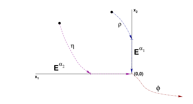
Figure 4. Dynamics on a one track line with passing loop.

Referring to the figure, trajectory $\eta$ corresponds to train $\mathfrak{T}_{2}$ reaching $P$ first and restarting only when $\mathfrak{T}_{1}$ reaches $P$. Train $\mathfrak{T}_{1}$ reaches $P$ first for the trajectory $\nu$. Regardless of which train reaches $P$ first, the ‘exit trajectory’ $\phi$ is always the same and so there is a reduction to 1-dimensional dynamics. If both trains arrive simultaneously at $P$, neither stops.

Figure 5. Dynamics for the Filippov system. Trajectories $\eta$ and $\phi$ are unchanged; trajectories $\kappa$ and $\xi$ correspond to one train reversing after the other train enters the passing loop and are artifacts of the Filippov representation.

The dynamics shown in figure 4 is suggestive of a Filippov system [27, 11] and it is natural to ask whether there are connections between asynchronous network and Filippov systems. Set ${}^{2}_{\circ}=\{(x_{1},x_{2})\,|\,x_{1}x_{2}\leq 0\}$ and observe that dynamics on $\mathfrak{N}^{*}$ is given by a continuous semiflow $\Phi^{*}:{}^{2}_{\circ}\times{}_{+}\rightarrow{}_{\circ}^{2}$. We define a Filippov system on ², with continuous semiflow $\Phi:{}^{2}\times{}_{+}\rightarrow{}^{2}$, such that $\Phi=\Phi^{*}$ on ${}^{2}_{\circ}$. To this end we let $Q_{ij}$, $i,j\in\{+,-\}$ denote the closed quadrants of ² (so $Q_{+-}=\{(x_{1},x_{2})\,|\,x_{1}\geq 0,x_{2}\leq 0\}$, etc) and define smooth vector fields on each quadrant by

$$\mathbf{V}_{++}(x_{1},x_{2}) = (-V(x_{1}),V_{2}(x_{2})),\;(x_{1},x_{2})\in Q_{++}$$

$$\mathbf{V}_{+-}(x_{1},x_{2}) = (V(x_{1}),V_{2}(x_{2})),\;(x_{1},x_{2})\in Q_{+-}$$

$$\mathbf{V}_{--}(x_{1},x_{2}) = (V(x_{1}),-V_{2}(x_{2})),\;(x_{1},x_{2})\in Q_{--}$$

$$\mathbf{V}_{-+}(x_{1},x_{2}) = (V(x_{1}),V_{2}(x_{2})),\;(x_{1},x_{2})\in Q_{-+}.$$

These vector fields uniquely define a smooth vector field $\mathbf{V}$ on the union of the interiors of the quadrants. We extend $\mathbf{V}$ to a piecewise smooth vector field on ${}^{2}\smallsetminus\{(0,0)\}$ using the Filippov conventions. Thus, we regard the $x_{i}$-axis as a sliding line $S^{i}$, $i\in\mathbf{2}$, and define $\mathbf{V}$ on $\partial Q_{-+}\cap\partial Q_{--}=E^{\alpha_{2}}\subset S^{1}$ to be the unique convex combination of $\mathbf{V}_{-+}$ and $\mathbf{V}_{--}$ which is tangent to $S^{1}$ (in this case $(\mathbf{V}_{-+}+\mathbf{V}_{--})/2$). Finally define $\mathbf{V}(0,0)=(V_{1}(0),V_{2}(0))$. The piecewise smooth vector field $\mathbf{V}$ has a continuous flow $\Phi:{}^{2}\times{}_{+}\rightarrow{}^{2}$ (integral curves are defined using the standard conventions of piecewise smooth dynamics – see [27]) and $\Phi|{}_{\circ}^{2}=\Phi^{*}$. Of course, the semiflow on ${}^{2}\smallsetminus{}_{\circ}^{2}$ does not have an interpretation in terms of trains on a line with a passing loop (see figure 5).

In an asynchronous network, dynamics on event sets is given explicitly rather than by the conventions used in Filippov systems. However, as we have shown, asynchronous networks can sometimes be locally represented by a Filippov system (see [12] for more details and greater generality). This relationship suggests the possibility of applying methods and results from the extensive bifurcation theory of nonsmooth systems to asynchronous networks.

5.1.4. Combining and splitting nodes

We conclude our discussion of asynchronous networks modelling transport with a brief description of processes defined by combining or splitting nodes (a dynamical version of a Petri Net [19]). We consider the simplest cases of two trains combining to form a single train or one train splitting to form two trains. We only give details for the first case but note that both situations are easily generalized and also, like much of what we have discussed above, apply naturally to production networks.

Consider node sets $\mathcal{N}^{a}=\{N_{0},N_{1},N_{2}\}$ and $\mathcal{N}^{b}=\{N_{0},N_{12}\}$, where $N_{1},N_{2},N_{12}$ have phase space and correspond to trains $\mathfrak{T}_{1},\mathfrak{T}_{2}$, $\mathfrak{T}_{12}$ respectively. We give a network formulation of the event where trains $\mathfrak{T}_{1},\mathfrak{T}_{2}$ are combined to form a single train $\mathfrak{T}_{12}$ (see figure 6).

Figure 6. Combining two trains into a single train.

Fix vector fields $V_{1},V_{2},V_{12}$ on and assume $V_{1}(x),V_{2}(x),V_{12}(x)>0$ all $x\in\real$. Define generalized connections structures

$$\mathcal{A}^{a} = \{{\boldsymbol{\emptyset}},\alpha_{1}=N_{0}\rightarrow N_{1},\alpha_{2}=N_{0}\rightarrow N_{2},\beta=N_{0}\rightarrow N_{1}\leftrightarrow N_{2}\leftarrow N_{2}\},$$

$$\mathcal{A}^{b} = \{{\boldsymbol{\emptyset}},\gamma=N_{0}\rightarrow N_{12}\}.$$

Assume a local clock with time $\tau=\tau_{12}$ that is shared between the connection $\beta\in\mathcal{A}^{a}$ and $\gamma\in\mathcal{A}^{b}$. Define network phase spaces for $\mathcal{N}^{a}$, $\mathcal{N}^{b}$ to be $\mathcal{M}^{a}={}^{2}\times{}_{+}$, $\mathcal{M}^{b}=\real\times{}_{+}$ respectively. Define the $\mathcal{A}^{a}$-structure $\mathcal{F}^{a}$ by

$$\mathbf{f}^{a,{\boldsymbol{\emptyset}}}=((V_{1},V_{2}),0),\;\mathbf{f}^{a,\alpha_{1}}=((0,V_{2}),0),\;\mathbf{f}^{a,\alpha_{2}}=(V_{1},0),\;\mathbf{f}^{a,\beta}=((0,0),1).$$

and the $\mathcal{A}^{b}$-structure $\mathcal{F}^{b}$ by $\mathbf{f}^{b,{\boldsymbol{\emptyset}}}=(V_{12},0),\;\mathbf{f}^{b,{\gamma}}=(0,1)$.

Fix thresholds $S_{2},S_{1}>0$. The threshold $S_{1}$ gives the time taken to combine $\mathfrak{T}_{1}$ and $\mathfrak{T}_{2}$, and $S_{2}$ models the time $\mathfrak{T}_{12}$ spends in the station before leaving. Initialize $\mathcal{N}^{a}$ so that $x_{1}(0),x_{2}(0)<0$ and $\tau(0)=0$. The event map $\mathcal{E}^{a}(\mathbf{X},\tau)$ is defined for $x_{1},x_{2}\leq 0$ and $\tau<S$ by

$$\mathcal{E}^{a}(\mathbf{X},\tau) = {\boldsymbol{\emptyset}},\;x_{1},x_{2}<0$$

$$= \alpha_{1},\;x_{1}=0,x_{2}<0$$

$$= \alpha_{2},\;x_{1}<0,x_{2}=0$$

$$= \beta,\;x_{1}=x_{2}=0,\tau<S_{1}$$

The event map $\mathcal{E}^{b}(x_{12},\tau)$ is defined for $x_{12}\geq 0$ and $\tau\geq S_{1}$ by

$$\mathcal{E}^{b}(x_{12},\tau) = \gamma,\;x_{12}=0,\tau<S_{1}+S_{2}$$

$$= {\boldsymbol{\emptyset}},\;\text{otherwise}$$

When $\tau=S_{1}$, we switch from network $\mathcal{N}^{a}$ to $\mathcal{N}^{b}$.

The splitting construction is similar except that we need to split the local clock for the combined train into two clocks, one for each separated train.

5.2. Power grids and microgrids

5.2.1. Power grids as asynchronous networks

We first consider an unrealistic, but simple and instructive model that shows how asynchronous and event dependent effects can naturally fit into the framework of power grids. In the following section, we describe how more realistic models are obtained, their limitations, and where we might expect asynchronous network models to be useful.

We use the simplest model [28] for power grid frequency stability that assumes generators are synchronous, loads are synchronous motors and consider the network of mechanical phase oscillators

(5) $$\theta_{j}^{\prime\prime}+\alpha_{j}\theta_{j}^{\prime}=P_{j}-\sum_{i=1}^{n}k_{ij}\sin(\theta_{i}-\theta_{j}),\;j\in\mathbf{n},$$

where $(k_{ij})$ is a a symmetric matrix, all entries positive (zero is allowed). If $\sum_{j}P_{j}=0$ the system can reach an equilibrium ($P_{j}<0$ corresponds to a load). Let $\Gamma$ be the (undirected) graph determined by the matrix of connections given by $(k_{ij})$. While the network described by (5) is not asynchronous (and the main interest lies with the stability of the equilibrium solution), the dynamics of real-world power grids are subject to factors that cannot be adequately described by a synchronous model. For integrity of transmission lines, as well as system stability, it is essential that the phase differences $|\theta_{i}-\theta_{j}|$ are bounded away from $\pi/2$. For example, we might require $|\theta_{i}-\theta_{j}|\leq T_{ij}$, where $T_{ij}\in(0,\pi/2)$ will be a threshold determining the safe operational load for the transmission line. This leads to the construction of state dependent event maps $\mathcal{E}_{ij}:\mathbb{T}^{n}\rightarrow\{\Gamma,\Gamma\smallsetminus\{i\leftrightarrow j\}\}$. If $|\theta_{i}-\theta_{j}|>T_{ij}$, then $\mathcal{E}_{ij}(\boldsymbol{\theta})=\Gamma\smallsetminus\{i\leftrightarrow j\}$ and the transmission line between nodes $i$ and $j$ is disconnected. Equation (5) is modified accordingly. Similarly, lines or generators may be disconnected because of external events – such as lightening strikes or mechanical breakdowns. These can be modelled using a stochastic event map.

As indicated above, this model is unrealistic (it is not true, for example, that typical loads are synchronous motors). In the next section, we indicate how more realistic models are obtained, their limitations, and where we might expect asychronous network models to be useful.

5.2.2. Network-reduced model for power grids

We give an overview of the network-reduced coupled phase oscillator model for power grids, largely based on Dörfler [20], and refer the reader to [53, 20] for greater generality, alternative models, and the many details we omit. Apart from describing the model, our goal is part cautionary (it is not evident that general theories of synchronous or asynchronous networks have much to contribute to stability problems involving structural change), and part comparative with the models we describe later for microgrids.

Assume a power grid with synchronous generators, DC power sources, transmission lines and various types of load. We assume a reference frequency $\omega_{R}$ for the power grid, usually $50$Hz or $60$Hz, and note that frequency synchronization is critical for the stability of the power grid: our equations will be written nominally in terms of phases $\theta_{i}(t)$ but for the models, we can always replace $\theta_{i}(t)$ by $\theta_{i}(t)-\omega_{R}t$ to get the (same) equations for phase deviations that are needed for stability theory (phase differences, but not absolute phases, matter).

Formally, assume given an undirected (connected) weighted graph $\mathcal{G}$ with node set $\mathcal{V}=\mathbf{n}$ and edge set $\mathcal{E}\subset\mathcal{V}^{2}$. Nodes will be partitioned as $\mathcal{V}=\mathcal{V}_{1}\cup\mathcal{V}_{2}\cup\mathcal{V}_{3},$ where $\mathcal{V}_{1}$ consists of synchronous generators, $\mathcal{V}_{2}$ are DC power sources, and $\mathcal{V}_{3}$ comprises various types of load (see below and note we do not consider all types of load).

Each edge $(i,j)\in\mathcal{E}$, $i\neq j$, is weighted by a non-zero admittance $Y_{ij}\in\mathbb{C}$ and corresponds to a transmission line. The imaginary part $\mathfrak{I}(Y_{ij})$ is the susceptance of transmission line and $\mathfrak{R}(Y_{ij})$ is the conductance. Typically, a high voltage AC transmission line is regarded as lossless ($\mathfrak{R}(Y_{ij})=0$) and inductive ($\mathfrak{I}(Y_{ij})>0$). We allow self-loops $i=j$, these will correspond to loads modelled as impedances to ground (nonzero “shunt admittances”).

To each node is associated a voltage phasor $V_{i}=|V_{i}|e^{\imath\theta_{i}}$ corresponding to phase $\theta_{i}$ and magnitude $|V_{i}|$ of the sinusoidal solution to the circuit equations.

For a lossless network, the power flow from node $i$ to node $j$ is given by $a_{ij}\sin(\theta_{i}-\theta_{j})$, where $a_{ij}=|V_{i}||V_{j}|\mathfrak{I}(Y_{ij})$ gives the maximal power flow (see Kundur [40, Chapter 6]).

5.2.3. Synchronous generators

We assume dynamics of synchronous generators are given by

(6) $$M_{i}\theta_{i}^{\prime\prime}+D_{i}\theta_{i}^{\prime}=P_{m,i}+\sum_{j=1}^{n}a_{ij}\sin(\theta_{j}-\theta_{i}),\;i\in\mathcal{V}_{1},$$

where $\theta_{i},\theta_{i}^{\prime}$ are generator rotor angle and frequency, $M_{i},D_{i}>0$ are inertia and damping coefficients, and $P_{m,i}$ is mechanical power input.

5.2.4. DC/AC inverters: droop controllers

Each DC source in $\mathcal{V}_{2}$ is connected to the AC grid via a DC/AC inverter following a frequency droop control law which obeys the dynamics [60]

(7) $$D_{i}\theta_{i}^{\prime}=P_{d,i}+\sum_{j=1}^{n}a_{ij}\sin(\theta_{j}-\theta_{i}),\;i\in\mathcal{V}_{2}.$$

5.2.5. Frequency dependent loads

We assume the active power demand drawn by load $i$ consists of a constant term $P_{l,i}>0$ and a frequency dependent term $D_{i}\theta_{i}^{\prime}$, $D_{i}>0$, leading to the power balance equation

(8) $$D_{i}\theta_{i}^{\prime}=-P_{l,i}+\sum_{j=1}^{n}a_{ij}\sin(\theta_{j}-\theta_{i}),\;i\in\mathcal{V}_{3,f},$$

where $\mathcal{V}_{3,f}$ is the subset of $\mathcal{V}_{3}$ consisting of frequency dependent loads. Equation (8) is of the same form as (7), and we may replace $\mathcal{V}_{2}$ by $\mathcal{V}_{2}\cup\mathcal{V}_{3,f}$ and consider the general equation

(9) $$D_{i}\theta_{i}^{\prime}=\omega_{i}+\sum_{j=1}^{n}a_{ij}\sin(\theta_{j}-\theta_{i}),\;i\in\mathcal{V}_{2},$$

where $\omega_{i}$ is positive if the node is a DC generator and negative if it is a frequency dependent load.

We can similarly allow for loads which are synchronous motors, incorporate them in $\mathcal{V}_{1}$ and consider

(10) $$M_{i}\theta_{i}^{\prime\prime}+D_{i}\theta_{i}^{\prime}=\omega_{i}+\sum_{j=1}^{n}a_{ij}\sin(\theta_{j}-\theta_{i}),\;i\in\mathcal{V}_{1},$$

where $\omega_{i}$ is positive if the node is a synchronous generator and negative if it is a synchronous motor.

5.2.6. Constant current and constant admittance loads

We assume the remaining loads each require a constant amount of current and have a shunt admittance (to ground). In this case we have a current balance equation and, through the process of Kron reduction [22], may obtain a reduced network the equations of which are

(11) $$M_{i}\theta_{i}^{\prime\prime}+D_{i}\theta_{i}^{\prime}=\tilde{\omega}_{i}+\sum_{j=1}^{n}\tilde{a}_{ij}\sin(\theta_{j}-\theta_{i}+\varphi_{ij}),\;i\in\mathcal{V}_{1},$$

(12) $$D_{i}\theta_{i}^{\prime}=\tilde{\omega}_{i}+\sum_{j=1}^{n}\tilde{a}_{ij}\sin(\theta_{j}-\theta_{i}+\varphi_{ij}),\;i\in\mathcal{V}_{2}.$$

We refer to [21] for the explicit form of the coefficients in (11,12).

The original power grid network is typically sparse with many nodes – $\mathcal{V}_{3}$ is large. The process of Kron reduction results in a much smaller network which will be all-to-all coupled provided that the graph defined by $\mathcal{V}_{3}$ is connected [22]. However, even if the original transmission lines are lossless, the phase shifts $\phi_{ij}$ will generally be non-zero and not necessarily always small (we refer to [53, §6.2 Figure 4] for data from a real power grid network). The presence of phase shifts can and does make it harder to frequency synchronize (11,12).

From the point of view of transmission line failure in a power grid, even if the removal of an edge still results in a all-to-all coupled reduced network, many of the coupling coefficients $\tilde{a}_{ij}$ will change. It is a hard problem, that goes beyond existing analytical theory for synchronous and asynchronous networks, to get good insight into whether or not a breakdown will destabilize the network (this is irrespective of phenomena like Braess’s paradox [64, 54]).

5.2.7. Microgrids

Assume given a stable power grid network, robust to “small” changes in power demand, and consider the problem of modelling a microgrid and its combination or separation from the main grid. We outline structural and logical issues to make transparent the connection with asynchronous networks and largely ignore dynamics so as to keep the model simple and our discussion short (we refer to [23, 60, 24, 16] for more details and references on microgrids and control from a large and rapidly developing literature in this area). Assume power generation in the microgrid is from DC generators (such as solar power or DC wind power) and that $\mathcal{V}_{1}=\emptyset$ (most motor loads are not synchronous). Assume the microgrid is Kron reduced.

Unlike the power grid model described above, we allow directed (one way) connections and a constraining node. Consider the simplified network $\mathcal{N}=\{N_{0},N_{B},N_{G},N_{P}\}$, where the nodes $N_{B},N_{G},N_{P}$ correspond to a large capacity battery (buffer), a DC generator, and main power grid respectively, and define subnetworks $\mathcal{N}_{M}=\{N_{B},N_{G}\}$ (microgrid) and $\mathcal{N}_{P}=\{N_{P}\}$ (main power grid).

The battery acts as reserve storage or buffer for the microgrid; in particular to maintain power in the event of intermittent loss of generated DC power or when the microgrid has been separated “islanded” from the main power grid. We suppose battery capacity $B=B(t)\in[0,B_{M}]$, where $B_{M}$ corresponds to the battery being fully charged. We suppose that the DC generator produces power $O=O(t)\in[0,O_{M}]$, where $O_{M}$ is the maximum power than can be generated.

The constraining node will play a role when the microgrid is islanded and is to be reconnected to the main power grid: either because the microgrid has insufficient power for the microgrid loads or because the microgrid has an excess of available power some of which can now be contributed to the main power grid. In either case a transition process needs to be implemented where the droop controller for the DC/AC converter needs to bring the AC output of the microgrid in precise voltage (phase, frequency and magnitude) synchronization with the state of the power grid at the connection point(s) to the microgrid. Similarly, we can constrain when the microgrid is to be islanded from the main grid so that the reduction in power contributed to the main power grid is gradual and done over an appropriate time scale so as not to destabilize the main power grid.

Leaving aside the dynamics of islanding and combining the microgrid with the main power grid, the generalized connection structures and control logic we need for management of the microgrid are complex and depend on several thresholds which may need to be time dependent – for example, if we use a time dependent model for the projected microgrid power load. If the microgrid is islanded, we work with $\mathcal{N}_{M}$ and use the generalized connection structure

$$\mathcal{A}_{M}=\{\alpha=N_{G}\rightarrow N_{B},\beta=N_{B}\rightarrow N_{G},{\boldsymbol{\emptyset}}\}.$$

The connection structure $\alpha$ corresponds to the DC generator having sufficient output to supply all power needed for the microgrid load and with a surplus which can be used to charge the battery, $\beta$ corresponds to battery and generator providing all necessary power for the microgrid, and ${\boldsymbol{\emptyset}}$ corresponds to the generator providing all needed power for the microgrid and either there is surplus power available for battery charging or the battery is fully charged. Thresholds that determine switching between these states are chosen so as to avoid “chattering” in the control system.

If the microgrid is combined with the main power grid, this can be either because battery and DC generators cannot provide sufficient power for the microgrid load or because the microgrid has surplus power which can be contributed to the main power grid or because the main power grid is stressed (possibly locally detected by frequency variation) and the battery state of the microgrid is sufficiently high to allow a temporary power contribution to the main grid. As generalized connection structure $\mathcal{A}$ we take the set of connection structures

$$N_{G}\rightarrow N_{M},\;N_{G}\rightarrow N_{M}\leftarrow N_{B},$$

$$N_{B}\rightarrow N_{G}\leftarrow N_{M},\;N_{M}\rightarrow N_{G},\;N_{M}\rightarrow N_{G}\rightarrow N_{B},$$

Each of these connection structures has a natural interpretation. For example, $N_{M}\rightarrow N_{G}\rightarrow N_{B}$ corresponds to the main power grid contributing to both the load of the microgrid and battery charging while $N_{G}\rightarrow N_{M}\leftarrow N_{B}$ means battery and DC generator are contributing power to the main power grid as well as supplying all the power for the microgrid. On the other hand, $N_{G}\rightarrow N_{M}$ means DC generated power, but not battery power, is being contributed to the main power grid.

Of course, what we have described above is highly simplified as we have taken no account of (1) multiple DC generators and batteries within a microgrid, or (2) multiple microgrids. In the latter case, we need to take care that microgrid switching does not synchronize as this could lead to large destabilizing changes in load on the main grid.

6. Products of asynchronous networks

We conclude part I with the definition of the product of asynchronous networks and give sufficient conditions for an asynchronous network to decompose as a product of two or more asynchronous networks. Although the methods we use are elementary, the study of products is illuminating as it clarifies some subtleties in both the event map and the functional structure that are not present in the theory of synchronous networks. These ideas play a central role in the proof of the modularization of dynamics theorem in part II.

6.1. Products

Given $\alpha,\beta\in M(k)$, define $\alpha\vee\beta\in M(k)$ (the join of $\alpha$ and $\beta$) by

$$(\alpha\vee\beta)_{ij}=\max\left\{\alpha_{ij},\beta_{ij}\right\},\;i,j\in\mathbf{k}$$

(the max-plus addition of tropical algebra [35]). We have $\alpha\vee{\boldsymbol{\emptyset}}=\alpha$ for all $\alpha\in M(k)$. If $\mathcal{A},\mathcal{B}\subset M(k)$ are generalized connection structures, define the generalized connection structure $\mathcal{A}\vee\mathcal{B}$ by

$$\mathcal{A}\vee\mathcal{B}=\left\{\alpha\vee\beta\,|\,\alpha\in\mathcal{A},\;\beta\in\mathcal{B}\right\}.$$

Note that ${\boldsymbol{\emptyset}}\in\mathcal{A}\vee\mathcal{B}$ if and only if ${\boldsymbol{\emptyset}}\in\mathcal{A}\cap\mathcal{B}$. Consequently, if ${\boldsymbol{\emptyset}}\in\mathcal{A}\vee\mathcal{B}$, then $\mathcal{A},\mathcal{B}\subset\mathcal{A}\vee\mathcal{B}$.

Suppose that $A$ is a nonempty subset of $\mathbf{k}$ containing $k_{A}$ elements. There is a natural embedding of $M(k_{A})$ in $M(k)$ defined by relabelling the matrices in $M(k_{A})$ according to $A$. Specifically, map the matrix $(\alpha_{ij})_{i,j\in A}\in M(k_{A})$ to the matrix $\widehat{\alpha}\in M(k)$ defined by

$$\widehat{\alpha}_{ij}=\begin{cases}\alpha_{ij}&\text{for }i,j\in A,\\ 0&\text{otherwise}.\end{cases}$$

This embedding extends to an embedding of $M_{\bullet}(k_{A})$ in $M_{\bullet}(k)$ by

$$\widehat{\alpha}_{i0}=\begin{cases}\alpha_{i0}&\text{for }i\in A,\\ 0&\text{otherwise.}\end{cases}$$

Given disjoint nonempty subsets $A,B$ of $k$, regard $M_{\bullet}(k_{A}),M_{\bullet}(k_{B})$ as embedded in $M_{\bullet}(k)$. Given $\alpha\in M_{\bullet}(k_{A})$, $\beta\in M_{\bullet}(k_{B})$, define

$$\alpha\vee\beta=\widehat{\alpha}\vee\widehat{\beta}\in M_{\bullet}(k).$$

This extends to the join $\mathcal{A}\vee\mathcal{B}$ of generalized connection structures on disjoint sets of nontrivial nodes.

Let $\mathcal{N}=\{N_{0},\dotsc,N_{k}\}$ and $A$ be a proper subset of $\mathbf{k}$. Define $\mathcal{N}^{A}=\{N_{j}\,|\,j\in{A}^{\bullet}\}$ and $\mathbf{M}_{A}=\prod_{i\in A}M_{i}$. Denote points in $\mathbf{M}_{A}$ by $\mathbf{X}_{A}$. Suppose $B=\mathbf{k}\smallsetminus A$. We have $\mathcal{N}^{A}\cap\mathcal{N}^{B}=\left\{N_{0}\right\}$ and $\mathbf{M}_{A}\times\mathbf{M}_{B}\approx\mathbf{M}$. If $\mathbf{C}^{A}$, $\mathbf{C}^{B}$ are constraint structures on $\mathcal{N}^{A}$, $\mathcal{N}^{B}$ respectively, let $\mathbf{C}=\mathbf{C}^{A}\vee\mathbf{C}^{B}$ denote the induced constraint structure on $\mathcal{N}$ – well defined since constraints depend only on nodes and $A\cap B=\emptyset$.

More generally, given disjoint node sets $\mathcal{N}^{A}=\{N_{j}\,|\,j\in{A}^{\bullet}\}$, $\mathcal{N}^{B}=\{N_{j}\,|\,j\in{B}^{\bullet}\}$, we can identify $A,B$ with complementary subsets of $\mathbf{k}$, where $k$ is the total number of elements in $A\cup B$, and then follow the conventions described above.

Definition 6.1.

(Notation and assumptions as above.) Given asynchronous networks $\mathfrak{N}^{X}=(\mathcal{N}^{X},\mathcal{A}^{X},\mathcal{F}^{X},\mathcal{E}^{X})$, $X\in\left\{A,B\right\}$, define the product $\mathfrak{N}^{A}\times\mathfrak{N}^{B}$ to be the asynchronous network $\mathfrak{N}=(\mathcal{N},\mathcal{A},\mathcal{F},\mathcal{E})$ where

1. $\mathcal{N}=\mathcal{N}^{A}\cup\mathcal{N}^{B}$,

2. $\mathbf{C}=\mathbf{C}^{A}\vee\mathbf{C}^{B}$,

3. $\mathcal{A}=\mathcal{A}^{A}\vee\mathcal{A}^{B}$,

4. $\mathcal{F}=\mathcal{F}^{A}\times\mathcal{F}^{B}=\{\mathbf{f}_{A}^{\alpha}\times\mathbf{f}_{B}^{\beta}\,|\,\alpha\in\mathcal{A}^{A},\;\beta\in\mathcal{A}^{B}\}$, and

5. $\mathcal{E}$ is defined by

   $$\mathcal{E}(\mathbf{X}_{A},\mathbf{X}_{B})=\mathcal{E}^{A}(\mathbf{X}_{A})\vee\mathcal{E}^{B}(\mathbf{X}_{B}),\;\text{for }(\mathbf{X}_{A},\mathbf{X}_{B})\in\mathbf{M}_{A}\times\mathbf{M}_{B}.$$

Remark 6.2.

If $\mathfrak{N}^{A},\mathfrak{N}^{B}$ are proper (or amenable), then so is $\mathfrak{N}^{A}\times\mathfrak{N}^{B}$.

Lemma 6.3.

(Notation of definition 6.1.) The network vector field on $\mathfrak{N}^{A}\times\mathfrak{N}^{B}$ is given by

(13) $$\mathbf{F}(\mathbf{X}_{A},\mathbf{X}_{B})=(\mathbf{f}_{A}^{\mathcal{E}^{A}(\mathbf{X}_{A})}(\mathbf{X}_{A}),\mathbf{f}_{B}^{\mathcal{E}^{B}(\mathbf{X}_{B})}(\mathbf{X}_{B})),$$

for all $(\mathbf{X}_{A},\mathbf{X}_{B})\in\mathbf{M}_{A}\times\mathbf{M}_{B}$.

Proof.

Immediate from the definitions. ∎

6.2. Decomposability

Definition 6.4.

An asynchronous network $(\mathcal{N},\mathcal{A},\mathcal{F},\mathcal{E})$ is decomposable if it can be written as a product of asynchronous networks. If the network is not decomposable, it is indecomposable.

Example 6.5.

Suppose that $\mathcal{N}$ is a synchronous network with connection structure $\alpha\in M(k)$ and $\alpha$-admissible network vector field $\mathbf{f}$ satisfying conditions (N1–3) of section 2. Since $\alpha$ encodes the dependencies of $\mathbf{f}$ it is trivial that $\mathcal{N}$ can be written as a product of two synchronous networks iff the network graph $\Gamma_{\alpha}$ is disconnected. $\diamondsuit$

Our aim to find sufficient conditions on an asynchronous network for it to be decomposable.

Definition 6.6.

The connection graph of the asynchronous network $\mathfrak{N}=(\mathcal{N},\mathcal{A},\mathcal{F},\mathcal{E})$ is the graph defined by the $0$ -$1$ matrix $\Gamma_{\mathfrak{N}}=\bigvee_{\alpha\in\mathcal{A}}\alpha^{\flat}$.

Lemma 6.7.

If an asynchronous network $\mathfrak{N}$ is decomposable, then the connection graph $\Gamma_{\mathfrak{N}}$ of $\mathfrak{N}$ has at least two connected components.

Proof.

If $\mathfrak{N}$ is decomposable, then $\mathfrak{N}=\mathfrak{N}^{A}\times\mathfrak{N}^{B}$, where $A,B$ are proper complementary subsets of $\mathbf{k}$. Since there are no connections between nodes in $\mathcal{N}^{A}$ and $\mathcal{N}^{B}$, $\Gamma_{\mathfrak{N}}$ has at least two connected components. ∎

Remark 6.8.

Lemma 6.7 gives a necessary condition for decomposability which is not sufficient. There are two issues. First, the event map encodes information about spatial dependence of node interactions that cannot be deduced from the connection graph. Second, the admissible vector fields may have dependencies that are incompatible with decomposability.

Example 6.9.

Let $k=2$, $M_{1}=M_{2}=\real$. Define connection structures $\alpha_{i}=N_{0}\rightarrow N_{i}$, $i\in\mathbf{2}$ and generalized connection structure $\mathcal{A}=\{{\boldsymbol{\emptyset}},\alpha_{1},\alpha_{2},\beta=\alpha_{1}\vee\alpha_{2}\}$. Suppose the event map is given by

$$\mathcal{E}(x_{1},x_{2})=\begin{cases}\alpha_{1},&\text{if }x_{1}<0,x_{2}=0\\ \alpha_{2},&\text{if }x_{1}=0,x_{2}>0\\ \beta,&\text{if }x_{1}=x_{2}=0,\\ {\boldsymbol{\emptyset}},&\text{otherwise}\end{cases}$$

In this case, $\mathcal{A}=\mathcal{A}^{1}\vee\mathcal{A}^{2}$, where $\mathcal{A}^{i}=\{{\boldsymbol{\emptyset}},\alpha_{i}\}$, $i\in\mathbf{2}$, and the network graph is disconnected. However, there is no way to write $\mathcal{E}(x_{1},x_{2})$ as $\mathcal{E}^{1}(x_{1})\vee\mathcal{E}^{2}(x_{2})$ as the event sets involving $x_{1}\in M_{1}$ depend nontrivially on $x_{2}\in M_{2}$. Hence the network cannot be decomposable or even equivalent to a decomposable network whatever choice we make for admissible vector fields.

Suppose instead we define the event map by

$$\tilde{\mathcal{E}}(x_{1},x_{2})=\begin{cases}\alpha_{1},&\text{if }x_{1}=0,x_{2}\neq 0\\ \alpha_{2},&\text{if }x_{2}=0,x_{1}\neq 0\\ \beta,&\text{if }x_{1}=x_{2}=0\\ {\boldsymbol{\emptyset}},&\text{otherwise}\end{cases}$$

In this case $\mathcal{A}=\mathcal{A}^{1}\vee\mathcal{A}^{2}$ and we may write $\mathcal{E}=\mathcal{E}^{1}\vee\mathcal{E}^{2}$ where $\mathcal{E}^{i}(0)=\alpha_{i}$, and $\mathcal{E}^{i}(x_{i})={\boldsymbol{\emptyset}}$, $x_{i}\neq 0$, $i\in\mathbf{2}$. Suppose that $\mathbf{f}^{\alpha_{1}}(x_{1},x_{2})=(0,v_{2})$, $\mathbf{f}^{\alpha_{2}}(x_{1},x_{2})=(v_{1},0)$, $\mathbf{f}^{\boldsymbol{\emptyset}}(x_{1},x_{2})=(v_{1},v_{2})$, where $v_{1},v_{2}\neq 0$. For the moment leave $\mathbf{f}^{\beta}$ unspecified. Define $\mathcal{F}^{i}=\{\mathbf{f}_{i}^{\boldsymbol{\emptyset}},\mathbf{f}_{i}^{\alpha_{i}}\}$, where $\mathbf{f}_{i}^{\boldsymbol{\emptyset}}(x_{i})=v_{i}$, $\mathbf{f}_{i}^{\alpha_{i}}(x_{i})=0$, $i\in\mathbf{2}$. Observe that $\mathbf{f}^{\boldsymbol{\emptyset}}=\mathbf{f}_{1}^{\boldsymbol{\emptyset}}\times\mathbf{f}_{2}^{\boldsymbol{\emptyset}}$, $\mathbf{f}^{\alpha_{1}}=\mathbf{f}_{1}^{\alpha_{1}}\times\mathbf{f}_{2}^{\boldsymbol{\emptyset}}$ and $\mathbf{f}^{\alpha_{2}}=\mathbf{f}_{1}^{\boldsymbol{\emptyset}}\times\mathbf{f}_{2}^{\alpha_{2}}$. For $(\mathcal{N},\mathcal{A},\mathcal{F},\mathcal{E})$ to be a product we additionally require $\mathbf{f}^{\beta}(x_{1},x_{2})=(\mathbf{f}_{1}^{\alpha_{1}}(x_{1}),\mathbf{f}_{2}^{\alpha_{2}}(x_{2}))=(0,0)$, all $(x_{1},x_{2})\in{}^{2}$. In particular, if $\mathbf{f}^{\beta}(0,0)\neq(0,0)$, the network $(\mathcal{N},\mathcal{A},\mathcal{F},\mathcal{E})$ is not even equivalent to a product network. However, if $\mathbf{f}^{\beta}(0,0)=(0,0)$, then the network $(\mathcal{N},\mathcal{A},\mathcal{F},\mathcal{E})$ will be equivalent to a product network if we redefine $\mathbf{f}^{\beta}$ to be $\mathbf{f}_{1}^{\alpha_{1}}\times\mathbf{f}_{2}^{\alpha_{2}}$ (this does not change the values of $\mathbf{f}^{\beta}$ on $E^{\beta}$). $\diamondsuit$

6.3. Sufficient conditions for decomposability

Let $\mathfrak{N}$ be an asynchronous network with $k$ nodes and $C$ be a proper connected component of the connection graph $\Gamma_{\mathfrak{N}}$. Identify $C$ with the nonempty subset of $\mathbf{k}$ corresponding to the labels of the nodes in the component $C$. Let $\overline{C}=\mathbf{k}\smallsetminus C$. Since $C$ is a connected component of $\Gamma_{\mathfrak{N}}$, we can write each $\alpha\in\mathcal{A}$ uniquely as $\alpha=\alpha_{C}\vee\alpha_{\overline{C}}$, where $\alpha_{C}$, $\alpha_{\overline{C}}$ are connection structures on $\mathcal{N}^{C}$ and $\mathcal{N}^{\overline{C}}$ respectively. Set $\mathcal{A}^{C}=\{\alpha_{C}\,|\,\alpha\in\mathcal{A}\}$. We have a well defined projection $\pi_{C}:\mathcal{A}\rightarrow\mathcal{A}^{C}$ defined by $\pi_{C}(\alpha)=\alpha_{C}$.

Define the event map $\mathcal{E}^{C}:\mathbf{M}_{C}\times\mathbf{M}_{\overline{C}}\to\mathcal{A}^{C}$ by

$$\mathcal{E}^{C}(\mathbf{X}_{C},\mathbf{X}_{\overline{C}})=\pi_{C}(\mathcal{E}(\mathbf{X}_{C},\mathbf{X}_{\overline{C}})).$$

Definition 6.10.

An asynchronous network $\mathfrak{N}$ is structurally decomposable if for any connected component $C$ of the connection graph $\Gamma_{\mathfrak{N}}$, the map $\mathcal{E}^{C}$ is independent of $\mathbf{X}_{\overline{C}}\in\mathbf{M}_{\overline{C}}$ (that is, $\mathcal{E}^{C}(\mathbf{X}_{C},\mathbf{X}_{\overline{C}})=\mathcal{E}^{1}(\mathbf{X}_{C})$ where $\mathcal{E}^{1}:\mathbf{M}_{C}\to\mathcal{A}^{C}$).

Remark 6.11.

Structural decomposability implies conditions on structural dependencies that will generally be different from the dependencies of the network vector field. For example, suppose a component $C$ of the connection graph contains the node $N_{1}$. If the node $N_{1}$ is stopped there may be a condition that $N_{1}$ will restart when the state of another node, say $N_{2}$, attains a certain value. Necessarily, $N_{2}$ must lie in $C$ (structural decomposability). However, there need be no connection between $N_{1}$ and $N_{2}$ unless $C$ contains exactly two nodes.

Suppose that $\mathfrak{N}$ is structurally decomposable and that $\Gamma_{\mathfrak{N}}$ has connected components $C_{1},\dotsc,C_{q}$. Set $\mathbf{M}_{\ell}=\mathbf{M}_{C_{\ell}}$, $\mathcal{A}^{\ell}=\pi_{C_{\ell}}(\mathcal{A})$, $\ell\in\mathbf{q}$. By structural decomposability we may write $\mathcal{E}(\mathbf{X})=\bigvee_{\ell\in\mathbf{q}}\mathcal{E}^{\ell}(\mathbf{X}_{\ell})$ where $\mathcal{E}^{\ell}:\mathbf{M}_{\ell}\rightarrow\mathcal{A}^{\ell}$. For $\alpha\in\mathcal{A}$, $\ell\in\mathbf{q}$, set $\alpha_{\ell}=\pi_{C_{\ell}}(\alpha)\in\mathcal{A}^{\ell}$ and $E^{\ell}_{\alpha_{\ell}}=(\mathcal{E}^{\ell})^{-1}(\alpha_{\ell})\subset\mathbf{M}_{\ell}$.

Lemma 6.12.

(Notation as above.) If $\mathfrak{N}$ is structurally decomposable and $\Gamma_{\mathfrak{N}}$ has connected components $C_{1},\dotsc,C_{q}$, then

$$E_{\alpha}=\prod_{\ell\in\mathbf{q}}E^{\ell}_{\alpha_{\ell}}\subset\prod_{\ell\in\mathbf{q}}\mathbf{M}_{\ell},\;\text{for all }\alpha\in\mathcal{A}.$$

Proof.

An immediate consequence of structural decomposability. ∎

If $C$ be a proper connected component of the connection graph $\Gamma_{\mathfrak{N}}$ of an asynchronous network $\mathfrak{N}$, then by admissibility

$$\mathbf{f}^{\alpha}=\mathbf{f}_{C}^{\alpha}\times\mathbf{f}_{\overline{C}}^{\alpha},\;\text{for all }\alpha\in\mathcal{A},$$

where $\mathbf{f}^{\alpha}_{C}:\mathbf{M}_{C}\to T\mathbf{M}_{C}$ and $\mathbf{f}^{\alpha}_{\overline{C}}:\mathbf{M}_{\overline{C}}\to T\mathbf{M}_{\overline{C}}$.

In order that $\mathfrak{N}$ be decomposable, this decomposition has to be compatible with the projections $\pi_{C}:\mathcal{A}\to\mathcal{A}^{C}$, $\pi_{\overline{C}}:\mathcal{A}\to\mathcal{A}^{\overline{C}}$. In particular, if connections in the set of nodes that are in $\overline{C}$ are added or deleted, dynamics on $\mathbf{M}_{C}$ is not affected.

Definition 6.13.

(Notation as above.) The asynchronous network $\mathfrak{N}$ is dynamically decomposable if for any connected component $C$ of $\Gamma_{\mathfrak{N}}$, we have

$$\mathbf{f}_{C}^{\alpha}=\mathbf{f}_{C}^{\beta}$$

for all $\alpha,\beta\in\mathcal{A}$ such that $\pi_{C}(\alpha)=\pi_{C}(\beta)$.

Lemma 6.14.

(Notation as above.) Input consistent asynchronous networks are dynamically decomposable. In particular, asynchronous networks with additive input structure are dynamically decomposable.

Proof.

Given $i\in\mathbf{k},\alpha\in\mathcal{A}$, let $J(i,\alpha)$ be the associated dependency set for node $N_{i}$. If $\alpha,\beta\in\mathcal{A}$ and $J(i,\alpha)=J(i,\beta)$, then $f_{i}^{\alpha}=f_{i}^{\beta}$ by input consistency. If $i\in C$, where $C$ is a connected component of the network graph $\Gamma_{\mathfrak{N}}$, then $J(i,\alpha)\cap\mathbf{k}\subset C$ for all $\alpha\in\mathcal{A}$. Hence $J(i,\alpha)=J(i,\alpha_{C}\vee\alpha_{\overline{C}})$ is independent of $\alpha_{\overline{C}}$. Input consistency implies that $f_{i}^{\alpha_{C}\vee\beta}=f_{i}^{\alpha_{C}\vee\gamma}$ for all $\beta,\gamma\in\mathcal{A}_{\overline{C}}$ which yields dynamical decomposability. ∎

We now state the main result of this section.

Theorem 6.15.

Let $\mathfrak{N}$ be a structurally and dynamically decomposable asynchronous network with connection graph $\Gamma$. If $\Gamma$ has connected components $C_{1},\dotsc,C_{q}$ then there exist indecomposable asynchronous networks $\mathfrak{N}^{1},\dotsc,\mathfrak{N}^{q}$ such that

$$\mathfrak{N}=\mathfrak{N}^{1}\times\dotsb\times\mathfrak{N}^{q}.$$

Proof.

For $\ell\in\mathbf{q}$, define $\mathcal{A}^{\ell}=\{\alpha_{\ell}\stackrel{{\scriptstyle\mathrm{def}}}{{=}}\pi_{\ell}(\alpha)\,|\,\alpha\in\mathcal{A}\}$ and $\mathcal{F}^{\ell}=\{\mathbf{f}_{\ell}^{\alpha_{\ell}}\stackrel{{\scriptstyle\mathrm{def}}}{{=}}\mathbf{f}_{C_{\ell}}^{\alpha}:\mathbf{M}_{\ell}\rightarrow T\mathbf{M}_{\ell}\,|\,\alpha\in\mathcal{A}\}$. By dynamical indecomposability we have $\mathbf{f}^{\alpha}=\prod_{\ell\in\mathbf{q}}\mathbf{f}_{\ell}^{\alpha_{\ell}}$, for all $\alpha\in\mathcal{A}$. Constraint structures are defined for individual nodes and so factorise naturally. Let $\mathcal{E}^{\ell}:\mathbf{M}_{\ell}\rightarrow\mathcal{A}^{\ell}$ be the event maps given by structural indecomposability. If we let $\mathfrak{N}^{\ell}$ be the asynchronous network $(\mathcal{N}^{\ell},\mathcal{A}^{\ell},\mathcal{F}^{\ell},\mathcal{E}^{\ell})$, where $\mathcal{N}^{\ell}=\{N_{0}\}\cup\{N_{i}\,|\,i\in C_{i}\}$, $\ell\in\mathbf{q}$, then $\mathfrak{N}=\prod_{\in\mathbf{q}}\mathfrak{N}^{i}$. ∎

Our concluding result on decomposability is an immediate consequence of lemma 6.7 and theorem 6.15.

Corollary 6.16.

A structurally and dynamically decomposable asynchronous network $\mathfrak{N}$ is decomposable if and only if its connection graph has more than one nontrivial connected component.

6.4. Factorization of asynchronous networks

Assume for this section that $\mathfrak{N}=(\mathcal{N},\mathcal{A},\mathcal{F},\mathcal{E})$ is an asynchronous network which is not necessarily structurally or dynamically indecomposable.

Definition 6.17.

The asynchronous network $\mathfrak{N}^{1}$ is a factor of $\mathfrak{N}$ if there is an asynchronous network $\mathfrak{N}^{2}$ such that $\mathfrak{N}=\mathfrak{N}^{1}\times\mathfrak{N}^{2}$.

The proof of the next lemma is immediate from the definition of a product.

Lemma 6.18.

If $\mathfrak{N}^{1}$ is a factor of $\mathfrak{N}$, then the connection graph $\Gamma_{\mathfrak{N}^{1}}$ is a union of connected components of $\Gamma_{\mathfrak{N}}$.

Remark 6.19.

If $\mathfrak{N}^{1}$ is indecomposable, the connection graph $\Gamma_{\mathfrak{N}^{1}}$ may have more than one component – unless $\mathfrak{N}$ is structurally and dynamically indecomposable (theorem 6.15).

Proposition 6.20.

Every asynchronous network $\mathfrak{N}$ has a factorization $\prod_{a\in\mathbf{q}}\mathfrak{N}^{a}$ as a product of indecomposable asynchronous networks. The factorization is unique, up to the order of factors.

Proof.

Existence is obvious. The uniqueness of factorization follows easily from lemma 6.18. ∎

Acknowledgements. CB would like to thank Marc Timme at the Max Planck Institute for Dynamics and Self-Organization for continuing hospitality. MF would like to thank the Mathematics Department at Rice University, where much of this work was done, for providing a warm and supportive working environment, and Steve Furber of Manchester University for his penetrating insights and questions. Both authors would like to acknowledge fruitful discussions with many people — too many to name individually here — whose input has proved invaluable in helping to shape these ideas.

References

- [1] N Agarwal & M Field. ‘Dynamical equivalence of networks of coupled dynamical systems I: asymmetric inputs’, Nonlinearity 23 (2010), 1245–1268.
- [2] N Agarwal & M Field. ‘Dynamical equivalence of networks of coupled dynamical systems II: general case’, Nonlinearity, 23 (2010), 1269–1289.
- [3] M Aguiar, A P S Dias, P Ashwin, & M Field. ‘Dynamics of coupled cell networks: synchrony, heteroclinic cycles and inflation’, Journal of Nonlinear Science, 21(2) (2011), 271–323.
- [4] U Alon. An Introduction to Systems Biology. Design Principles of Biological Circuits (Chapman & Hall/CRC, Boca Raton, 2007).
- [5] P W Anderson. ‘More is different’, Science 177(4047) (1972), 393–396.
- [6] D V Anosov. ‘Stability of equilibrium positions in relay systems’, Automation Remote Control 20 (1959), 135–149.
- [7] A L Barab’asi and R Albert. ‘Statistical mechanics of complex networks’, Rev. Mod Phy. 74 (2002), 47–94.
- [8] V Belykh, I Belykh, and M Hasler. ‘Connection graph stability method for synchronized coupled chaotic systems’, Physica D 195(1-2) (2004), 159–187.
- [9] I Belykh, M di Bernardo, J Kurths, & M Porfri. ‘Evolving dynamical networks’, Physica D, 267 (2014), 1–6.
- [10] M di Bernardo, C J Budd, & A R Champneys, ‘Normal form maps for grazing bifurcations inn-dimensional piecewise-smooth dynamical systems’, Physica D 160 (2001), 222-254.
- [11] M di Bernardo, C J Budd, A R Champneys, & P Kowalczyk. Piecewise-smooth Dynamical Systems (Springer, Applied Mathematical Science 163, London, 2008).
- [12] C Bick. ‘Local representation of asynchronous networks by Filippov systems’, in preparation.
- [13] C Bick & M J Field. ‘Asynchronous networks: modularization of dynamics theorem’, Nonlinearity 30 (2) (2017), 595–621.
- [14] C Bick & M J Field. ‘Asynchronous networks: stochastic event processes and local times’, in preparation.
- [15] J Bochnak, M Coste, & M-F Roy. Real algebraic geometry (Springer, 1998).
- [16] M Bortolini, M Gaberi, and A Graziani. ‘Technical and Economic Design of photovoltaic and bettery energy storage system’,Energy Conversion and Management 86 (2014), 81–92.
- [17] N Caporale & Y Dan. ‘Spike timing dependent plasticity: a Hebbian learning rule’ Annu. Rev. Neurosci. 31 (2008), 25–36.
- [18] R Cohen and S Havin. Complex Networks: Structure, Robustness and Function (Cambridge University Press, 2010).
- [19] R David & H Alla. Discrete, Continuous, and Hybrid Petri Nets (Springer-Verlag, 2010).
- [20] F Dörfler. ‘Dynamics and Control in Power Grids and Complex Oscillator Networks’, PhD thesis, Mechanical Engineering Department, University of California at Santa Barbara, 2013.
- [21] F Dörfler & F Bullo. ‘Synchronization and transient stability in power networks and non-uniform Kuramoto oscillators’, SIAM Journal on Control and Optimization 50 (3) (2012), 1616-1642.
- [22] F Dörfler & F Bullo. ‘Kron reduction of graphs with applications to electrical networks’, IEEE Trans. Circuit Syst. 160(1) (2013), 150–163.
- [23] F Dörfler, M Chertkov, & F Bullo. ‘Synchronization in Complex Oscillator Networks and Smart Grids’, PNAS 110(6) (2013), 2005–2010.
- [24] F Dörfler, J W Simpson-Porco, & F Bullo. ‘Breaking the Hierarchy: Distributed Control & Economic Optimality in Microgrids’, IEEE Trans. on Control of Network Systems (2016), to appear.
- [25] G B Ermentrout & N Kopell. ‘Multiple pulse interactions and averaging in systems of coupled neural oscillators’, J. Math. Biol. 29 (1991), 193–217.
- [26] M J Field. ‘Heteroclinic networks in homogeneous and heterogeneous identical cell systems’, J. Nonlinear Science 25(3) (2015), 779–813.
- [27] A F Filippov. Differential Equations with Discontinuous Righthand Sides (Kluwer Academic Publishers, 1988).
- [28] G Filatrella, A H Nielsen, & N F Pederson. ‘Analysis of a power grid using a Kuramoto-like model’, Eur. Phys. J. B 61 (2008), 485–491.
- [29] W Gerstner, R Kempter, L J van Hemmen & H Wagner. ‘A neuronal learning rule for sub-millisecond temporal coding’, Nature 383 (1996), 76–78.
- [30] W Gerstner & W Kistler. Spiking Neuron Models (Cambridge University Press, 2002).
- [31] C Gibson, K Wirthmüller, A A du Plessis, & E Looijenga. Topological stability of smooth mappings (Springer Lect. Notes in Math. 552, 1976).
- [32] M Golubitsky, I Stewart, & A Török. ‘Patterns of Synchrony in Coupled Cell Networks with Multiple Arrows’, SIAM J. Appl. Dynam. Sys. 4(1) (2005), 78–100.
- [33] T E Gorochowski, M Di Bernardo, & C S Grierson. ‘Evolving dynamical networks: A formalism for describing complex systems’, Complexity 17(3) (2012), 18–25.
- [34] W M Haddad, V Chellaboina, & Sergey G Nersesov. Impulsive and Hybrid Dynamical Systems: Stability, Dissipativity, and Control (Princeton University Press, 2006).
- [35] B Heidergott, G J Olsder & J van der Woude. Max Plus at Work (Princeton Series in Applied Mathematics, 2006).
- [36] J H Holland. ‘Studying complex adaptive systems’, J. Syst. Sci & Complexity 19 (2006), 1–8.
- [37] P Holme & J Saramäki. ‘Temporal Networks’, Physics Reports, 519(3), 97–125.
- [38] F C Hoppensteadt and E M Izhikevich. Weakly Connected Neural Networks (Springer, Applied Mathematical Science 126, Springer-Verlag, 1997).
- [39] N Kashtan & U Alon. ‘Spontaneous evolution of modularity and network motifs’, PNAS 102 (39) (2005), 13773–13778.
- [40] P Kundur. Power System Stability and Control (McGraw-Hill Inc, New York, 1994).
- [41] IEEE/CIGRE Joint Task Force on Stability Terms and Definitions. Definition and Classification of Power System Stability, IEEE Trans. Power Syst. 19(2) (2004), 1387–1401.
- [42] Y Kuramoto. Chemical Oscillations, Waves, and Turbulence (Springer, Berlin, 1984).
- [43] Yu A Kuznetsov, S Rinaldi, & A Gragnani. ‘One-parameter bifurcations in planar Filippov systems’, Int. J. of Bifur. and Chaos 13(8) (2003), 2157–2188.
- [44] J Ladyman, J Lambert, and K Wiesner. ‘What is a complex system?’, Eur. J. for Phil. of Sc. 3(1) (2013), 33–67.
- [45] L Lamport. ‘Time, Clocks, and the Ordering of Events in a Distributed System’, Comm. of the ACM, 21(7) (1978), 558–565.
- [46] H B Lawson. ‘Foliations’, Bull. AMS 80(3) (1974), 369–418.
- [47] W Lu, F M Atay, & J Jost. ‘Chaos synchronization in networks of coupled maps with time-varying topologies’, Eur. Phys. J. B 63 (2008), 399–406.
- [48] J N Mather. ‘Stratifications and mappings’, Proceedings of the dynamical systems conference, Salvador, Brazil (ed M Peixoto) (Academic Press, New York, 1973), 195–223.
- [49] R S MacKay. ‘Nonlinearity in complexity science’, Nonlinearity 21(12) (2008), 273–281.
- [50] N Minorsky. Theory of nonlinear control systems (McGraw-Hill, New York, 1969).
- [51] A Morrison, M Diesmann & W Gerstner. ‘Phenomenological models of synaptic plasticity based on spike timing’, Biol. Cyber. 98 (2008), 459–478.
- [52] M E J Newman. Networks: An Introduction (Oxford University Press, 2010).
- [53] T Nishikawa and A E Motter. ‘Comparative analysis of existing models for power grid synchronization’, New J. of Physics 17 (2015).
- [54] J P Pade and T Pereira. ‘Improving Network Structure can lead to Functional Failures’, Sci. Rep. 5 9968 (2015), doi: 10.1038/srep09968.
- [55] L M Pecora and T L Carroll. ‘Master stability functions for synchronized coupled systems’,Phys. Rev. Lett. 80 (1998), 2109–2112.
- [56] A Pogromsky and H Nijmeijer. ‘Cooperative Oscillatory Behavior of Mutually Coupled Dynamical Systems’, IEEE Trans. on circuit and systems-I: Fundamental theory and applications 48(2) (2001), 152–162.
- [57] M A Porter and J P Gleeson. Dynamical Systems on Networks: A Tutorial (Springer, Frontiers in Applied Dynamical Systems: Reviews and Tutorials, Vol. 4, 2016).
- [58] Y Roudi, S Nirenberg, and P E Latham. ‘Pairwise Maximum Entropy Models for Studying Large Biological Systems: When They Can Work and When They Can’t’, PLoS Computational Biology 5(5) (2009).
- [59] E Schrödinger. What is Life? (Cambridge University Press, New York, 2012)
- [60] J W Simpson-Porco, F Dörfler, & F Bullo. ‘Synchronization and power-sharing for droop controlled inverters in islanded microgrids’, Automatica 49(9) (2013), 2603–2611.
- [61] A S Tanenbaum & M van Steen. Distributed Systems: Principles and Paradigms (Prentice Hall, 2nd edition, 2006).
- [62] S H Tindemans, V Trovato, and G Strbac. ‘Decentralized Control of Thermostatic Loads for Flexible Demand Response’, IEEE Transactions on Control Systems Technology 23(5) (2015), 1685–1700.
- [63] H Whitney. ‘Analytic extensions of differentiable functions defined on closed subsets’, Trans AMS 36 (1934), 63–89.
- [64] D Witthaut & M Timme. ‘Braess’s paradox in oscillator networks, desynchronization and power outage’, New J. of Physics 14 (2012), 083036.