Warm starting the projected Gauss-Seidel algorithm for granular matter simulation

Abstract

The effect on the convergence of warm starting the projected Gauss-Seidel solver for nonsmooth discrete element simulation of granular matter are investigated. It is found that the computational performance can be increased by a factor 2 to 5.

1 Introduction

In simulations of granular matter using the nonsmooth discrete element method (NDEM) Moreau:1999:NAS ; Jean:1999:NSC ; Radjai:2009:cdn the computational time is dominated by the solve stage, where the contact forces and velocity updates are computed. Conventionally this involves solving a mixed complementarity problem or a quasi-optimization problem that arises from implicit integration of the rigid multibody equations of motion in conjunction with set-valued contact laws and impulse laws, usually the Signorini-Coulomb law and Newton impulse law. The computational properties of the solution algorithms for these problems are largely open questions, lacking general proof of existence and uniqueness of solutions as well as of general proof of convergence and numerical stability brogliato:2002:NSF . The projected Gauss-Seidel (PGS) algorithm is widely used. The popularity of PGS is likely due to having low computational cost per iteration, small memory footprint and produce smooth distribution of errors that favour stable simulation. In many cases PGS require few iterations to identify the active set of constraints. This make PGS a natural choice for fast simulations of large-scale rigid multibody systems with frictional contacts. The asymptotic convergence, however, is slow. The PGS algorithm solves each local two-body contact problem accurately but approaches to the global solution in a diffusive manner with iterations. This limit the practical use of PGS for simulations of high accuracy. The residual error appear as artificial elasticity unger:ebc:2002 , with an effective sound velocity ${v}_{\text{PGS}}=\sqrt{{N}_{\text{it}}}d/\Delta t$, where ${N}_{\text{it}}$ is the number of iterations, $d$ is the particle size and $\Delta t$ is the timestep. Accurate resolution of the impulse propagation in stiff materials thus require large number of iterations or small timestep. The required number of iterations for a given error tolerance increase with the size of the contact network, particularly with the number of contacts in direction of gravity or applied stress. It may, however, saturate by an arching phenomena analogous to the Janssen’s law for silos servin:2014:esn . The PGS algorithm is parallelizable, despite many many authors claim of the opposite, for hardware with distributed memory using domain decomposition methods precklik:usn:2015 ; visseq:hpc:2013 .

Warm starting means to start the PGS algorithm with an initial guess, $\bm{\lambda}_{0}^{\text{w}}$, that presumably is closer to the exact solution, $\bm{\lambda}$ , than starting with the nominal choice of $\bm{\lambda}_{0}=0$. The idea, illustrated in Fig. 1, is that the warm started PGS reach an approximate solution, $\bm{\lambda}_{k^{\prime}}$, with fewer iterations than the solution, $\bm{\lambda}_{k}$, starting from nominal value. In other words, $|\bm{\lambda}-\bm{\lambda}_{k^{\prime}}^{\text{w}}|\lesssim|\bm{\lambda}-\bm{\lambda}_{k}|<\varepsilon$ with $k^{\prime}<k$ and error tolerance $\varepsilon$. The effective increase in convergence should be most significant for static or nearly static configurations. For rapid granular flows the solution change rapidly with time and no or little effect on convergence is expected. There have been several reports on improved convergence by using warm starting Radjai:2009:cdn ; kaufman:2008:spf ; kaufman:2009:cpc ; erleben:2013:nml ; moravanszky:2004:fcr ; todorov:2010:inc but to the best of our knowledge no quantitative analysis has previously been presented.

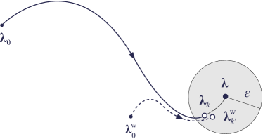
Figure 1: Illustration of improved convergence by warm starting.

2 PGS for nonsmooth discrete element simulation

The mixed complementarity problem (MCP) for computing the update of the velocity from ${\textbf{v}}_{\text{old}}\equiv\bm{v}(t-\Delta t)$ to $\textbf{v}\equiv\bm{v}(t)$ and the Lagrange multiplier $\bm{\lambda}$ of the contact constraints and take the form

$$\left[\begin{array}[c]{cc}\textbf{M}&-\textbf{G}^{\text{T}}\\ \textbf{G}&\bm{\Sigma}\end{array}\right]\left[\begin{array}[c]{c}\textbf{v}\\ \bm{\lambda}\end{array}\right]=\left[\begin{array}[c]{c}\textbf{p}\\ \textbf{q}\end{array}\right]$$ (1)

$$\bm{\lambda}^{(\alpha)}\in\mathcal{C}_{\mu}({\lambda}_{\text{n}}^{(\alpha)})\ \ ,\ \alpha=1,2,\ldots,{N}_{\text{c}}$$ (2)

where $\bm{M}$ is the mass matrix and $\bm{G}$ the Jacobian of contact constraints. The contact force, $\bm{G}^{T}\bm{\lambda}$, is restricted by a friction cone condition that we represent $\bm{\lambda}^{(\alpha)}\in\mathcal{C}_{\mu}({\lambda}_{\text{n}}^{(\alpha)})$, where $\alpha$ indexes the contacts. The diagonal perturbation $\bm{\Sigma}$ regularize the problem and allow modeling of contact elasticity. The vectors $\bm{p}$ and $\bm{q}$ on the right hand side depend on particle inertia, external force and constraint violations on position and velocity level. As friction cone condition we use the Signorini-Coulomb law including $0\leq{\lambda}_{\text{n}}^{(\alpha)}$ and $|\bm{\lambda}_{\text{t}}^{(\alpha)}|\leq{\mu}_{\text{s}}|\textbf{G}_{\text{n}}^{(\alpha){\text{T}}}\lambda_{\text{n}}^{(\alpha)}|$ with the friction coefficient ${\mu}_{\text{s}}$ for each contact $\alpha$ divided in one normal (n) and two tangential (t) components. The constraint forces act to prevent contact overlap, $\bm{g}\leq 0$, and contact sliding, ${\bm{G}}_{\text{t}}\bm{v}=0$. Similarly, rolling resistance (r) is imposed by a constraint ${\bm{G}}_{\text{r}}\bm{v}=0$ with a Coulomb like law: $|\bm{\lambda}_{\text{r}}^{(\alpha)}|\leq{\mu}_{\text{r}}r^{*}|\textbf{G}_{\text{n}}^{(\alpha){\text{T}}}\lambda_{\text{n}}^{(\alpha)}|$, where $r^{*}$ is the effective radius. See Appendix A for further details. For a system with ${N}_{\text{p}}$ particles represented as rigid bodies and ${N}_{\text{c}}$ contacts with normal and tangential force and rolling and twisting resistance the vectors and matrices in Eq. (1) have the following dimensions $\dim(\bm{M})=6{N}_{\text{p}}\times 6{N}_{\text{p}}$, $\dim(\bm{G})=6{N}_{\text{c}}\times{N}_{\text{p}}$, $\dim(\bm{}v)=\dim(\bm{p})=6{N}_{\text{p}}$ $\dim(\bm{\lambda})=\dim(\bm{q})=6{N}_{\text{c}}$. The matrices are however very sparse. $\bm{M}$ and $\bm{\Sigma}$ are block diagonal and $\bm{G}$ is block sparse. The blocks have dimension $6\times 6$. The main steps of the PGS iteration are

$$\bm{\lambda}^{(\alpha)}_{k+1} = \bm{\lambda}^{(\alpha)}_{k}+D^{-1}_{(\alpha\alpha)}\textbf{r}^{(\alpha)}_{k}$$ (3)

$$\bm{\lambda}^{(\alpha)}_{k+1} \leftarrow \text{proj}_{\mathcal{C}_{\mu}}(\bm{\lambda}^{(\alpha)}_{k+1})$$ (4)

$$\textbf{v}_{k+1} = \textbf{v}_{k}+\textbf{M}^{-1}\textbf{G}_{(\alpha)}^{\text{T}}\Delta\bm{\lambda}_{k+1}^{(\alpha)}$$ (5)

with iteration index $k=0,1,2,\ldots,{N}_{\text{it}}-1$, change in multiplier $\Delta\bm{\lambda}_{k+1}^{(\alpha)}=\bm{\lambda}_{k+1}^{(\alpha)}-\bm{\lambda}_{k}^{(\alpha)}$ and residual

$$\textbf{r}^{(\alpha)}_{k}=\textbf{S}_{(\alpha\alpha)}\bm{\lambda}^{(\alpha)}_{k}+\textbf{G}_{(\alpha)}\textbf{M}^{-1}\textbf{p}_{(\alpha)}-\textbf{q}_{(\alpha)}=\textbf{G}_{(\alpha)}\textbf{v}_{k}-\textbf{q}_{(\alpha)}$$ (6)

where $\textbf{v}_{k}\equiv\textbf{M}^{-1}\textbf{p}+\textbf{M}^{-1}\textbf{G}_{(\alpha)}^{\text{T}}\bm{\lambda}_{k}^{(\alpha)}$ and D is the block diagonal part of the Schur complement matrix $\textbf{S}=\textbf{G}\textbf{M}^{-1}\textbf{G}^{\text{T}}+\bm{\Sigma}$. The details of the vectors p and q depend on the stepping scheme and constraint stabilization method. When integrating with fix timesteps $\Delta t$ using the SPOOK stepper lacoursiere:2007:rvs one has $\textbf{p}=\textbf{M}{\textbf{v}}_{\text{old}}+\Delta t{\textbf{f}}_{\text{ext}}$, with smooth external forces ${\textbf{f}}_{\text{ext}}$, and $\textbf{q}=(\textbf{q}^{T}_{\text{n}},\textbf{q}^{T}_{\text{t}},\textbf{q}^{T}_{\text{r}})^{T}$ with $\textbf{q}_{\text{n}}=-(4/\Delta t)\bm{\Upsilon}\bar{\textbf{g}}+\Upsilon\textbf{G}_{\text{n}}{\textbf{v}}_{\text{old}}$, $\textbf{q}_{\text{t}}=\textbf{0}$ and $\textbf{q}_{\text{r}}=\textbf{0}$. The projection $\bm{\lambda}^{(\alpha)}_{k+1}\leftarrow\text{proj}_{\mathcal{C}_{\mu}}(\bm{\lambda}^{(\alpha)}_{k+1})$ is made by simply clamping $\bm{\lambda}^{(\alpha)}_{k+1}$ to the friction or rolling resistance limit if exceeded. After stepping the velocities and positions an impact stage follows. This include solving a MCP similar to Eq. (1) but with the Newton impact law, ${\textbf{G}}_{\text{n}}^{(\alpha)}\textbf{v}_{+}=-e{\textbf{G}}_{\text{n}}^{(\alpha)}\textbf{v}_{-}$, replacing the normal constraints for the contacts with normal velocity larger than an impact velocity threshold ${v}_{\text{imp}}$. The remaining constraints are maintained by imposing $\textbf{G}\textbf{v}_{+}=0$. An algorithm of NDEM simulation with PGS is given in Appendix A together with details on the Jacobians and relation between the solver parameters and material parameters.

3 PGS warm starting

By default the PGS algorithm is initialized with $\bm{\lambda}^{(\alpha)}_{0}=\textbf{0}$. We refer to this as cold starting. In a stationary state the contact force $\textbf{G}^{T}\bm{\lambda}$ is constant in time. In a nearly stationary state we expect the multipliers to remain almost constant between two timestep. Therefore it is reasonable to use the solution from last timestep as an initial guess, $\bm{\lambda}(t)\approx\bm{\lambda}(t-\Delta t)$. We use a fraction $\beta=0.85$ of the solution from last timestep

$$\bm{\lambda}_{0}(t)=\beta\bm{\lambda}_{{N}_{\text{it}}}(t-\Delta t)$$ (7)

It is important to also apply the corresponding impulse to the particles and update the velocity

$$\textbf{v}_{0}=\textbf{M}^{-1}\textbf{p}+\textbf{M}^{-1}\textbf{G}^{\text{T}}\bm{\lambda}_{0}$$ (8)

such it become consistent with the initial guess for the multiplier. We refer to warm starting based on the last solution as history based warm starting. For any new contact we set $\bm{\lambda}^{(\alpha)}_{0}=\textbf{0}$. Warm starting is not applied at the impact stage and we assume that the contact network is not fundamentally rearranged by the impacts and use the solution from last timestep despite the occurrence of impacts.

An alternative method for warm starting a nearly stationary state is to estimate each local contact force and assign this to the contact multipliers. When using regularized NDEM the local contact force can be estimated from the overlaps and relative contact velocities much as in conventional smooth DEM. We refer to this approach as model based warm starting. For normal forces we use the Hertz contact law ${f}_{\text{n}}={k}_{\text{n}}g^{3/2}_{\text{n}}$, with overlap function $g_{\text{n}}$ and based on ${\textbf{f}}_{\text{n}}\approx{\textbf{G}}_{\text{n}}^{T}{\bm{\lambda}}_{\text{n}}/\Delta t$ we estimate

$$\lambda_{\text{n},0}^{(\alpha)}\approx\tfrac{5}{4}\Delta t{k}_{\text{n}}g^{5/4}_{\text{n}(\alpha)}$$ (9)

Similarly the regularized tangent friction force and rolling resistance force can be estimated via the Rayleigh dissipation functions to

$$\bm{\lambda}_{\text{t},0} \approx {\gamma}_{\text{t}}^{-1}\Delta t({\textbf{G}}_{\text{t}}\textbf{v})^{\text{T}}{\textbf{G}}_{\text{t}}$$ (10)

$$\bm{\lambda}_{\text{r},0} \approx {\gamma}_{\text{r}}^{-1}\Delta t({\textbf{G}}_{\text{r}}\textbf{v})^{\text{T}}{\textbf{G}}_{\text{r}}$$ (11)

Note that the friction and rolling resistance should, if large, be clamped to obey the conditions $|\bm{\lambda}_{\text{t}}^{(\alpha)}|\leq{\mu}_{\text{s}}|\textbf{G}_{\text{n}}^{(\alpha){\text{T}}}\lambda_{\text{n}}^{(\alpha)}|$ and $|\bm{\lambda}_{\text{r}}^{(\alpha)}|\leq{\mu}_{\text{r}}r^{*}|\textbf{G}_{\text{n}}^{(\alpha){\text{T}}}\lambda_{\text{n}}^{(\alpha)}|$.

4 Numerical experiments

Numerical simulation of different systems were performed to analyse the effect of warm starting on the convergence of NDEM simulations. The following systems were studied: a 1D column, formation of a pile, dense flow in a rotating drum and a triaxial shear cell. The main material and simulation parameters are listed in Table 1. The method was implemented in the software AgX Dynamics agx in the module for NDEM simulation with optimized data structures and support for collision detection and PGS using parallel computing on multicore processors. The simulations were run on a desktop computer with Intel(R) Core(TM) i7 CPU, 2.8 GHz, 8 GB RAM on a Windows 64 bit system. Videos from simulations are found at http://umit.cs.umu.se/granular/warmstarting/.

Table 1: Main material and simulation parameters

Notation	Value	Comment
$[d,d_{2}]$	$[13,10]$ m	bi-disperse particle diameter
$\rho$	$3700$ kg/m3	particle mass density
$E$	$6$ MPa	Young’s modulus
$e$	$0.18$	restitution coefficient
${\mu}_{\text{s}}$	$0.91$	surface friction coefficient
${\mu}_{\text{r}}$	$0.32$	rolling resistance coefficient
$\Delta t$	$5$ ms	timestep
${v}_{\text{imp}}$	$0.05$ m/s	impact threshold

4.1 Column

Particles of diameter $d=13$ mm are initiated on top of another with zero overlap. The system compress slightly under its weight. The simulation is run until the 1D column have come to rest. Sample images from simulation with and without warm starting and for different number of iterations are shown in Fig. 2. Warm starting clearly improve the convergence.

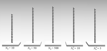
Figure 2: Samples of five columns simulated, from left to right, with cold starting ${N}_{\text{it}}=10,50$ and $500$, and history based warm starting $N^{\text{w}}_{\text{it}}=10$ and $5$.

To make a quantitative convergence analysis we study the deviation of the simulated column height, $l_{{N}_{\text{it}}}$, from the theoretical height, $l$, computed using the Hertz contact law

$${\varepsilon}_{\text{l}}=\frac{l-l_{{N}_{\text{it}}}}{l}$$ (12)

A series of simulations are run with number of particles, ${N}_{\text{P}}$, ranging from $5$ and $100$, number of iterations, ${N}_{\text{it}}$, ranging from $10$ to $500$. The required number of iterations, ${N}_{\text{it}}^{\varepsilon}$, to reach a solution with error tolerance ${\varepsilon}_{\text{l}}=0.1\%,1\%$ and $5\%$ are presented in Fig. 3. It scales almost linearly with the number of particles and increase with decreasing error tolerance ${\varepsilon}_{\text{l}}$. History based warm starting is on average three times as efficient as cold starting. Also model based warm starting improve the convergence at low error tolerance. The performance gain from model based warm starting decrease with increasing error tolerance and for ${\varepsilon}_{\text{l}}=5\%$ model based warm starting require twice as many iterations as cold starting.

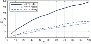
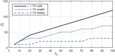
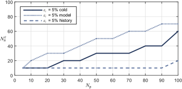
Figure 3: The required number of iterations for a 1D column simulation for error tolerance ${\varepsilon}_{\text{1D}}=0.1\%$ (top), $1\%$ (middle) and $5\%$ (bottom) depending on the number of particles and warm starting method.

Figure 4 show the evolution of the mean residual, see Eq. (6), for the normal force constraint during a PGS solve for a column with ${N}_{\text{p}}=25$. The convergence rates are similar but warm starting clearly has the advantage of starting closer to the solution.

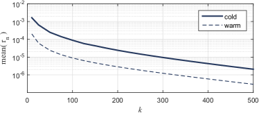
Figure 4: The evolution of the mean normal force residual during a PGS solve for a ${N}_{\text{p}}=25$ column using cold starting and history based warm starting.

4.2 Pile formation

A pile is formed by continuously emitting particles of diameter $d=13$ mm from a $3d$ wide source placed $20d$ above a ground plane. The number of particles in the pile is ${N}_{\text{p}}=3363$. Again we use the relative height, ${\varepsilon}_{\text{l}}$ in Eq. (12), as error measurement. The reference height about $15d$ is measured from a pile constructed using small time-step $\Delta t=0.2$ ms and ${N}_{\text{it}}=500$. Pile formation is then simulated using time-step $\Delta t=5$ ms for different number of iterations and warm starting methods. Sample images from simulations are shown in Fig. 5.

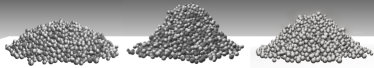
Figure 5: Samples from simulations of pile formation. From left to right is the cold started pile ($\Delta t=5$ ms, ${N}_{\text{it}}=50$), a reference pile ($\Delta t=0.2$ ms, ${N}_{\text{it}}=500$) and a warm started pile ($\Delta t=5$ ms, ${N}_{\text{it}}=50$)

The angle of repose is an alternative measure but was found to give less precise result. The pile height is measured $10$ s after the last emitted particle has come to approximate rest. Simulations are run with warm starting applied both to normal forces, friction and rolling resistance and to normal forces only. The historical warm starting is tested with and without the velocity update associated with the warm start in Eq. (7). The required number of iterations for a given error threshold are given in Fig. 6. With few iterations the piles experience artificial compression and contact sliding such that the pile gradually melt down to a singe particle layer. The pile stability increase with the number of iterations. History based warm starting, applied to both normals, friction and rolling resistance, give the best result and require roughly half the number of iterations of cold starting. If the warm start velocity is not applied the result is worse than cold starting. Model based warm starting is only marginally better than cold starting and is from further experiments here on excluded. Applying warm starting to the normal constraints only does not improve the convergence significantly.

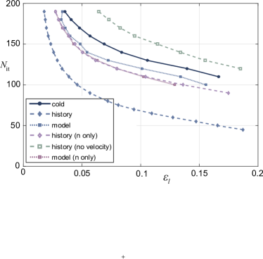
Figure 6: The required number of iterations versus pile height error for different warm starting methods.

The convergence is also analysed by studying the evolution of the Lagrange multiplier and the residual. The relative error of the normal force multiplier is computed as

$$\varepsilon_{\lambda_{k}}=\left\langle\frac{|\bm{\lambda}^{\text{n}(\alpha)}_{500}-\bm{\lambda}^{\text{n}(\alpha)}_{k}|}{|\bm{\lambda}^{\text{n}(\alpha)}_{500}|}\right\rangle$$ (13)

The evolution of $\varepsilon_{\lambda_{k}}$ during a solve of a stationary pile is shown in Fig. 7. The multiplier error for history based warm starting is roughly five times smaller than for cold starting and remain more accurate indefinitely.

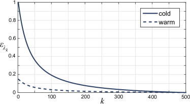
Figure 7: The evolution of the relative multiplier during a PGS solve for a resting pile using cold starting and history based warm starting.

A more careful analysis can be made by studying the evolution of the residual, defined in Eq. (6), and how it is distributed over the constraints. To get comparable states a stationary pile is prepared by using 500 iterations from which the cold and warm started simulations are started and run for $1$ s before the measurement. The evolution of the mean residual during a PGS solve is shown in Fig. 8. The convergence rates are similar but the initial lead of history based warm starting over cold starting by roughly a factor $5$ remains throughout the 500 PGS iterations. Comparing the residual histograms from using cold and warm starting in Fig. 9 it is clear that the solutions differs primarily in the errors for the rolling resistance and friction constraints and less so for normal force constraints. This is consistent with the faster melting of the piles simulated with cold starting.

Figure 8: The mean residual dependency on the number of iterations when simulating a resting pile for $1$ s using cold starting and history based warm starting.

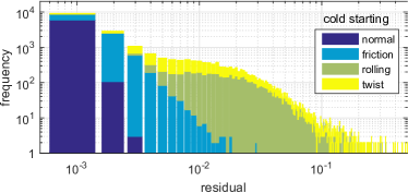
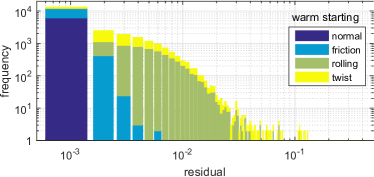
Figure 9: The residual distribution for a resting pile after $1$ s using ${N}_{\text{it}}=100$ iterations, cold starting (top) and history based warm starting (bottom).

4.3 Rotating drum

A cylindrical drum with diameter $D=40d$ and width $w=7d$ is rotated with angular velocity $\Omega=0.25$ rad/s. This corresponds to the Froude number $\text{Fr}\equiv D\Omega^{2}/2g\sim 10^{-3}$ which corresponds to the dense rolling flow regime. A nearly stationary flow of ${N}_{\text{p}}=4864$ particles with bi-disperse size distribution $d$ and $d_{2}$. At this low Froude number a large plug-zone is developed where particles co-rotate rigidly with the drum. A convergence analysis is made of the plug-zone number fraction, ${N}_{\text{plug}}/{N}_{\text{p}}$, and the dynamic angle of repose, $\theta^{\prime}$. These are measured for different number of iterations on a flow averaged over $2$ s for cold starting and historical warm starting. The sample trajectories in Fig. 10 illustrate the general trend that the dynamic angle of repose and the size of the plug zone decrease with decreasing number of iterations but less so using warm starting.

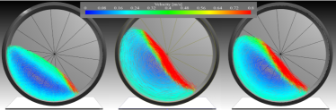
Figure 10: A sample of particle trajectories from simulation of a rotating drum with $\Omega=0.25$ rad/s, $\Delta t=5$ ms and ${N}_{\text{it}}=10$ (left), ${N}_{\text{it}}=500$ (middle) and warm starting ${N}_{\text{it}}=10$ (right).

The normalized particle flow velocity relative the plug flow is computed ${v}_{\text{r}}^{i}\equiv|\textbf{v}^{i}-\textbf{r}^{i}\times\bm{\Omega}|/R\Omega$ and sample plots are shown in Fig. 11. As threshold for the plug zone flow we set ${v}_{\text{r}}\leq 0.15$, which is fulfilled by ${N}_{\text{plug}}^{500}/{N}_{\text{p}}=58\%\pm 5\%$ particles where the variations reflect the slightly pulsating nature of the flow, due to sequential onset of avalanches. The plug zone fraction number error is defined

$${\varepsilon}_{\text{plug}}=\frac{{N}_{\text{plug}}^{500}-N_{\text{plug}}^{{N}_{\text{it}}}}{{N}_{\text{p}}}$$ (14)

and the relation to the required number of iterations is found in Fig. 12. The warm starting solution approach the solution faster but seems to have larger variations at high iteration numbers.

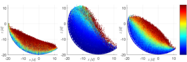
Figure 11: A sample of cross-section flow from a simulation of a rotating drum with $\Omega=0.25$ rad/s, $\Delta t=5$ ms and ${N}_{\text{it}}=10$ (left), ${N}_{\text{it}}=500$ (middle) and warm starting ${N}_{\text{it}}=10$ (right). The colour coding show the particle velocities relative to rigid co-motion with the drum.

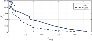
Figure 12: The convergence of the plug zone fraction number for cold starting and history based warm starting.

The convergence analysis of the dynamic angle of repose also show that warm starting converges faster although to a slightly higher angle ${\theta}_{\text{w,plug}}^{500}=50^{\circ}$ compared to ${\theta}_{\text{plug}}^{500}=48^{\circ}$, see Fig. 13. The dynamic angle of repose is measured as the displacement of the material centre of mass from the $z$-axis which is more robust than tracking the surface.

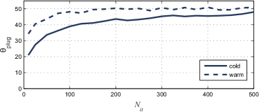
Figure 13: The dynamic angle of repose as function of number of iterations for cold starting and history based warm starting.

4.4 Triaxial shear

The triaxial shear test is constructed by six dynamic rigid walls of mass $100$ kg each that are driven with prismatic motors to apply a specific stress $\sigma_{i}=f_{i}/A_{i}$, where $A_{i}$ is the cross-section area and $f_{i}$ the applied motor force in the coordinate direction $i=x,y,z$, see Fig. 14

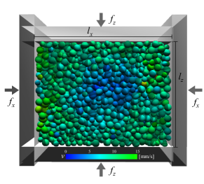
Figure 14: Sample image from the triaxial test.

First, a hydrostatic pressure of ${\sigma}^{\text{h}}=100$ Pa is applied on all sides. Then the top and bottom walls are driven inwards at $0.01$ m/s by regulating $\sigma_{z}$ and maintaining a constant side wall pressure at $\sigma_{x}=\sigma_{y}={\sigma}^{\text{h}}$. At some critical deviator stress ${\sigma}^{\text{c}}_{z}-{\sigma}^{\text{h}}$ the material fail to sustain further increase in stress and starts to shear indefinitely. The transition is more or less sharp depending on the initial packing ratio, hydrostatic pressure and applied shear rate. In this test the Young’s modulus is set to the stiffer value of $E=60$ MPa to get a sharper transition between compression and shear. The critical axial stress ${\sigma}^{\text{c}}_{z}$ is computed as the averaged $\sigma_{z}$ in the shear phase between lateral strain $\varepsilon=10\%$ to $\varepsilon=25\%$. The critical stress deviator depending on the number of iterations for cold starting and history based warm starting is shown in Fig. 15. Both curves converge to about $1\pm 0.2$ kPa. With warm starting the stress levels out at ${N}_{\text{it}}\gtrsim 200$ while cold starting require ${N}_{\text{it}}=1000$.

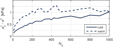
Figure 15: Critical yield stress as function of number of iterations for cold starting and history based warm starting.

Sample curves of the stress deviator as function of lateral strain are shown in Fig. 16. These confirm the faster convergence when warm starting but also show higher stress fluctuations in the shear phase. Whether this is an artefact of the warm starting or an actual feature of the triaxial test has not been pursued.

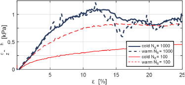
Figure 16: Sample stress curves in triaxial test for 100 and 1000 iterations.

5 Application example

The effect of using warm starting in practical simulation applications is illustrated with two examples. The first example is part of a balling drum circuit used in ore pelletizing systems wang:2015:pvn , see Fig. 17. Simulations are used for the purpose of process control and for finding a design of the drum outlet that maximizes an evenly distributed throughput on a roller sieve where material is size distributed. Three distinctive subsystems with different dynamics can be identified. Firstly, there is the drum with an almost stationary flow. Secondly, material is distributed onto quasistationary piles on a wide-belt conveyor. Thirdly, the particles disperse over a roller sieve with increasing gap size downwards to achieve a size separation. The design problem is fore mostly a geometric flow problem and the material distribution need to be computed with sufficient accuracy. We assume $5$ % is a required accuracy for dynamic and static angle of repose. From Fig. 13 we estimate that warm starting is roughly three times more computationally efficient in computing the drum flow and, according to Fig. 6, twice as efficient for pile formation on the conveyor. The flow on the roller sieve is more disperse and collision dominated requiring only few iterations (${N}_{\text{p}}<25$) and it can be expected that warm and cold starting are equally efficient. The overall computational speed-up by applying warm starting is thus estimated to a factor no larger than 2.

The second example is an excavator. A rectangular trench is filled with roughly $10^{5}$ spherical particles of uniform size distribution between $25$ and $100$ mm and particle mass density of $2500$ kg/m³. The excavator is modeled as a rigid multibody system of total mass $50$ ton divided in 10 bodies, 8 joints and 3 linear actuators (hydraulic cylinders) and one rotational motor. The full system of granulars and vehicle take the mathematical form of Eq. (1) and is solved using a split solver where the vehicle part is solved using a direct block-sparse pivoting method agx and the granular material with a PGS solver as described in this paper. Simulations were run with time-step $h=2.5$ ms, which allow for a low number of iterations. The machine perform an excavation cycle by a pre-programmed control signal to the actuators. The resulting actuator forces are measured and these include the back reaction from the resistance and inertia of the granular material. Two simulations, with and without warm starting, are run with ${N}_{\text{it}}=25$. Sample images from the simulations are shown in Fig. 18. Observe the difference in height surface of the granular material due to artificial compression and frictional slippage due to numerical errors in the PGS solve. The undisturbed height in the two simulations differ by $10$ % and volume of displaced material differ by at least $30$ %. The difference in granular dynamics also affect the measured force response. The force trajectory of the middle actuator is provided in Fig. 19. In the phase between $8\--10$ s, when the bucket is dragged through the material the force when using warm starting is almost $50\%$ larger because more material is set in motion and stronger resistance to shear motion. Whether $h=2.5$ ms, ${N}_{\text{it}}=25$ and the improvement by using warm starting give sufficiently accurate force response depend on the intended use of the data and require further convergence analysis. On a desktop computer with the given NDEM settings the computational time is roughly $100$ s per realtime second.

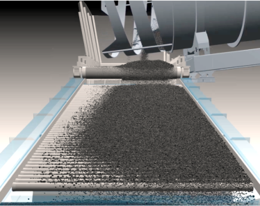
Figure 17: A balling drum circuit with granular material in different states.

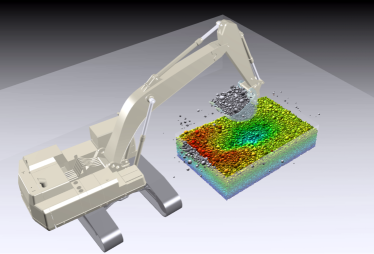
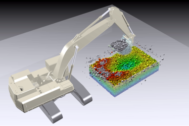
Figure 18: An excavator digging in trench with $~{}10^{5}$ particles, $h=2.5ms$, ${N}_{\text{it}}=25$ and using cold starting (top) and warm starting (bottom). The colour codes the particle height with red to blue ranging from $0$ m to $-2$ m. Gray particles are above $0$ m.

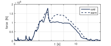
Figure 19: The force trajectory of the middle link pistons of the excavator while digging with ${N}_{\text{it}}=25$ using cold starting and warm starting.

6 Conclusions

The convergence of the projected Gauss-Seidel algorithm for NDEM simulation is increased by warm starting with the solution from previous time-step. The computational speed-up by warm starting is demonstrated to be about $2\--5$ for a wide range of systems including pile formation, granular drum flow and triaxial shear. An examination of the residual distribution show that convergence improvement primarily improve on the velocity constraints - friction and rolling resistance - and less so on the normal force constraints. Warm starting the Lagrange multiplier based on $85$ % of the value from last time-step was found to give best results. Warm starting based on an explicit contact force model give only marginal speed-up, for example $20$ % for a pile formation. This is not surprising since the damping coefficients in the dissipation models for sliding and rolling are not physics based and can only predict the value of contact forces in slide mode but not of stick mode inside the friction and rolling resistance limits. For materials shearing under high stress, compared to the stress produced by the materials own weight, warm starting show larger stress fluctuations than without warm starting. Whether this is an artefact or correct behaviour emerging after further iterations has not been established. A more in depth analysis of systems under large stress should be made considering also alternative size of time step, shear rate, hydrostatic load stress and particle stiffness.

Appendix

A. Simulation algorithm

The algorithm for simulating a system of granular material using NDEM with PGS solver with warm starting is given in Algorithm 1.

Algorithm 1 NDEM simulation with warm started PGS solver

1:set constants and parameters

2:initial state: $(\textbf{x}_{0},\textbf{v}_{0})$

3:for $i=0,1,2,\ldots,t/\Delta t$ do $\triangleright$ Time stepping

4:     contact detection

5:     compute $\textbf{g},\textbf{G},\bm{\Sigma},\textbf{D}$

6:     impact stage PGS solve $\textbf{v}_{i}\to(\textbf{v}^{+}_{i},\bm{\lambda}^{+}_{i})$ $\triangleright$ impacts

7:     compute ${\textbf{q}}_{\text{n}}=-(4/\Delta t){\bm{\Upsilon}}_{\text{n}}{\textbf{g}}_{\text{n}}+{\bm{\Upsilon}}_{\text{n}}{\textbf{G}}_{\text{n}}\textbf{v}^{+}_{i}$

8:     pre-step $\textbf{v}=\textbf{v}^{+}_{i}+\Delta t\textbf{M}^{-1}{\textbf{f}}_{\text{ext}}$

9:     $\bm{\lambda}_{k_{0}}=\textbf{0}$ or warm start $\bm{\lambda}_{k_{0}}$

10:     warm-step $\textbf{v}=\textbf{v}+\textbf{M}^{-1}\textbf{G}^{\text{T}}\bm{\lambda}_{k_{0}}$

11:     $---$ $\triangleright$ PGS solve for continuous contacts$----$

12:     for $k=1,\ldots,{N}_{\text{it}}$ and while criteria$(\textbf{r})$ do

13:         for each contact $\alpha=0,1,\ldots,{N}_{\text{c}}-1$ do

14:              for each constraint $n$ of contact $\alpha$ do

15:                  $\textbf{r}^{(\alpha)}_{n,k}=-\textbf{q}^{(\alpha)}_{n,k}+\textbf{G}^{(\alpha)}_{n}\textbf{v}$ $\triangleright$ residual

16:                  $\bm{\lambda}^{(\alpha)}_{n,k}=\bm{\lambda}^{(\alpha)}_{n,k-1}+\textbf{D}^{-1}_{n,(\alpha)}\textbf{r}^{(\alpha)}_{n,k}$ $\triangleright$ multiplier

17:                  $\bm{\lambda}^{(\alpha)}_{n,k}\leftarrow\text{proj}_{\mathcal{C}_{\mu}}(\bm{\lambda}^{(\alpha)}_{k})$ $\triangleright$ project

18:                  $\Delta\bm{\lambda}^{(\alpha)}_{n,k}=\bm{\lambda}^{(\alpha)}_{n,k}-\bm{\lambda}^{(\alpha)}_{n,k-1}$

19:                  $\textbf{v}=\textbf{v}+\textbf{M}^{-1}\textbf{G}^{T}_{n,(\alpha)}\Delta\bm{\lambda}^{(\alpha)}_{n,k}$

20:              end for

21:         end for

22:     end for

23:     $\textbf{v}_{i+1}=\textbf{v}$ $\triangleright$ velocity update

24:     $\textbf{x}_{i+1}=\textbf{x}_{i}+\Delta t\textbf{v}_{i+1}$ $\triangleright$ position update

25:end for

Based on the Hertz contact law, each contact $\alpha$ between body $a$ and $b$ add contributions to the constraint vector and normal and friction Jacobians according to

$$\delta_{(\alpha)} = \mathbf{n}_{(\alpha)}^{\text{T}}(\mathbf{x}_{a}+\mathbf{d}^{(\alpha)}_{a}-\mathbf{x}_{b}-\mathbf{d}^{(\alpha)}_{b})$$

$$g_{(\alpha)} = \delta^{{e}_{\text{H}}}_{(\alpha)}\quad,\ {e}_{\text{H}}=5/4$$

$$\textbf{G}_{\text{n}a}^{(\alpha)} = {e}_{\text{H}}g^{{e}_{\text{H}}-1}_{(\alpha)}\left[\begin{array}[c]{cc}-\mathbf{n}_{(\alpha)}^{{\text{T}}}&\ \ -(\mathbf{d}^{(\alpha)}_{a}\times\mathbf{n}_{(\alpha)})^{\text{T}}\end{array}\right]$$ (16)

$$\textbf{G}_{\text{n}b}^{(\alpha)} = {e}_{\text{H}}g^{{e}_{\text{H}}-1}_{(\alpha)}\left[\begin{array}[c]{cc}\mathbf{n}_{(\alpha)}^{{\text{T}}}&\ \ (\mathbf{d}^{(\alpha)}_{b}\times\mathbf{n}_{(\alpha)})^{\text{T}}\end{array}\right]$$ (18)

$$\textbf{G}_{\text{t}a}^{(\alpha)} = \left[\begin{array}[c]{cc}-\mathbf{t}^{(\alpha){\text{T}}}_{1}&\ \ -(\mathbf{d}^{(\alpha)}_{a}\times\mathbf{t}^{(\alpha)}_{1})^{\text{T}}\\ -\mathbf{t}^{(\alpha){\text{T}}}_{2}&\ \ -(\mathbf{d}^{(\alpha)}_{a}\times\mathbf{t}^{(\alpha)}_{2})^{\text{T}}\end{array}\right]$$ (21)

$$\textbf{G}_{\text{t}b}^{(\alpha)} = \left[\begin{array}[c]{cc}\mathbf{t}^{(\alpha){\text{T}}}_{1}&\ \ (\mathbf{d}^{(\alpha)}_{b}\times\mathbf{t}^{(\alpha)}_{1})^{\text{T}}\\ \mathbf{t}^{(\alpha){\text{T}}}_{2}&\ \ (\mathbf{d}^{(\alpha)}_{b}\times\mathbf{t}^{(\alpha)}_{2})^{\text{T}}\end{array}\right]$$ (24)

$$\textbf{G}_{\text{r}a}^{(\alpha)} = \left[\begin{array}[c]{cccc}\mathbf{0}_{1\times 3}&\ \ \mathbf{t}^{(\alpha){\text{T}}}_{1}&\ \ \mathbf{0}_{1\times 3}&-\mathbf{t}^{(\alpha){\text{T}}}_{1}\\ \mathbf{0}_{1\times 3}&\ \ \mathbf{t}^{(\alpha){\text{T}}}_{2}&\ \ \mathbf{0}_{1\times 3}&-\mathbf{t}^{(\alpha){\text{T}}}_{2}\\ \mathbf{0}_{1\times 3}&\ \ \mathbf{n}^{(\alpha){\text{T}}}&\ \ \mathbf{0}_{1\times 3}&-\mathbf{n}^{(\alpha){\text{T}}}\\ \end{array}\right]$$ (28)

$$\textbf{G}_{\text{r}b}^{(\alpha)} = \left[\begin{array}[c]{cccc}\mathbf{0}_{1\times 3}&\ \ -\mathbf{t}^{(\alpha){\text{T}}}_{1}&\ \ \mathbf{0}_{1\times 3}&\mathbf{t}^{(\alpha){\text{T}}}_{1}\\ \mathbf{0}_{1\times 3}&\ \ -\mathbf{t}^{(\alpha){\text{T}}}_{2}&\ \ \mathbf{0}_{1\times 3}&\mathbf{t}^{(\alpha){\text{T}}}_{2}\\ \mathbf{0}_{1\times 3}&\ \ -\mathbf{n}^{(\alpha){\text{T}}}&\ \ \mathbf{0}_{1\times 3}&\mathbf{n}^{(\alpha){\text{T}}}\\ \end{array}\right]$$ (32)

where $\textbf{d}^{(\alpha)}_{a}$ and $\textbf{d}^{(\alpha)}_{b}$ are the positions of the contact point $\alpha$ relative to the particle positions $\textbf{x}_{a}$ and $\textbf{x}_{b}$. The orthonormal contact normal and tangent vectors are $\mathbf{n}^{(\alpha)}$, $\mathbf{t}^{(\alpha)_{1}}$ and $\mathbf{t}^{(\alpha)_{2}}$.

The diagonal matrices and Schur complement matrix D are

$${\bm{\Sigma}}_{\text{n}} = \frac{4}{\Delta t^{2}}\frac{{\varepsilon}_{\text{n}}}{1+4\tfrac{{\tau}_{\text{n}}}{\Delta t}}\bm{1}_{N_{c}\times N_{c}}$$

$${\bm{\Sigma}}_{\text{t}} = \frac{{\gamma}_{\text{t}}}{\Delta t}\bm{1}_{2N_{c}\times 2N_{c}}$$

$${\bm{\Sigma}}_{\text{r}} = \frac{{\gamma}_{\text{r}}}{\Delta t}\bm{1}_{3N_{c}\times 3N_{c}}$$ (33)

$${\bm{\Upsilon}}_{\text{n}} = \frac{1}{1+4\tfrac{{\tau}_{\text{n}}}{\Delta t}}\bm{1}_{N_{c}\times N_{c}}$$

D $$= \textbf{G}\textbf{M}^{-1}\textbf{G}^{T}+\bm{\Sigma}$$

The mapping between MCP parameters and material parameters are

$${\varepsilon}_{\text{n}} = {e}_{\text{\tiny H}}/{k}_{\text{n}}=3{e}_{\text{\tiny H}}(1-\nu^{2})/E\sqrt{r^{*}}$$

$${\tau}_{\text{n}} = \max({n}_{\text{s}}\Delta t,{\varepsilon}_{\text{n}}/{\gamma}_{\text{n}})$$ (34)

$${\gamma}_{\text{n}}^{-1} = {k}_{\text{n}}c/e^{2}_{\text{\tiny H}}$$

where $r^{*}=(r_{a}+r_{b})/r_{a}r_{b}$ is the effective radius and we use ${\gamma}_{\text{t}}={\gamma}_{\text{r}}=10^{-6}$, ${n}_{\text{s}}=2$.

References

- (1) J. J. Moreau. Numerical aspects of the sweeping process. Computer Methods in Applied Mechanics and Engineering, 177:329–349, July 1999.
- (2) M. Jean. The non-smooth contact dynamics method. Computer Methods in Applied Mechanics and Engineering, 177:235–257, July 1999.
- (3) Farhang Radjai and Vincent Richefeu. Contact dynamics as a nonsmooth discrete element method. Mechanics of Materials, 41(6):715–728, June 2009.
- (4) B Brogliato, Aa Ten Dam, L Paoli, F Génot, and M Abadie. Numerical simulation of finite dimensional multibody nonsmooth mechanical systems. Applied Mechanics Reviews, 55(2):107–150, 2002.
- (5) T. Unger, L. Brendel, D. Wolf, and J. Kertï¿œsz. Elastic behavior in contact dynamics of rigid particles. Physical Review E, 65(6):7, 2002.
- (6) T. Precklik, U. Rude Ultrascale simulations of non-smooth granular dynamics, Comp. Part. Mech., DOI 10.1007/s40571-015-0047-6, 2015.
- (7) V. Visseq, P. Alart, D. Dureisseix, High performance computing of discrete nonsmooth contact dynamics with domain decomposition. Int J Numer Methods Eng, 96(9):584–598, 2013.
- (8) D. Kaufman, S. Sueda, D. James, D. Pai, Staggered Projections for Frictional Contact in Multibody Systems, ACM Transactions on Graphics 27 (5) (2008) 164:1–164:11.
- (9) D. Kaufman, Coupled Principles for Computational Frictional Contact Mechanics, Dissertation (2009).
- (10) K. Erleben, Numerical Methods for Linear Complementarity Problems in Physics-based Animation, ACM SIGGRAPH 2013 Courses, 8:1–8:42 (2013).
- (11) A. Moravánszky, P. Terdiman, Fast Contact Reduction for Dynamics Simulation, in Game Programming Gems 4 ed. A. Kirmse, Charles River Media (2004) 253–263.
- (12) E. Todorov, Implicit nonlinear complementarity: A new approach to contact dynamics, 2010 IEEE International Conference on Robotics and Automation (ICRA) (2010) 2322–2329.
- (13) C. Lacoursière, Regularized, stabilized, variational methods for multibodies, in: D. F. Peter Bunus, C. Führer (Eds.), The 48th Scandinavian Conference on Simulation and Modeling (SIMS 2007), Linköping University Electronic Press, 2007, pp. 40–48.
- (14) M. Servin, D. Wang, C. Lacoursière, K. Bodin, Examining the smooth and nonsmooth discrete element approach to granular matter, Int. J. Numer. Meth. Engng. 97 (2014) 878–902.
- (15) Algoryx Simulations. AGX Dynamics, December 2014.
- (16) D. Wang, M. Servin, T. Berglund, K-O. Mickelsson, S. Rönnbäck, Parametrization and validation of a nonsmooth discrete element method for simulating flows of iron ore green pellets, Powder Technology, 283 (2015) 475–487.