Measuring Partial Balance in Signed Networks

Abstract

Is the enemy of an enemy necessarily a friend? If not, to what extent does this tend to hold? Such questions were formulated in terms of signed (social) networks and necessary and sufficient conditions for a network to be “balanced” were obtained around 1960. Since then the idea that signed networks tend over time to become more balanced has been widely used in several application areas. However, investigation of this hypothesis has been complicated by the lack of a standard measure of partial balance, since complete balance is almost never achieved in practice. We formalize the concept of a measure of partial balance, discuss various measures, compare the measures on synthetic datasets, and investigate their axiomatic properties. The synthetic data involves Erdős-Rényi and specially structured random graphs. We show that some measures behave better than others in terms of axioms and ability to differentiate between graphs. We also use well-known datasets from the sociology and biology literature, such as Read’s New Guinean tribes, gene regulatory networks related to two organisms, and a network involving senate bill co-sponsorship. Our results show that substantially different levels of partial balance is observed under cycle-based, eigenvalue-based, and frustration-based measures. We make some recommendations for measures to be used in future work. structural analysis, signed networks, balance theory, axiom, frustration index, algebraic conflict
2000 Math Subject Classification: 05C22, 05C38, 91D30, 90B10

1 Introduction

Transitivity of relationships has a pivotal role in analyzing social interactions. Is the enemy of an enemy a friend? What about the friend of an enemy or the enemy of a friend? Network science is a key instrument in the quantitative analysis of such questions. Researchers in the field are interested in knowing the extent of transitivity of ties and its impact on the global structure and dynamics in communities with positive and negative relationships. Whether the application involves international relationships among states, friendships and enmities between people, or ties of trust and distrust formed among shareholders, relationship to a third entity tends to be influenced by immediate ties.

There is a growing body of literature that aims to connect theories of social structure with network science tools and techniques to study local behaviors and global structures in signed graphs that come up naturally in many unrelated areas. The building block of structural balance is a work by Heider heider_social_1944 that was expanded into a set of graph-theoretic concepts by Cartwright and Harary cartwright_structural_1956 to handle a social psychology problem a decade later. The relationship under study has an antonym or dual to be expressed by the opposite sign harary_structural_1957 . In a setting where the opposite of a negative relationship is a positive relationship, a tie to a distant neighbor can be expressed by the product of signs reaching him. Cycles containing an odd number of negative edges are considered to be unbalanced, guaranteeing total balance therefore only in networks containing no such cycles. This strict condition makes it quite unlikely for a signed network to be totally balanced. The literature on signed networks suggests many different formulae to measure balance. These measures are useful for detecting total balance and imbalance, but for intermediate cases their performance is not clear and has not been systematically studied.

Our contribution

The main focus of this paper is to provide insight into measuring partial balance, as much uncertainty still exists on this. The dynamics leading to specific global structures in signed networks remain speculative even after studies with fine-grained approaches. The central thesis of this paper is that not all measures are equally useful. We provide a numerical comparison of several measures of partial balance on a variety of undirected signed networks, both randomly generated and inferred from well-known datasets. Using theoretical results for simple classes of graphs, we suggest an axiomatic framework to evaluate these measures and shed light on the methodological details involved in using such measures.

This paper begins by laying out the theoretical dimensions of the research in Section 2 and looks at basic definitions and terminology. In Section 3 different means of checking for total balance are outlined. Section 4 discusses some approaches to measuring partial balance in Eq. (10) – (17), categorized into three families of measures 4.1 – 4.3 and summarized in Table 1. Numerical results on synthetic data are provided in Figures 1 – 2 in Section 5. Section 6 is concerned with analytical results on synthetic data in closed-form formulae in Table 2 and visually represented in Figures 3 – 4. Axioms and desirable properties are suggested in Section 7 to evaluate the measures systematically. Section 8 concerns recommendations for choosing a measure of balance. Numerical results on real signed networks are presented in Section 9. Finally, Section 10 summarizes the study and provides direction for future research.

2 Problem statement and notation

Throughout this paper, the terms signed graph and signed network will be used interchangeably to refer to a graph with positive and negative edges. We use the term cycle only as a shorthand for referring to simple cycles of the graph. While several definitions of the concept of balance have been suggested, this paper will only use the definition for undirected signed graphs unless explicitly stated.

We consider an undirected signed network $G=(V,E,\sigma)$ where $V$ and $E$ are the sets of vertices and edges, and $\sigma$ is the sign function $\sigma:E\rightarrow\{-1,+1\}$. The set of nodes is denoted by $V$, with $|V|=n$. The set of edges is represented by $E$ including $m^{-}$ negative edges and $m^{+}$ positive edges adding up to a total of $m=m^{+}+m^{-}$ edges. The symmetric signed adjacency matrix and the unsigned adjacency matrix are denoted by A and ${|\textbf{A}|}$ respectively. Their entries are defined in (3) and (6).

$$a{{}_{u}}{{}_{v}}=\left\{\begin{array}[]{ll}\sigma_{(u,v)}&\mbox{if }{(u,v)}\in E\\ 0&\mbox{if }{(u,v)}\notin E\end{array}\right.$$ (3)

$$|a{{}_{u}}{{}_{v}}|=\left\{\begin{array}[]{ll}1&\mbox{if }{(u,v)}\in E\\ 0&\mbox{if }{(u,v)}\notin E\end{array}\right.$$ (6)

The positive degree and negative degree of node $i$ are denoted by $d^{+}_{i}$ and $d^{-}_{i}$ representing the number of positive and negative edges incident on node $i$ respectively. They are calculated based on $d^{+}_{i}=(\sum_{j}|a_{ij}|+\sum_{j}a_{ij})/2$ and $d^{-}_{i}=(\sum_{j}|a_{ij}|-\sum_{j}a_{ij})/2$. The degree of node $i$ is represented by $d_{i}$ and equals the number of edges incident on node $i$. It is calculated based on $d_{i}=d^{+}_{i}+d^{-}_{i}=\sum_{j}|a_{ij}|$.

A walk of length $k$ in $G$ is a sequence of nodes $v_{0},v_{1},...,v_{k-1},v_{k}$ such that for each $i=1,2,...,k$ there is an edge from $v_{i-1}$ to $v_{i}$. If $v_{0}=v_{k}$, the sequence is a closed walk of length $k$. If all the nodes in a closed walk are distinct except the endpoints, it is a cycle (simple cycle) of length $k$. The sign of a cycle is the product of the signs of its edges. A cycle is balanced if its sign is positive and is unbalanced otherwise. The total number of balanced cycles (closed walks) is denoted by $O_{k}^{+}$ ($Q_{k}^{+}$). Similarly, $O_{k}^{-}$ ($Q_{k}^{-}$) denotes the total number of unbalanced cycles (closed walks). The total number of cycles (closed walks) is represented by $O_{k}=O_{k}^{+}+O_{k}^{-}$ ($Q_{k}=Q_{k}^{+}+Q_{k}^{-}$) .

3 Checking for balance

It is essential to have an algorithmic means of checking for balance. We recall several known methods here. The characterization of bi-polarity (also called bipartitionability), that a signed graph is balanced if and only if its vertex set can be partitioned into two subsets such that each negative edge joins vertices belonging to different subsets harary_notion_1953 , leads to an obvious breadth-first search procedure similar to the usual algorithm for determining whether a graph is bipartite. An alternate algebraic criterion is that the eigenvalues of the signed and unsigned adjacency matrices are equal if and only if the signed network is balanced acharya_spectral_1980 . For our purposes the following additional method of detecting balance is also important. We define the switching function $g(X)$ operating over a set of vertices $X\subseteq V$ as follows.

$$\sigma^{g(X)}_{(u,v)}=\left\{\begin{array}[]{ll}\sigma_{(u,v)}&\mbox{if }{u,v}\in X\ \text{or}\ {u,v}\notin X\\ -\sigma_{(u,v)}&\mbox{if }(u\in X\ \text{and}\ v\notin X)\ \text{or}\ (u\notin X\ \text{and}\ v\in X)\end{array}\right.$$ (9)

As the sign of cycles remains the same when $g$ is applied, any balanced graph can switch to an all-positive signature hansen_labelling_1978 ; harary_simple_1980 . Accordingly, a balance detection algorithm can be developed by constructing a switching rule on a spanning tree and a root vertex, as suggested in hansen_labelling_1978 ; harary_simple_1980 . Finally, another method of checking for balance in connected signed networks makes use of the signed Laplacian matrix defined by $\textbf{L}=\textbf{D}-\textbf{A}$ where $\textbf{D}_{ii}=\sum_{j}|a_{ij}|$ is the diagonal matrix of degrees. The signed Laplacian matrix, L, is positive-semidefinite i.e. all of its eigenvalues are nonnegative zaslavsky1983signed ; zaslavsky_matrices_2010 . The smallest eigenvalue of L equals 0 if and only if the graph is balanced (zaslavsky1983signed, , Section 8A).

4 Measures of partial balance

Several ways of measuring the extent to which a graph is balanced have been introduced by researchers. We discuss three families of measures here and summarize them in Table 1.

4.1 Measures based on cycles

The simplest of such measures is the degree of balance suggested by Cartwright and Harary cartwright_structural_1956 , which is the fraction of balanced cycles:

$$D(G)=\frac{\sum\limits_{k=3}^{n}O_{k}^{+}}{\sum\limits_{k=3}^{n}O_{k}}$$ (10)

There are other cycle-based measures closely related to $D(G)$. The relative $k$-balance, denoted by $D_{k}(G)$ and formulated in (11) is a cycle-based measure where the sums defining the numerator and denominator of $D(G)$ are restricted to a single term of fixed index $k$ harary_structural_1957 ; harary1977graphing . The special case $k=3$ is called the triangle index, denoted by $T(G)$.

$$D_{k}(G)=\frac{O_{k}^{+}}{O_{k}}$$ (11)

Giscard et al. have recently introduced efficient algorithms for counting simple cycles giscard2016general making it possible to use various measures related to $D_{k}(G)$ to evaluate balance in signed networks Giscard2016 .

A generalization is weighted degree of balance, obtained by weighting cycles based on length as in (12), in which $f(k)$ is a monotonically decreasing nonnegative function of the length of the cycle.

$$C(G)=\frac{\sum\limits_{k=3}^{n}f(k)O_{k}^{+}}{\sum\limits_{k=3}^{n}f(k)O_{k}}$$ (12)

The selection of an appropriate weighting function is briefly discussed by Norman and Roberts norman_derivation_1972 , suggesting functions such as $1/k,1/k^{2},1/2^{k}$, but no objective criterion for choosing such a weighting function is known. We consider two weighting functions $1/k$ and $1/k!$ for evaluating $C(G)$ in this paper. Given the typical distribution of cycles of different length, the function $f(k)=1/k$ provides a rate of decay slower than the typical rate of increase in cycles of length $k$, resulting in $C(G)$ being dominated by longer cycles. The function $f(k)=1/k!$ provides a rate of decay faster than the typical rate of increase in cycles of length $k$, resulting in $C(G)$ being mostly determined by shorter cycles.

Although fast algorithms are developed for counting and listing cycles of undirected graphs birmele2013optimal ; giscard2016general , the number of cycles grows exponentially with the size of a typical real-world network. To tackle the computational complexity, Terzi and Winkler terzi_spectral_2011 used $D_{3}(G)$ in their study and replaced the triangles by closed walks of length $3$. The triangle index can be calculated efficiently by the formula in (13) where $\operatorname{Tr}(\textbf{A})$ denotes the trace of A.

$$T(G)=D_{3}(G)=\frac{O_{3}^{+}}{O_{3}}=\frac{\operatorname{Tr}({\textbf{A}}^{3})+\operatorname{Tr}({|\textbf{A}|}^{3})}{2\operatorname{Tr}({|\textbf{A}|}^{3})}$$ (13)

The relative signed clustering coefficient is suggested as a measure of balance by Kunegis kunegis_applications_2014 , taking insight from the classic clustering coefficient. After normalization, this measure is equal to the triangle index. Having access to an easy-to-compute formula terzi_spectral_2011 for $T(G)$ obviates the need for a clustering-based calculation which requires iterating over all triads in the graph.

Bonacich argues that dissonance and tension are unclear in cycles of length greater than three bonacich_introduction_2012 , justifying the use of the triangle index to analyze structural balance. However, the neglected interactions may represent potential tension and dissonance, though not as strong as that represented by unbalanced triads. One may consider a smaller weight for longer cycles, thereby reducing their impact rather than totally disregarding them. Note that $C(G)$ is a generalization of both $D(G)$ and $D_{k}(G)$.

In all the cycle-based measures, we consider a value of $1$ for the case of division by zero. This allows the measures $D(G)$ and $C(G)$ ($D_{k}(G)$) to provide a value for acyclic graphs (graphs with no $k$-cycle).

4.2 Measures related to eigenvalues

Beside checking cycles, there are computationally easier approaches to evaluating structural balance such as the walk-based approach. The walk-based measure of balance is suggested by Pelino and Maimone pelino2012towards with more weight placed on shorter closed walks than the longer ones. Let $\operatorname{Tr}(e^{\textbf{A}})$ and $\operatorname{Tr}(e^{|\textbf{A}|})$ denote the trace of the matrix exponential for A and $|\textbf{A}|$ respectively. In Equation (14), closed walks are weighted by a function with a relatively fast rate of decay compared to functions suggested in norman_derivation_1972 . The weighted ratio of balanced to total closed walks is formulated in (14).

$$W(G)=\frac{K(G)+1}{2},\quad K(G)=\frac{\sum\limits_{k}\frac{Q_{k}^{+}-Q_{k}^{-}}{k!}}{\sum\limits_{k}\frac{Q_{k}^{+}+Q_{k}^{-}}{k!}}=\frac{\operatorname{Tr}(e^{\textbf{A}})}{\operatorname{Tr}(e^{|\textbf{A}|})}$$ (14)

Regarding the calculation of $\operatorname{Tr}(e^{\textbf{A}})$, one may use the standard fact that A is a symmetric matrix for undirected graphs. It follows that $\operatorname{Tr}(e^{\textbf{A}})=\sum_{i}e^{\lambda_{i}}$ in which $\lambda_{i}$ ranges over eigenvalues of A. The idea of a walk-based measure was then used by Estrada and Benzi estrada_walk-based_2014 . They have tested their measure on five signed networks resulting in values inclined towards imbalance which were in conflict with some previous observations facchetti_computing_2011 ; kunegis_applications_2014 . The walk-based measure of balance suggested in estrada_walk-based_2014 have been scrutinized in the subsequent studies Giscard2016 ; singh2017measuring . Giscard et al. discuss how using closed-walks in which the edges might be repeated results in mixing the contribution of various cycle lengths and leads to values that are difficult to interpret Giscard2016 . Singh et al. criticize the walk-based measure from another perspective and explains how the inverse factorial weighting distorts the measure towards showing imbalance singh2017measuring .

The idea of another eigenvalue-based measure comes from spectral graph theory kunegis_spectral_2010 . The smallest eigenvalue of the signed Laplacian matrix provides a measure of balance for connected graphs called algebraic conflict kunegis_spectral_2010 . Algebraic conflict, denoted by $\lambda(G)$, equals zero if and only if the graph is balanced. Positive-semidefiniteness of L results in $\lambda(G)$ representing the amount of imbalance in a signed network. Algebraic conflict is used in kunegis_applications_2014 to compare the level of balance in online signed networks of different sizes. Moreover, Pelino and Maimone analyzed signed network dynamics based on $\lambda(G)$ pelino2012towards . Bounds for $\lambda(G)$ are investigated by Hou2004 leading to recent applicable results in Belardo2014 ; Belardo2016 . Belardo and Zhou prove that $\lambda(G)$ for a fixed $n$ is maximized by the complete all-negative graph of order $n$ Belardo2016 . Belardo shows that $\lambda(G)$ is bounded by $\lambda_{\text{max}}(G)=\overline{d}_{\text{max}}-1$ in which $\overline{d}_{\text{max}}$ represents the maximum average degree of endpoints over graph edges Belardo2014 . We use this upper bound to normalize algebraic conflict. Normalized algebraic conflict, denoted by $A(G)$, is expressed in (15).

$$A(G)=1-\frac{\lambda(G)}{\overline{d}_{\text{max}}-1},\quad\overline{d}_{\text{max}}=\max_{(u,v)\in E}(d_{u}+d_{v})/2$$ (15)

4.3 Measures based on frustration

A quite different measure is the frustration index abelson_symbolic_1958 ; harary_measurement_1959 ; zaslavsky_balanced_1987 that is also referred to as the line index for balance harary_measurement_1959 . A set $E^{*}$ of edges is called minimum deletion set if deleting all edges in $E^{*}$ results in a balanced graph and deleting edges from no smaller set leads to a balanced graph. The frustration index equals the cardinality of a minimum deletion set as in Eq. (16).

$$L(G)={|E^{*}|}$$ (16)

Each edge in $E^{*}$ lies on an unbalanced cycle and every unbalanced cycle of the network contains an odd number of edges in $E^{*}$. Iacono et al. showed that $L(G)$ equals the minimum number of unbalanced fundamental cycles induced over all spanning trees of the graph iacono_determining_2010 . The graph resulted from deleting all edges in $E^{*}$ is called a balanced transformation of a signed graph.

Similarly, in a setting where each vertex is given a black or white color, if the endpoints of positive (negative) edges have different colors (same color), they are “frustrated”. The frustration index is therefore the smallest number of frustrated edges over all possible 2-colorings of the nodes.

$L(G)$ is hard to compute as the special case with all edges being negative is equivalent to the MAXCUT problem gary1979computers , which is known to be NP-hard. There are upper bounds for the frustration index such as $L(G)\leq m^{-}$ which states the obvious result of removing all negative edges.

Facchetti, Iacono, and Altafini have used computational methods related to Ising spin glass models to estimate the frustration index in relatively large online social networks facchetti_computing_2011 . Using an estimation of the frustration index obtained by a heuristic algorithm, they concluded that the online signed networks are extremely close to total balance; an observation that contradicts some other research studies like estrada_walk-based_2014 .

The number of frustrated edges in special Erdős-Rényi graphs is analyzed by El Maftouhi, Manoussakis and Megalakaki el_maftouhi_balance_2012 . It follows a binomial distribution with parameters $n(n-1)/2$ and $p/2$ in which $p$ represents equal probabilities for positive and negative edges in Erdős-Rényi graph. Therefore, the expected number of frustrated edges is $n(n-1)p/4$. They also prove that such a network is almost always not balanced when $p\geq(\log 2)/n$. It is straightforward to prove that frustration index is equal to the minimum number of negative edges over all switching functions zaslavsky_matrices_2010 . Moreover, if $m^{-}{(G^{g(X)})}=L(G)$ then every vertex under switching ${g(X)}$ satisfies $d^{-}_{v^{g(X)}}\leq d^{+}_{v^{g(X)}}$. Petersdorf petersdorf_einige_1966 proves that the frustration index is bounded by $\lfloor\left(n-1\right)^{2}/4\rfloor$.

Bounds for the largest number of frustrated edges for a graph with $n$ nodes and $m$ edges are provided in akiyama_balancing_1981 . It follows that ${L(G)}\leq{m}/{2}$; an upper bound that is not necessarily tight.

Another upper bound for the frustration index is reported in iacono_determining_2010 referred to as the worst-case upper bound on the consistency deficit. However, the frustration index values in complete graphs with all negative edges shows that the upper bound is incorrect.

In order to compare with the other indices which take values in the unit interval and give the value $1$ for balanced graphs, we suggest normalized frustration index, denoted by $F(G)$ and formulated in (17).

$$F(G)=1-\frac{L(G)}{m/2}$$ (17)

Using a different upper bound for normalizing the frustration index, we discuss another frustration-based measure in subsection 6.3 and formulate it in Eq. 18.

4.4 Other methods of evaluating balance

Balance can also be analyzed by blockmodeling based on iteratively calculating Pearson moment correlations from the columns of A doreian_generalized_2005 . Blockmodeling reveals increasingly homogeneous sets of vertices.

Doreian and Mrvar discuss this approach in partitioning signed networks doreian_partitioning_2009 . Applying the method to Correlates of War data on positive and negative international relationships, they refute the hypothesis that signed networks gradually move towards balance using blockmodeling alongside some variations of $D(G)$ and $L(G)$ patrick_doreian_structural_2015 .

Moreover, there are probabilistic methods that compare the expected number of balanced and unbalanced triangles in the signed network and its reshuffled version leskovec_signed_2010 ; yap_why_2015 ; Szell_multi ; Szell_measure . As long as these measures are used to evaluate balance, the result will not be different to what $T(G)$ provides alongside a basic statistical testing of its value against reshuffled networks.

Some researchers suggest that studying the structural dynamics of signed networks is more important than measuring balance cai2015particle ; ma_memetic_2015 . This approach is usually associated with considering an energy function to be minimized by local graph operations decreasing the energy. However, the energy function is somehow a measure of network imbalance which requires a proper definition and investigation of axiomatic properties. Seven measures of partial balance investigated in this paper are outlined in Table 1.

Table 1: Measures of partial balance summarized

Measure	Name, Reference, and Description
$D(G)$	Degree of balance cartwright_structural_1956 ; harary_measurement_1959
	A cycle-based measure representing the ratio of balanced cycles
$C(G)$	Weighted degree of balance norman_derivation_1972
	An extension of $D(G)$ using cycles weighted by a non-increasing function of length
$D_{k}(G)$	Relative $k$-balance harary_structural_1957 ; harary1977graphing
	An extension of $D(G)$ placing a non-zero weight only on cycles of length $k$
$T(G)$	Triangle index terzi_spectral_2011 ; kunegis_applications_2014
	A triangle-based measure representing the ratio of balanced triangles ($D_{3}(G)$)
$W(G)$	Walk-based measure of balance pelino2012towards ; estrada_walk-based_2014
	A simplified extension of $D(G)$ replacing cycles by closed walks
$A(G)$	Normalized algebraic conflict kunegis_spectral_2010 ; kunegis_applications_2014
	A normalized measure using least eigenvalue of the Laplacian matrix
$F(G)$	Normalized frustration index harary_measurement_1959 ; facchetti_computing_2011
	Normalized minimum number of edges whose removal results in balance

Outline of the rest of the paper

We started by discussing balance in signed networks in Sections 2 and 3 and reviewed different measures in Section 4. We will provide some observations on synthetic data in Figures 1 – 4 in Sections 5 and 6 to demonstrate the values of different measures. The reader who is not particularly interested in the analysis of measures using synthetic data may directly go to Section 7 in which we introduce axioms and desirable properties for measures of partial balance. In Section 8, we provide some recommendations on choosing a measure and discuss how using unjustified measures has led to conflicting observations in the literature. The numerical results on real signed networks are presented in Section 9.

5 Numerical results on synthetic data

In this section, we start with a brief discussion on the relationship between negative edges and imbalance in networks. According to the definition of structural balance, all-positive signed graphs (merely containing positive edges) are totally balanced. Intuitively, one may expect that all-negative signed graphs are very unbalanced. Perhaps another intuition derived by assuming symmetry is that increasing the number of negative edges in a network reduces partial balance proportionally. We analyze partial balance in randomly generated graphs to evaluate these intuitions. Our motivation for analyzing balance in such graphs is to gain an understanding of the behaviour of the measures and their connections with signed graph parameters like $m^{-},n$, and density. We use randomly generated graphs as the underlying structure is not important for this analysis.

5.1 Erdős-Rényi random network with various $m^{-}$

We calculate measures of partial balance, denoted by $\mu(G)$, for an Erdős-Rényi random network with a various number of negative edges. Figure 1 demonstrates the partial balance measured by different methods. For each data point, we report the average of 50 runs, each assigning negative edges at random to the fixed underlying graph. The subfigures (c) and (d) of Figure 1 show the mean along with $\pm 1$ standard deviation.

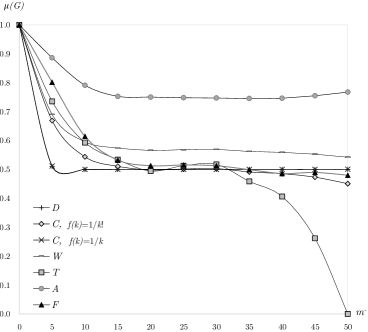
(a) The mean values of seven measures of partial balance

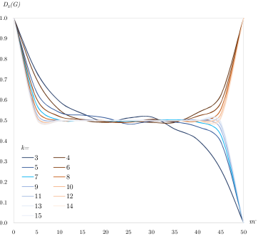
(b) The mean values of relative $k$-balance $D_{k}$

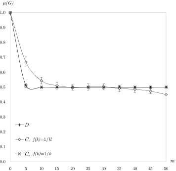
(c) The standard deviation of $D$ and $C$

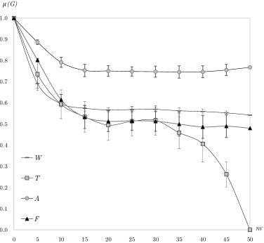
(d) The standard deviation of $W,T,A$ and $F$

Figure 1: Partial balance measured by different methods in Erdős-Rényi network with various number of negative edges (color version online)

Measures $D(G)$ and $C(G)$ with $f(k)=1/k$ are observed to tend to $0.5$ where $m^{-}>5$, not differentiating partial balance in graphs with a non-trivial number of negative edges. Given the typical distribution of cycles of different length, we expect $D(G)$ and $C(G)$ with $f(k)=1/k$ to be mostly determined by longer cycles that are much more frequent. For this particular graph, cycles with a length of 10 and above account for more than $96\%$ of the total cycles in the graph. Such long cycles tend to be balanced roughly half the time for almost all values of $m^{-}$ (for all the values within the range of $5\leq m^{-}\leq 45$ in the network considered here). The perfect overlap of data points for $D(G)$ and $C(G)$ with $f(k)=1/k$ in Figure 1 shows that using a linear rate of decay does not make a difference. One may think that if we use $D_{k}(G)$ which does not mix cycles of different length, it may circumvent the issues. However, subfigure (b) of Figure 1 demonstrating values of $D_{k}(G)$ for different cycle lengths shows the opposite. It shows not only does $D_{k}(G)$ not resolve the problems of lack of sensitivity and clustering around $0.5$, but it behaves unexpectedly with substantially different values based on the parity of $k$ when $m^{-}>35$. $C(G)$ weighted by $f(k)=1/k!$ and mostly determined by shorter cycles, decreases slower than $D(G)$ and then provides values close to $0.5$ for $m^{-}\geq 10$. $W(G)$ drops below $0.6$ for $m^{-}=10$ and then clusters around $0.55$ for $m^{-}>10$. $T(G)$ is the measure with a wide range of values symmetric to $m^{-}$. The single most striking observation to emerge is that $A(G)$ seems to have a completely different range of values, which we discuss further in Subsection 6.3. A steady linear decrease is observed from $F(G)$ for $m^{-}\leq 10$.

5.2 4-regular random networks of different orders

To investigate the impacts of graph order (number of nodes) and density on balance, we computed the measures for randomly generated 4-regular graphs with 50 percent negative edges. Intuitively we expect values to have low variation and no trends for similarly structured graphs of different orders. Figure 2 demonstrates the analysis in a setting where the degree of all the nodes remains constant, but the density ($4/n-1$) is decreasing in larger graphs. For each data point the average and standard deviation of 100 runs are reported. In each run, negative weights are randomly assigned to half of the edges in a fixed underlying 4-regular graph of order $n$.

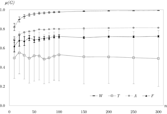
Figure 2: Partial balance measured by different methods in 50% negative 4-regular graphs of different orders $n$ and decreasing densities $4/n-1$

According to Figure 2, the four measures differ not only in the range of values, but also in their sensitivity to the graph order and density. First, $W(G)\rightarrow 1$ when $n\rightarrow\infty$ for larger graphs although the graphs are structurally similar, which goes against intuition. Clustered around $0.5$ is $T(G)$ which features a substantial standard deviation for 4-regular random graphs. Values of $A(G)$ are around $0.8$ and do not seem to change substantially when $n$ increases. $F(G)$ provides stationary values around $0.7$ when $n$ increases. While $\lambda(G)$ and $L(G)$ depend on the graph order and size, the relative constancy of $A(G)$ and $F(G)$ values suggest the normalized measures $A(G)$ and $F(G)$ are largely independent of the graph size and order, as our intuition expects. We further discuss the normalization of $A(G)$ and $F(G)$ in Subsection 6.3.

6 Analytical results on synthetic data

In this section, we analyze the capability of measuring partial balance in some families of specially structured graphs. Closed-form formulae for the measures in specially structured graphs are provided in Table 2. The two families of complete signed graphs that we investigate are as follows in 6.1 and 6.2.

6.1 Minimally unbalanced complete graphs with a single negative edge

The first family includes complete graphs with a single negative edge, denoted by ${K}_{n}^{a}$. Such graphs are only one edge away from a state of total balance. It is straight-forward to provide closed-form formulae for $\mu({K}_{n}^{a})$ as expressed in (30) – (36) in Appendix A.

Table 2: Balance in minimally and maximally unbalanced graphs ${K}_{n}^{a}$ (6.1) and ${K}_{n}^{c}$ (6.2)

$\mu(G)$	${K}_{n}^{a}$	${K}_{n}^{c}$
$D(G)$	$\sim 1-{2}/{n}$	$\sim\frac{1}{2}+(-1)^{n}e^{-2}$
$C(G),f(k)=1/k!$	$\sim 1-{1}/{n}$	$\sim\frac{1}{2}-\frac{3n\log n}{2^{n}}$
$D_{k}(G)$	$1-{2k}/{n(n-1)}$	$0,1$
$W(G)$	$\sim 1-{2}/{n}$	$\sim\frac{1+e^{2-2n}}{2}$
$A(G)$	$\sim 1-{4}/{n^{2}}$	$0$
$F(G)$	$1-{4}/{n(n-1)}$	$\frac{1}{n},\frac{1}{n-1}$

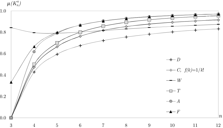
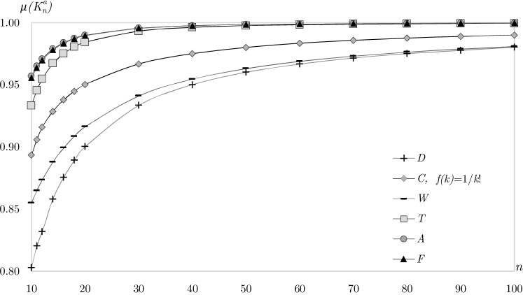
Figure 3: Partial balance measured by different methods for ${K}_{n}^{a}$ (6.1)

In ${K}_{n}^{a}$, intuitively we expect $\mu({K}_{n}^{a})$ to increase with $n$ and $\mu({K}_{n}^{a})\rightarrow 1$ as $n\rightarrow\infty$. We also expect the measure to detect the imbalance in ${K}_{3}^{a}$ (a triangle with one negative edge). Figure 3 demonstrates the behavior of different indices for complete graphs with one negative edge. $W({K}_{n}^{a})$ gives unreasonably large values for $n<5$. Except for $W({K}_{n}^{a})$, the measures are co-monotone over the given range of $n$.

6.2 Maximally unbalanced complete graphs with all-negative edges

The second family of specially structured graphs to analyze includes all-negative complete graphs denoted by ${K}_{n}^{c}$. The indices are calculated in (38) – (50) in Appendix A.

Intuitively, we expect $\mu({K}_{n}^{c})\rightarrow 0$ as $n\rightarrow\infty$. Figure 4 illustrates $D({K}_{n}^{c})$ oscillating around $0.5$ and $W({K}_{n}^{c}),C({K}_{n}^{c})\rightarrow 0.5$ as $n$ increases. We explain the oscillation of $D({K}_{n}^{c})$ in Appendix A. Clearly, measures $D(G)$, $C(G)$ and, $W(G)$ do no work well for the family of graphs considered here. Figure 4 shows that $F({K}_{n}^{c})\rightarrow 0$ as $n\rightarrow\infty$ as expected based on Table 2.

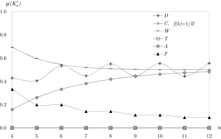
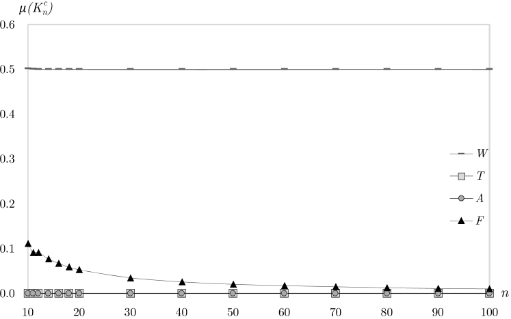
Figure 4: Partial balance measured by different methods for ${K}_{n}^{c}$ (6.2)

6.3 Normalization of the measures

It is worth mentioning that measures of partial balance may lead to different maximally unbalanced complete graphs. Based on $\lambda(G)$ and $L(G)$, ${K}_{n}^{c}$ represents the family of maximally unbalanced graphs, while it is merely one family among the maximally unbalanced graphs according to $T(G)$. Estrada and Benzi have found complete graphs comprised of one cycle of $n$ positive edges with the remaining pairs of nodes connected by negative edges to be a family of maximally unbalanced graphs based on $W(G)$ estrada_walk-based_2014 , while this argument is not supported by any other measures. As the signs of cycles in a graph are not independent, the structure of maximally unbalanced graphs under the cycle-based measures, $D(G)$ and $C(G)$, is not known.

A simple comparison of $L({K}_{n}^{c})$ (calculations provided in (47) in Appendix A) and the proposed upper bound $m/2=(n^{2}-n)/4$ reveals substantial gaps. These gaps equal $n/4$ for even $n$ and $(n-1)/4$ for odd $n$. This supports the previous discussions on looseness of $m/2$ as an upper bound for frustration index. As ${K}_{n}^{c}$ is maximally unbalanced under $L(G)$, $\lfloor m/2-(n-1)/4\rfloor$ can be used as a tight upper bound for normalizing the frustration index. This allows a modified version of normalized frustration index, denoted by $F^{\prime}(G)$ and defined in (18), to take the value zero for ${K}_{n}^{c}$.

$$F^{\prime}(G)=1-L(G)/\lfloor m/2-(n-1)/4\rfloor$$ (18)

Similarly, the upper bound, $\lambda_{\text{max}}(G)$, used to normalize algebraic conflict, is not tight for many graphs. For instance, in the Erdős-Rényi studied in Section 5 with $m=m^{-}$, the existence of an edge with $\overline{d}_{\text{max}}=9$ makes $\lambda_{\text{max}}(G)=8$, while $\lambda(G)=1.98$.

The two observations mentioned above suggest that tighter upper bounds can be used for normalization. However, the statistical analysis we use in Section 9 to evaluate balance in real networks is independent of the normalization method, so we do not pursue this question further now.

6.4 Expected values of the cycle-based measures

Relative $k$-balance, $D_{k}(G)$, is proved by El Maftouhi, Manoussakis and Megalakaki el_maftouhi_balance_2012 to tend to $0.5$ for Erdős-Rényi graphs such that the probability of an edge being negative is equal to $0.5$. Moreover, Giscard et al. discuss the probability distribution of $1-D_{k}(G)$. Their discussion is based on a model in which sign of any edge is negative with a fixed probability (Giscard2016, , Section 4.2). We use the same model to present some simple observations that appear not to have been noticed by previous authors advocating for the use of cycle-based measures. We are going to take a different approach from that of Giscard et al. and merely calculate the expected values of cycle-based measures in general, rather than the full distribution under additional assumptions. Note that, for an arbitrary graph, ${O_{k}^{+}}/{O_{k}}$ gives the probability that a randomly chosen $k$-cycle is balanced and is denoted by $B_{(k,q)}$.

Theorem 6.1.

Let $G$ be a graph and consider the sign function obtained by independently choosing each edge to be negative with probability $q$, and positive otherwise. Then

$$E(D_{k}(G)) =(1+{(1-2q)}^{k})/2$$ (19)

Proof 6.2.

Note that a cycle is balanced if and only if it has an even number of negative edges. Thus

$$E\left(\frac{O_{k}^{+}}{O_{k}}\right)=\sum\limits_{i\>\text{even}}{\binom{k}{i}}q^{i}(1-q)^{k-i}$$

(compare with (Giscard2016, , Eq. 4.1)). This simplifies to the stated formula (details of calculations are given in Appendix A).

Note that the expected values are independent of the graph structure and obtaining them does not require making any assumptions on the signs of cycles being independent random variables. As the signs of the edges are independent random variables, the expected value of $B_{(k,q)}$ can be obtained by summing on all cases having an even number of negative signs in the $k$-cycle.

Based on (19), $E(D_{k}(G))=1$ when $q=0$ and $E(D_{k}(G))=0.5$ when $q=0.5$ supporting our intuitive expectations. However, when $q=1$, $E(D_{k}(G))$ takes extremal values based on the parity of $k$ which is a major problem as previously observed in the subfigure (b) of Figure 1. It is clear to see that the parity of $k$ makes a substantial difference to $D_{k}(G)$ when a considerable proportion of edges are negative.

Theorem 6.3.

Let $G$ be a graph and consider the sign function obtained by independently choosing each edge to be negative with probability $q$, and positive otherwise. Then

$$E(D(G)) =\frac{1}{2}\frac{\sum\limits_{k=3}^{n}(1+{(1-2q)}^{k})(O_{k})}{\sum\limits_{k=3}^{n}O_{k}}$$ (20)

Proof 6.4.

The random variable ${O_{k}^{+}}$ can be written as ${O_{k}^{+}}=B_{(k,q)}.{O_{k}}$. Taking expected value from the two sides gives $E({O_{k}^{+}})={O_{k}}.E(B_{(k,q)})$ as $O_{k}$ is a constant for a fixed $k$. This completes the proof using the result from Theorem 6.1.

Note that the exponential decay of the factor $(1-2q)^{k}$ reduces the contribution for large $k$, and small values of $k$ will dominate for many graphs. For example, if $q=0.2$ the expression for $E(D(G))$ simplifies to

$$\frac{1}{2}+\frac{1}{2}\frac{\sum\limits_{k=3}^{n}{0.6}^{k}O_{k}}{\sum\limits_{k=3}^{n}O_{k}}.$$

For many graphs encountered in practice, $O_{k}$ will grow exponentially with $k$, but at a rate less than $1/0.6$, so the tail contribution will be small. Larger values of $q$ only make this effect more pronounced. Thus we expect that $E(D(G))$ will often be very close to $0.5$ in signed graphs with a reasonably large fraction of negative edges (we have already seen such a phenomenon in Subsection 5.1). A similar conclusion can be made for $C(G)$. This casts doubt on the usefulness of the measures that mix cycles of different length whether weighted or not.

While we have also observed many problems involving values of cycle-based measures on synthetic data in other parts of Sections 5 and 6, we will continue evaluating their axiomatic properties in Section 7 and then summarize the methodological findings in Section 8.

7 Axiomatic framework of evaluation

The results in Section 5 and Section 6 indicate that the choice of measure substantially affects the values of partial balance. Besides that, the lack of a standard measure calls for a framework of comparing different methods. Two different sets of axioms are suggested in norman_derivation_1972 , which characterize the measure $C(G)$ inside a smaller family (up to the choice of $f(k)$). Moreover, the theory of structural balance itself is axiomatized in schwartz_friend_2010 . However, to our knowledge, axioms for general measures of balance have never been developed. Here we provide the first set of axioms and desirable properties for measures of partial balance, in order to shed light on their characteristics and performance.

7.1 Axioms for measures of partial balance

We define a measure of partial balance to be a function $\mu$ taking each signed graph to an element of $[0,1]$. Worthy of mention is that some of these measures were originally defined as a measure of imbalance (algebraic conflict, frustration index and the original walk-based measure) calibrated at $0$ for completely balanced structures, so that some normalization was required, and perhaps our normalization choices can be improved on (see Subsection 6.3). As the choice of $m/2$ as the upper bound for normalizing the line index of balance was somewhat arbitrary, another normalized version of frustration index is defined in (21).

$$X(G)=1-L(G)/{m^{-}}$$ (21)

Before listing the axioms, we justify the need for an axiomatic evaluation of balance measures. As an attempt to understand the need for axiomatizing measures of balance, we introduce two unsophisticated and trivial measures that come to mind for measuring balance. The fraction of positive edges, denoted by $Y(G)$, is defined in (22) on the basis that all-positive signed graphs are balanced. Moreover, a binary measure of balance, denoted by $Z(G)$, is defined in (25). While $Y(G)$ and $Z(G)$ appear to be irrelevant, there is currently no reason not to use such measures.

$$Y(G)=m^{+}/m\quad$$ (22)

$$Z(G)=\left\{\begin{array}[]{ll}1&\mbox{if }$G \>$\mbox{is totally balanced}\\ 0&\mbox{if }$G \>$\mbox{is not balanced}\end{array}\right.$$ (25)

We consider the following notation for referring to basic operations on signed graphs:

$G^{g(X)}$ denotes signed graph $G$ switched by $g(X)$ (switched graph).
$G\oplus H$ denotes the disjoint union of two signed graphs $G$ and $H$ (disjoint union).
$G\ominus e$ denotes $G$ with $e$ deleted (removing an edge).
$G\ominus E^{*}$ denotes $G$ with minimum deletion edges removed (balanced transformation).
$G\oplus C^{+}_{3}$ denotes the disjoint union of graphs $G$ and a positive 3-cycle (adding a balanced 3-cycle).
$G\oplus C^{-}_{3}$ denotes the disjoint union of graphs $G$ and a negative 3-cycle (adding an unbalanced 3-cycle).
$e\in E^{*}$ denotes an edge in the minimum deletion set.
$G\ominus E^{*}\oplus e$ denotes the balanced transformation of a graph with an edge $e$ added to it.

We list the following axioms:

A1

$0\leq\mu(G)\leq 1$.

A2

$\mu(G)=1$ if and only if $G$ is balanced.

A3

If $\mu(G)\leq\mu(H)$, then $\mu(G)\leq\mu(G\oplus H)\leq\mu(H)$.

A4

$\mu(G^{g(X)})=\mu(G)$.

The justifications for such axioms are connected to very basic concepts in balance theory. We consider A1 essential in order to make meaningful comparisons between measures. Introducing the notion of partial balance, we argue that total balance, being the extreme case of partial balance, should be denoted by an extremal value as in A2. In A3, the argument is that the overall balance of two disjoint graphs is bounded between their individual balances. This also covers the basic requirement that the disjoint union of two copies of graph $G$ must have the same value of partial balance as $G$. Switching nodes should not change balance zaslavsky_matrices_2010 as in A4.

Table 3 shows how some measures fail on particular axioms. The results provide important insights into how some of the measures are not suitable for measuring partial balance. A more detailed discussion on the proof ideas and counterexamples related to Table 3 is provided in Appendix B.

Table 3: Different measures satisfying(✓) or failing(✗) axioms

	$D(G)$	$C(G)$	$W(G)$	$D_{k}(G)$	$A(G)$	$F(G)$	$X(G)$	$Y(G)$	$Z(G)$
A1	✓	✓	✓	✓	✓	✓	✓	✓	✓
A2	✓	✓	✓	✗	✗	✓	✓	✗	✓
A3	✓	✓	✓	✓	✗	✓	✓	✓	✓
A4	✓	✓	✓	✓	✓	✓	✗	✗	✓

7.2 Some other desirable properties

We also consider four desirable properties that formalize our expectations of a measure of partial balance. We do not consider the following as axioms in that they are based on adding or removing 3-cycles and edges which may bias the comparison in favor of cycle-based and frustration-based measures.

Positive and negative 3-cycles are very commonly used to explain the theory of structural balance which makes B1 and B2 obvious requirements. Removing an edge from a minimum deletion set, should not decrease balance as in B3. Finally, adding such an edge should not increase balance as in B4.

B1

If $\mu(G)\neq 1$, then $\mu(G\oplus C^{+}_{3})>\mu(G)$.

B2

If $\mu(G)\neq 0$, then $\mu(G\oplus C^{-}_{3})<\mu(G)$

B3

If $e\in E^{*}$, then $\mu(G\ominus e)\geq\mu(G)$.

B4

If $\mu(G)\neq 0$ and $\mu(G\ominus E^{*}\oplus e)\neq 1$, then $\mu(G\oplus e)\leq\mu(G)$.

Table 4 shows how some measures fail on particular desirable properties. It is worth mentioning that the evaluation in Tables 3–4 is somewhat independent of parametrization: for each strictly increasing function $h$ such that $h(0)=0$ and $h(1)=1$, the results in Tables 3–4 hold for $h(\mu(G))$. Proof ideas and counterexamples related to Table 4 is provided in Appendix B.

Table 4: Different measures satisfying(✓) or failing(✗) desirable properties

	$D(G)$	$C(G)$	$W(G)$	$D_{k}(G)$	$A(G)$	$F(G)$	$X(G)$	$Y(G)$	$Z(G)$
B1	✓	✓	✓	✗	✓	✓	✗	✗	✗
B2	✓	✓	✗	✗	✗	✗	✗	✗	✓
B3	✗	✗	✗	✗	✗	✓	✓	✗	✗
B4	✗	✗	✗	✗	✗	✓	✓	✗	✓

Another desirable property, which we have not formulated as a formal requirement owing to its vagueness, is that the measure takes on a wide range of values. For example, $D(G)$ and $C(G)$ tend rapidly to $0.5$ as $n$ increases which makes their interpretation and possibly comparison with other measures difficult. A possible way to formalize it would be expecting $\mu(G)$ to give $0$ and $1$ on each complete graph of order at least $3$, for some assignment of signs of edges. This condition would be satisfied by $T(G)$ and $A(G)$, as well as $F^{\prime}(G)$. However, $D(G),C(G)$ and $W(G)$ would not satisfy this condition due to the existence of balanced cycles and closed walks in complete signed graphs of general orders. Moreover, the very small standard deviation of $D(G)$, $C(G)$, and $W(G)$ makes statistical testing against the balance of reshuffled networks complicated. The measures $D(G)$, $C(G)$, and $W(G)$ also have shown some unexpected behaviors on various types of graphs discussed in Section 5 and Section 6.

8 Discussion on methodological findings

Taken together, the findings in Sections 5 – 7 give strong reason not to use cycle-based measures $D(G)$ and $C(G)$, regardless of the weights. The major issues with cycle-based measures $D(G)$ and $C(G)$ include the very small variance in randomly generated and reshuffled graphs, lack of sensitivity and clustering of values around 0.5 for graphs with a non-trivial number of negative edges. Recall the numerical analysis of synthetic data in Section 5, analytical results on the expected values of cycle-based measures in Subsection 6.4, and the numerical values which are difficult to interpret like the oscillation of $D(G)$ and values of $C(G)$ for ${K}_{n}^{c}$ graphs in Table 2 and Figure 4.

The relative $k$-balance which is ultimately from the same family of measures, seems to resolve some, but not all the problems discussed above. However, it fails on several axioms and desirable properties. It is easy to compute $D_{3}(G)$ based on closed walks of length 3 terzi_spectral_2011 and there are recent methods resolving the computational burden of computing $D_{k}(G)$ for general $k$ Giscard2016 ; giscard2016general . However, $D_{k>3}(G)$ cannot be used for cyclic graphs that do not have $k$-cycles. Besides, for networks with a large proportion of negative edges, the parity of $k$ substantially distorts the values of $D_{k}(G)$. Accepting all these shortcomings, one may use $D_{k}(G)$ when cycles of a particular length have a meaningful interpretation in the context of study.

Walk-based measures like $W(G)$ require a more systematic way of weighting to correct for the double-counting of closed walks with repeated edges. The shortcomings of $W(G)$ involving the weighting method and contribution of non-simple cycles are also discussed in Giscard2016 ; singh2017measuring . Recall that $W(G)\rightarrow 1$ in 4-regular graphs when we increase $n$ as in our discussion in Subsection 5.2. Besides, $W({K}_{n}^{c})\rightarrow 0.5$ as $n$ increases as discussed in Subsection 6.2. The commonly observed clustering of values near 0.5 may also present problems. Moreover, the model behind $W(G)$ is strange as signs of closed walks do not represent balance or imbalance. For these reasons we do not recommend $W(G)$ for future use.

The major weakness of the normalized algebraic conflict, $A(G)$, seems to be its incapability of evaluating the overall balance in graphs that have more than one connected component. Note that, some of the failures observed for $A(G)$ on axioms and desirable properties stem from its dependence on $\lambda(G)$ the smallest eigenvalue of the signed Laplacian matrix. $\lambda(G)$ might be determined by a component of the graph disconnected from other components and in turn not capturing the overall balance of the graph as a whole. For analysing graphs with just one cyclic connected component, one may use $A(G)$ while disregarding the acyclic components. However, if a graph has more than one cyclic connected component, using $A(G)$ or $\lambda(G)$ is similar to disregarding all but the most balanced connected component in the graph.

The three trivial measures, namely $X(G)$, $Y(G)$ and $Z(G)$, fail on various basic axioms and desirable properties in Tables 3 and 4, and also show a lack of sensitivity to the graph, making them inappropriate to be used as measures of balance.

Satisfying almost all the axioms and desirable properties, $F(G)$ seems to measure something different from what is obtained using all cycles or all $k$-cycles, and be worth pursuing in future. Note that, $L(G)$ equals the minimum number of unbalanced fundamental cycles iacono_determining_2010 ; suggesting a connection between the frustration and unbalanced cycles yet to be explored further. We recommend using $F(G)$ for all graphs as long as their size allows computing $L(G)$. Recently developed optimization models aref2017computing ; aref2016exact are shown to be capable of computing the frustration index in graphs of up to thousands of nodes and edges. For larger graphs, exact computation of $L(G)$ would be time consuming and it can be approximated using a nonzero optimality gap tolerance with the optimization models in aref2017computing ; aref2016exact . Alternatively, $A(G)$ and $D_{k}(G)$ seem to be the other options. Depending on the type of the graph, $k$-cycles might not necessarily capture global structural properties. For instance, this would make $D_{3}(G)$ an improper choice for some specific graphs like sparse 4-regular graphs (as in Subsection 5.2), square grids, and sparse graphs with a small number of 3-cycles. Similarly, $A(G)$ is not suitable for graphs that have more than one connected component (including many sparse graphs).

Notes on previous work

In the literature, balance theory is widely used on directed signed graphs. It seems that this approach is questionable in two ways. First, it neglects the fact that many edges in signed digraphs are not reciprocated. Bearing that in mind, investigating balance theory in signed digraphs deals with conflict avoidance when one actor in such a relationship may not necessarily be aware of good will or ill will on the part of other actors. This would make studying balance in directed networks analogous to studying how people avoid potential conflict resulting from potentially unknown ties. Secondly, balance theory does not make use of the directionality of ties and the concepts of sending and receiving positive and negative links.

Leskovec, Huttenlocher and Kleinberg compare the reliability of predictions made by competing theories of social structure: balance theory and status theory (a theory that explicitly includes direction and gives quite different predictions) leskovec_signed_2010 . The consistency of these theories with observations is investigated through large signed directed networks such as Epinions, Slashdot, and Wikipedia. The results suggest that status theory predicts accurately most of the time while predictions made by balance theory are incorrect half of the time. This supports the inefficacy of balance theory for structural analysis of signed digraphs. For another comparison of the theories on signed networks, one may refer to a study of 8 theories to explain signed tie formation between students yap_why_2015 .

In a parallel line of research on network structural analysis, researchers differentiate between classical balance theory and structural balance specifically in the way that the latter is directional bonacich_introduction_2012 . They consider another setting for defining balance where absence of ties implies negative relationships. This assumption makes the theory limited to complete signed digraphs. Accordingly, 64 possible structural configurations emerge for three nodes. These configurations can be reduced to 16 classes of triads, referred to as 16 MAN triad census, based on the number of Mutual, Asymmetric, and Null relationships they contain. There are only 2 out of 16 classes that are considered balanced. New definitions are suggested by researchers in order to make balance theory work in a directional context. According to Prell prell_social_2012 , there is a second, a third, and a fourth definition of permissible triads allowing for 3, 7, and 9 classes of all 16 MAN triads. However, there have been many instances of findings in conflict with expectations prell_social_2012 .

Apart from directionality, the interpretation of balance measures is very important. Numerous studies have compared balance measures with their extremal values and found that signed networks are far from balanced, for example estrada_walk-based_2014 . However, with such a strict criterion, we must be careful not to look for properties that are almost impossible to satisfy. A much more systematic approach is to compare values of partial balance in the signed graphs in question to the corresponding values for reshuffled graphs Szell_multi ; Szell_measure as we have done in Section 9.

So far we formalized the notion of partial balance and compared various measures of balance based on their values in different graphs where the underlying structure was not important. We also evaluated the measures based on their axiomatic properties and ruled out the measures that we could not justify. In the next section, we focus on exploring real signed graphs based on the justified methods.

9 Results on real signed networks

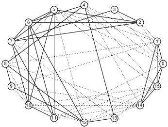
(a) Highland tribes network (G1), a signed network of 16 tribes of the Eastern Central Highlands of New Guinea read_cultures_1954

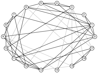
(b) Monastery interactions network (G2) of 18 New England novitiates inferred from the integration of all positive and negative relationships sampson_novitiate_1968

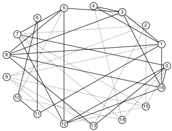
(c) Fraternity preferences network (G3) of 17 boys living in a pseudo-dormitory inferred from ranking data of the last week in newcomb_acquaintance_1961

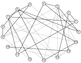
(d) College preferences network (G4) of 17 girls at an Eastern college inferred from ranking data of house B in lemann_group_1952

Figure 5: Four small signed networks visualized where dotted lines represent negative edges and solid lines represent positive edges

In this section, we analyze partial balance for a range of signed networks inferred from datasets of positive and negative interactions and preferences. Read’s dataset for New Guinean highland tribes read_cultures_1954 is demonstrated as a signed graph (G1) in Figure 5(a), where dotted lines represent negative edges and solid lines represent positive edges. The fourth time window of Sampson’s dataset for monastery interactions sampson_novitiate_1968 (G2) is drawn in Figure 5(b). We also consider datasets of students’ choice and rejection (G3 and G4) newcomb_acquaintance_1961 ; lemann_group_1952 as demonstrated in Figure 5(c) and Figure 5(d). The last three are converted to undirected signed graphs by considering mutually agreed relations. A further explanation on the details of inferring signed graphs from the choice and rejection data is provided in Appendix C.

A larger signed network (G5) is inferred by neal_backbone_2014 through implementing a stochastic degree sequence model on Fowler’s data on Senate bill co-sponsorship fowler_legislative_2006 . Besides the signed social network datasets, large scale biological networks can be analysed as signed graphs. There are relatively large signed biological networks analysed by dasgupta_algorithmic_2007 and iacono_determining_2010 from a balance viewpoint under a different terminology where monotonocity is the equivalent for balance. The two gene regulatory networks we consider are related to two organisms: a eukaryote (the yeast Saccharomyces cerevisiae) and a bacterium (Escherichia coli). Graphs G6 and G7 represent the gene regulatory networks of Saccharomyces cerevisiae Costanzo2001yeast and Escherichia coli salgado2006ecoli respectively. Note that, the densities of these networks are much smaller than the other networks introduced above. In gene regulatory networks, nodes represent genes. Positive and negative edges represent activating connections and inhibiting connections respectively. Figure 6 shows the bill co-sponsorship network as well as biological signed networks. The color of edges correspond to the signs on the edges (green for $+1$ and red for $-1$). For more details on the biological datasets, one may refer to iacono_determining_2010 .

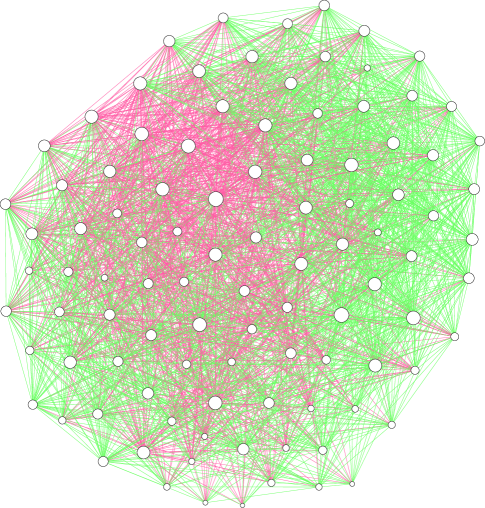
(a) The bill co-sponsorship network (G5) of senators neal_backbone_2014

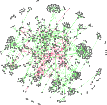
(b) The gene regulatory network (G6) of Saccharomyces cerevisiae Costanzo2001yeast

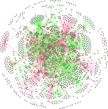
(c) The gene regulatory network (G7) of the Escherichia coli salgado2006ecoli

Figure 6: Three larger signed datasets illustrated as signed graphs in which red lines represent negative edges and green lines represent positive edges (color version online)

As Figure 6 shows, graphs G6 and G7 have more than one connected component. Besides the giant component, there are a number of small components that we discard in order to use $A(G)$ and $\lambda(G)$. Note that, this procedure does not change $T(G)$ and $L(G)$ as the small components are all acyclic. The values of $(n,m,m^{-})$ for giant components of G6 and G7 are $(664,1064,220)$ and $(1376,3150,1302)$ respectively.

The results are shown in Table 5. Although neither of the networks is completely balanced, the small values of $L(G)$ suggest that removal of relatively few edges makes the networks completely balanced. Table 5 also provides a comparison of partial balance between different datasets of similar sizes. In this regard, it is essential to know that the choice of measure can make a substantial difference. For instance among G1–G4, under $T(G)$, G1 and G3 are respectively the most and the least partially balanced networks. However, if we choose $A(G)$ as the measure, G1 and G3 would be the least and the most partially balanced networks respectively. This confirms our previous discussions on how choosing a different measure can substantially change the results and helps to clarify some of the conflicting observations in the literature facchetti_computing_2011 ; kunegis_applications_2014 and estrada_walk-based_2014 , as previously discussed in Section 8.

Table 5: Partial balance computer for signed graphs (G1–7) and reshuffled graphs

Graph:$(n,m,m^{-})$	Density		$T$	$A$	$F$	$\lambda$	$L$
G1: (16, 58, 29)	0.483	$\mu(G)$	0.87	0.88	0.76	1.04	7
		$\text{mean}(\mu(G_{r}))$	0.50	0.76	0.49	2.08	14.65
		$\text{SD}(\mu(G_{r}))$	0.06	0.02	0.05	0.20	1.38
		Z-score	6.04	5.13	5.54	$-5.13$	$-5.54$
G2: (18, 49, 12)	0.320	$\mu(G)$	0.86	0.88	0.80	0.75	5
		$\text{mean}(\mu(G_{r}))$	0.55	0.79	0.60	1.36	9.71
		$\text{SD}(\mu(G_{r}))$	0.09	0.03	0.05	0.18	1.17
		Z-score	3.34	3.37	4.03	$-3.37$	$-4.03$
G3:(17, 40, 17)	0.294	$\mu(G)$	0.78	0.90	0.80	0.50	4
		$\text{mean}(\mu(G_{r}))$	0.49	0.82	0.62	0.89	7.53
		$\text{SD}(\mu(G_{r}))$	0.11	0.06	0.06	0.30	1.24
		Z-score	2.64	1.32	2.85	$-1.32$	$-2.85$
G4: (17, 36, 16)	0.265	$\mu(G)$	0.79	0.88	0.67	0.71	6
		$\text{mean}(\mu(G_{r}))$	0.49	0.87	0.64	0.79	6.48
		$\text{SD}(\mu(G_{r}))$	0.14	0.03	0.06	0.17	1.08
		Z-score	2.16	0.50	0.45	$-0.50$	$-0.45$
G5: (100, 2461, 1047)	0.497	$\mu(G)$	0.86	0.87	0.73	8.92	331
		$\text{mean}(\mu(G_{r}))$	0.50	0.75	0.22	17.46	965.6
		$\text{SD}(\mu(G_{r}))$	0.00	0.00	0.01	0.02	9.08
		Z-score	118.5	387.8	69.89	$-387.8$	$-69.89$
G6:(690, 1080, 220)	0.005	$\mu(G)$	0.54	1.00	0.92	0.02	41
		$\text{mean}(\mu(G_{r}))$	0.58	1.00	0.77	0.02	124.3
		$\text{SD}(\mu(G_{r}))$	0.07	0.00	0.01	0.00	4.97
		Z-score	$-0.48$	8.61	16.75	$-8.61$	$-16.75$
G7:(1461, 3215, 1336)	0.003	$\mu(G)$	0.50	1.00	0.77	0.06	371
		$\text{mean}(\mu(G_{r}))$	0.50	1.00	0.59	0.06	653.4
		$\text{SD}(\mu(G_{r}))$	0.02	0.00	0.00	0.00	7.71
		Z-score	$-0.33$	3.11	36.64	$-3.11$	$-36.64$

In Table 5, the mean and standard deviation of measures for the reshuffled graphs $(G_{r})$, denoted by $\text{mean}(\mu(G_{r}))$ and $\text{SD}(\mu(G_{r}))$, are also provided for comparison. We implement a very basic statistical analysis as in Szell_multi ; Szell_measure using $\text{mean}(\mu(G_{r}))$ and $\text{SD}(\mu(G_{r}))$ of 500 reshuffled graphs. Reshuffling the signs on the edges 500 times, we obtain two parameters of balance distribution for the fixed underlying structure. For measures of balance, Z-scores are calculated based on Equation (26).

$$Z=\frac{\mu(G)-\text{mean}(\mu(G_{r}))}{\text{SD}(\mu(G_{r}))}$$ (26)

The Z-score shows how far the balance is with regards to balance distribution of the underlying structure. Positive values of Z-score for $T(G)$, $A(G)$, and $F(G)$ can be interpreted as existence of more partial balance than the average random level of balance.

It is worth pointing out that the statistical analysis we have implemented is independent of the normalization method used in $A(G)$ and $F(G)$. The two right columns of 5 provide $\lambda(G)$ and $L(G)$ alongside their associated Z-scores.

The Z-scores show that as measured by the frustration index and algebraic conflict, signed networks G1–G7 exhibit a level of partial (but not total) balance beyond what is expected by chance. Based on these two measures, the level of partial balance is high for graphs G1, G2, G5, G6, and G7 while the numerical results for G3 and G4 do not allow a conclusive interpretation. It indicates that most of the real signed networks investigated are relatively consistent with the theory of structural balance. However, the Z-scores obtained based on the triangle index for G6–G7 show totally different results. Note that G6 and G7 are relatively sparse graphs which only have 70 and 1052 triangles. This may explain the difference between Z-scores of $T(G)$ and that of other measures. The numerical results using the algebraic conflict and frustration index support previous observations of real-world networks’ closeness to balance facchetti_computing_2011 ; kunegis_applications_2014 .

10 Conclusion and Future research

In this study, we started by discussing balance in signed networks in Sections 2 and 3 and introduced the notion of partial balance. We discussed different ways to measure partial balance in Section 4 and provided some observations on synthetic data in Sections 5 and 6. After gaining an understanding of the behaviour of different measures, basic axioms and desirable properties were used in Section 7 to rule out the measures that cannot be justified.

We have discussed various methodologies and how they have led to conflicting observations in the literature in Section 8. Taking axiomatic properties of the measures into account, using the common cycle-based measures denoted by $D(G)$ and $C(G)$ and the walk-based measure $W(G)$ is not recommended. $D_{k}(G)$ and $A(G)$ may introduce some problems, but overall using them seems to be more appropriate compared to $D(G)$, $C(G)$ and $W(G)$. The observations on synthetic data taken together with the axiomatic properties, recommend $F(G)$ as the best overall measure of partial balance. However, considering the difficulty of computing the exact value of $L(G)$ for very large graphs, one may approximate it using a nonzero optimality gap tolerance with the optimization models in aref2017computing ; aref2016exact . Alternatively, $A(G)$ and $D_{k}(G)$ seem to be the other options accepting their potential shortcomings.

Using the three measures $F(G)$, $T(G)$, and $A(G)$, each representing a family of measures, we compared balance in real signed graphs and analogous reshuffled graphs having the same structure in Section 9. Table 5 provides this comparison showing that different results are obtained under different measures.

Returning to the questions posed at the beginning of this paper, it is now possible to state that under the frustration index and algebraic conflict many signed networks exhibit a level of partial (but not total) balance beyond that expected by chance. However, the numerical results in Table 5 show that the level of balance observed using the triangle index can be totally different. One of the more significant findings to emerge from this study is that methods suggested for measuring balance may have different context and may require some justification before being interpreted based on their values. The present study confirms that some measures of partial balance cannot be taken as a reliable static measure to be used for analyzing network dynamics.

Although a numerical part of the current study is based on signed networks with less than a few thousand nodes, the analytical findings that were not restricted to a particular size suggest the inefficacy of some methods for analyzing larger networks as well.

One gap in this study is that we avoid using structural balance theory for analyzing directed networks, making directed signed networks like Epinions, Slashdot, and Wikipedia Elections leskovec_signed_2010 ; estrada_walk-based_2014 ; Giscard2016 datasets untested by our approach. However, see our discussion in Section 8.

The findings of this study have a number of important implications for future investigation. Although this study focuses on partial balance, the findings may well have a bearing on link prediction and clustering in signed networks Gallier16 . Some other theoretical topics of interest in signed networks are network dynamics tan_evolutionary_2016 and opinion dynamics li_voter_2015 . Effective methods of signed network structural analysis can contribute to these topics as well. From a practical viewpoint, international relations is a crucial area to implement signed network structural analysis. Having an efficient measure of partial balance in hand, international relations can be investigated in terms of evaluation of partial balance over time for networks of states.

Appendix A Details of calculations

In order to simplify the sum $E(D_{k}(G))=\sum\limits_{i\>\text{even}}{\binom{k}{i}}q^{i}(1-q)^{k-i}$, one may add the two following equations and divide the result by 2:

$$\sum\limits_{i}{\binom{k}{i}}q^{i}(1-q)^{k-i} =(q+(1-q))^{k}$$ (27)

$$\sum\limits_{i}{\binom{k}{i}}(-q)^{i}(1-q)^{k-i} =(-q+(1-q))^{k}$$ (28)

In ${K}_{n}^{a}$, a $k$-cycle is specified by choosing $k$ vertices in some order, then correcting for the overcounting by dividing by $2$ (the possible directions) and $k$ (the number of starting points, namely the length of the cycle). If the unique negative edge is required to belong to the cycle, by orienting this in a fixed way we need choose only $k-2$ further elements in order, and no overcounting occurs. The numbers of negative cycles and total cycles are as follows.

$$\sum_{k=3}^{n}O_{k}^{-}=\sum_{k=3}^{n}\frac{(n-2)!}{(n-k)!},\quad\sum_{k=3}^{n}O_{k}=\sum_{k=3}^{n}\frac{n!}{2k(n-k)!}$$ (29)

Asymptotic approximations for these sums can be obtained by introducing the exponential generating function. For example, letting

$$a_{n}=\sum_{1\leq k\leq n}\frac{n!}{(n-k)!k}$$

we have

$$\sum_{n\geq 0}\frac{a_{n}}{n!}x^{n}=\sum_{n,k}\sum_{k\leq n}\frac{n!}{(n-k)!k}x^{n}=\sum_{k\geq 1}\frac{1}{k}\sum_{n\geq k}\frac{1}{(n-k)!}x^{n}=\sum_{k\geq 1}\frac{x^{k}}{k}\sum_{m\geq 0}\frac{1}{m!}x^{m}=e^{x}\log\left(\frac{1}{1-x}\right).$$

Similarly we obtain

$$\sum_{n\geq 0}\sum_{k\geq 0}\frac{1}{(n-k)!}x^{n}=\frac{e^{x}}{1-x}.$$

Standard singularity analysis methods flajolet2009analytic show the denominator of the expression for $D(K^{a}_{n})$ to be asymptotic to $(n-1)!e/2$ while the number of negative cycles is asymptotic to $(n-2)!e$. Similarly the weighted sum defining $C(K^{a}_{n})$, where we choose $f(k)=1/k!$, can be expressed using the ordinary generating function, which for the denominator turns out to be

$$\frac{1}{1-x}\log\left(\frac{1-2x}{1-x}\right).$$

Again, singularity analysis techniques yield an approximation $2^{n}/n$. The numerator is easier, and asymptotic to $2^{n}/(n^{2}-n)$. This yields the result.

The unsigned adjacency matrix $|\textbf{A}|$ of the complete graph has the form $\textbf{E}-\textbf{I}$ where E is the matrix of all $1$’s. The latter matrix has rank 1 and nonzero eigenvalue $n$. Thus $|\textbf{A}|_{({K}_{n}^{a})}$ has eigenvalues $n-1$ (with multiplicity 1) and $-1$ (with multiplicity $n-1$). The matrix $\textbf{A}_{({K}_{n}^{a})}$ has a similar form and we can guess eigenvectors of the form $(-1,1,0,\dots,0)$ and $(a,a,1,1,\dots,1)$. Then $a$ satisfies a quadratic $2a^{2}+(n-3)a-(n-2)=0$. Solving for $a$ and the corresponding eigenvalues, we obtain eigenvalues $(n-4\pm\sqrt{(n-2)(n+6)})/2,1,-1$ (with multiplicity $n-3$)).

This yields

$$K{({K}_{n}^{a})}=\frac{(n-3)e^{-1}+e+e^{\frac{n-4-\sqrt{(n-2)(n+6)}}{2}}+e^{\frac{n-4+\sqrt{(n-2)(n+6)}}{2}}}{(n-1)e^{-1}+e^{n-1}}$$

which results in $W({K}_{n}^{a})\sim\frac{1+e^{-4/n}}{2}$.

Furthermore, since every node of $K_{n}$ has degree $n-1$, the eigenvalues of $\textbf{L}:=(n-1)\textbf{I}-\textbf{A}$ are precisely of the form $n-1-\lambda$ where $\lambda$ is an eigenvalue of A.

Measures of partial balance for ${K}_{n}^{a}$ can therefore be expressed by the formulae (30) – (36):

$$D({K}_{n}^{a})=1-\frac{\sum_{k=3}^{n}\frac{(n-2)!}{(n-k)!}}{\sum_{k=3}^{n}\frac{n!}{2k(n-k)!}}\sim 1-\frac{2}{n}$$ (30)

$$C({K}_{n}^{a})=1-\frac{\sum_{k=3}^{n}\frac{(n-2)!}{(n-k)!k!}}{\sum_{k=3}^{n}\frac{n!}{2k(n-k)!k!}}\sim 1-\frac{1}{n}$$ (31)

$$D_{k}({K}_{n}^{a})=1-\frac{\frac{(n-2)!}{(n-k)!}}{\frac{n!}{2k(n-k)!}}=1-\frac{2k}{n(n-1)}\sim 1-\frac{2k}{n^{2}}$$ (32)

$$W({K}_{n}^{a})\sim\frac{1+e^{-4/n}}{2}\sim 1-\frac{2}{n}$$ (33)

$$\lambda({K}_{n}^{a})=n-1-(n-4+\sqrt{(n-2)(n+6)})/2=(n+2-\sqrt{(n-2)(n+6)})/2$$ (34)

$$A({K}_{n}^{a})=1-\frac{n+2-\sqrt{(n-2)(n+6)}}{2n-4}\sim 1-\frac{4}{n^{2}}$$ (35)

$$F({K}_{n}^{a})=1-\frac{2}{n(n-1)/2}=1-\frac{4}{n(n-1)}\sim 1-\frac{4}{n^{2}}$$ (36)

In ${K}_{n}^{c}$, all cycles of odd length are unbalanced and all cycles of even length are balanced. Therefore:

$$\sum_{k=3}^{n}O_{k}^{+}=\sum_{\textnormal{even}}^{n}\frac{n!}{2k(n-k)!}$$ (37)

It follows that $D_{k}({K}_{n}^{c})$ equals 0 for odd $k$ and 1 for even $k$. Based on maximality of $\lambda(G)$ in ${K}_{n}^{c}$, $A({K}_{n}^{c})=0$.

Using the above generating function techniques we obtain that the numerator of $D(K^{c}_{n})$ is asymptotic to $(n-1)!(e+(-1)^{n}e^{-1})/4$. The denominator we know from above is asymptotic to $(n-1)!e/2$. This yields $D(K^{c}_{n})\sim 1/2+(-1)^{n}e^{-2}$. Note that $e^{-2}\approx 0.135$ and this explains the oscillation in Figure 4. Similarly we obtain results for $C(K^{c}_{n})$.

$|\textbf{A}|_{({K}_{n}^{c})}$ has eigenvalues $n-1$ (with multiplicity 1) and $-1$ (with multiplicity $n-1$). The matrix $\textbf{A}_{({K}_{n}^{c})}$ has a similar form and the corresponding eigenvalues would be $1-n$ (with multiplicity 1) and $1$ (with multiplicity $n-1$). This yields $K{({K}_{n}^{c})}=\frac{(n-1)e^{1}+e^{1-n}}{(n-1)e^{-1}+e^{n-1}}$ which results in $W({K}_{n}^{c})\sim\frac{1+e^{2-2n}}{2}$.

Moreover, a closed-form formula for $L({K}_{n}^{c})$ can be expressed based on a maximum cut which gives a function of $n$ equal to an upper bound of the frustration index under a different name in abelson_symbolic_1958 . Measures of partial balance for ${K}_{n}^{c}$ can be expressed via the closed-form formulae as stated in (38) – (50):

$$D({K}_{n}^{c})=\frac{\sum_{\textnormal{$k$ even}}^{n}\frac{n!}{2k(n-k)!}}{\sum_{k=3}^{n}\frac{n!}{2k(n-k)!}}\sim\frac{1}{2}+(-1)^{n}e^{-2}$$ (38)

$$C({K}_{n}^{c})=\frac{\sum_{\textnormal{$k$ even}}^{n}\frac{n!}{2k(n-k)!k!}}{\sum_{k=3}^{n}\frac{n!}{2k(n-k)!k!}}\sim\frac{1}{2}-\frac{3n\log n}{2^{n}}$$ (39)

$$D_{k}({K}_{n}^{c})=\left\{\begin{array}[]{ll}1&\mbox{if }k\ \text{is even}\\ 0&\mbox{if }k\ \text{is odd}\end{array}\right.$$ (42)

$$W({K}_{n}^{c})\sim\frac{1+e^{2-2n}}{2}$$ (43)

$$\lambda({K}_{n}^{c})=\lambda_{\text{max}}=\overline{d}_{\text{max}}-1=n-2$$ (44)

$$L({K}_{n}^{c})=\left\{\begin{array}[]{ll}({n^{2}-2n})/{4}&\mbox{if }n\ \text{is even}\\ ({n^{2}-2n+1})/{4}&\mbox{if }n\ \text{is odd}\end{array}\right.$$ (47)

$$F({K}_{n}^{c})=\left\{\begin{array}[]{ll}1-\frac{n(n-2)/4}{n(n-1)/4}=\frac{1}{n-1}&\mbox{if }n\ \text{is even}\\ 1-\frac{(n-1)(n-1)/4}{n(n-1)/4}=\frac{1}{n}&\mbox{if }n\ \text{is odd}\end{array}\right.$$ (50)

Our calculations for $L({K}_{n}^{c})$ show that the upper bound suggested for the frustration index in iacono_determining_2010 is incorrect.

Appendix B Counterexamples and proof ideas for the axioms and desirable properties

Axioms:

Axiom 1 holds in all the measures introduced due to the systematic normalization implemented.

$D_{k}(G)$, $A(G)$, and $Y(G)$ do not satisfy Axiom 2. All $k$-cycles being balanced, $D_{k}(G)$ fails to detect the imbalance in graphs with unbalanced cycles of different length. $A(G\oplus C^{+})=1$ for unbalanced graphs which makes $A(G)$ fail Axiom 2. $Y(G)$ fails on detecting balance in completely bi-polar signed graphs that are indeed balanced.

As long as $\mu(G\oplus H)$ can be written in the form of $(a+c)/(b+d)$ where $\mu(G)=a/b$ and $\mu(H)=c/d$, $\mu$ satisfies Axiom 3. So all the measures considered satisfy Axiom 3, except for $A(G)$. In case of $\lambda(G)<\lambda(H)$ and $\lambda_{\text{max}}(G)<\lambda_{\text{max}}(H)$, $A(G\oplus H)=1-\frac{\lambda(G)}{\lambda_{\text{max}}(H)}>A(H)$ which shows that $A(G)$ fails Axiom 3.

The sign of cycles (closed walks), the Laplacian eigenvalues Belardo2016 , and the frustration index zaslavsky_matrices_2010 will not change by applying the switching function introduced in (9). Therefore, Axiom 4 holds for all the measures discussed except for $X(G)$ and $Y(G)$ because they depend on $m^{-}$, which changes in switching.

Desirable properties:

Clearly in B1, $C^{+}_{3}$ contributes positively to $D(G)$ and $C(G)$, whereas for $D_{k}(G)$ it depends on $k$ which makes it fail B1. As $W(C^{+}_{3})$ equals 1, $\operatorname{Tr}(e^{\textbf{A}})/\operatorname{Tr}(e^{|\textbf{A}|})$ would be added by equal terms in both the numerator and denominator leading to $W(G)$ satisfying B1. $A(G)$ satisfies B1 because $A(G\oplus C^{+}_{3})=1$. As $m$ increases by 3, $F(G)$ satisfies B1. The dependency of $X(G)$ and $Y(G)$ on $m^{-}$ and incapability of the binary measure, $Z(G)$, in providing values between 0 and 1 make them fail B1.

$C^{-}_{3}$ adds only to the denominators of $D(G)$ and $C(G)$, whereas for $D_{k}(G)$ it depends on $k$ which makes it fail B2. Following the addition of a negative 3-cycle, $W(G)$ is observed to increase resulting in its failure in B2 (for example, take $G=K_{5}$ with single negative edge, and $C^{-}_{3}$ having a single negative edge). As $A(G)\neq 0$ and $A(C^{-}_{3})=0$, the value of $A(G\oplus C^{-}_{3})$ does not change when a negative 3-cycle is added. Therefore, it fails B2. Moreover, $F(G)$ fails B2 whenever $L(G)\geq m/3$ as observed in a family of graphs in Subsection 6.2. However, $F^{\prime}(G)$ introduced in Eq. 18 which only differs in normalization, satisfies this desirable property. The measures $X(G)$ and $Y(G)$ fail B2, but the binary measure, $Z(G)$, satisfies it.

All the cycle-based measures, namely $D(G),C(G)$, and $D_{3}(G)$ fail B3 (for example, take $G=K_{4}$ with two symmetrically located negative edges). $W(G)$ is also observed to fail B3 (for instance, take $G$ as the disjoint union of a 3-cycle and a 5-cycle each having 1 negative edge). It is known that $\lambda(G\ominus e)\leq\lambda(G)$ Belardo2016 . However in some cases where $\lambda_{\text{max}}(G\ominus e)<\lambda_{\text{max}}(G)$ counterexamples are found showing $A(G)$ fails on B3 (consider a graph with $n=8,m^{+}=10,m^{-}=3,\min{|E^{*}|}=3$ in which $\lambda_{\text{max}}(G)=6$ and $\lambda_{\text{max}}(G\ominus e)=3$). $Y(G)$ and $Z(G)$ fail B3. Moreover, $F(G)$ satisfies B3 because $L(G\ominus e)=L(G)-1$.

The cycle-based measures and $W(G)$ do not satisfy B4. For $D_{3}(G)$, we tested a graph with $n=7,m=15,|E^{*}|=3$ and we observed $D_{3}(G\oplus e)>D_{3}(G)$. According to Belardo and Zhou, $\lambda(G\oplus e)\geq\lambda(G)$ Belardo2016 . However in some cases where $\lambda_{\text{max}}(G\oplus e)>\lambda_{\text{max}}(G)$ counterexamples are found showing $A(G)$ fails on B4. counterexamples showing $D(G),C(G),W(G)$, and $A(G)$ fail B4, are similar to that of B3. Moreover, $F(G)$ satisfies B4 as do $X(G)$ and $Z(G)$, while $Y(G)$ fails B4 when $e$ is positive.

Appendix C Inferring undirected signed graphs

Sampson collected different sociometric rankings from a group of 18 monks at different times sampson_novitiate_1968 . The data provided includes rankings on like, dislike, esteem, disesteem, positive influence, negative influence, praise, and blame. We have considered all positive and negative rankings. Then only the reciprocated relations with similar signs are considered to infer an undirected signed edge between two monks (see doreian_partitioning_2009 and how the authors inferred a directed signed graph in their Table 5 by summing the influence, esteem and respect relations).

Newcomb reported rankings made by 17 men living in a pseudo-dormitory newcomb_acquaintance_1961 . We used the ranking data of the last week which includes complete ranks from 1 to 17 gathered from each man. As the gathered data is related to complete ranking, we considered ranks 1-5 as one-directional positive relations and 12-17 as one-directional negative relations. Then only the reciprocated relations with similar signs are considered to infer an undirected signed edge between two men (see doreian_partitioning_2009 and how the authors converted the top three and bottom three ranks to a directed signed edges in their Fig. 4.).

Lemann and Solomon collected ranking data based on multiple criteria from female students living in off-campus dormitories lemann_group_1952 . We used the data for house B which is resulted by integrating top and bottom three rankings for multiple criteria. As the gathered data itself is related to top and bottom rankings, we considered all the ranks as one-directional signed relations. Then only the reciprocated relations with similar signs are considered to infer an undirected signed edge between two women (see doreian_multiple_2008 and how the author inferred a directed signed graph in their Fig. 5 from the data for house B.).

References

- [1] Robert P. Abelson and Milton J. Rosenberg. Symbolic psycho-logic: A model of attitudinal cognition. Behavioral Science, 3(1):1–13, 1958.
- [2] Belmannu Devadas Acharya. Spectral criterion for cycle balance in networks. Journal of Graph Theory, 4(1):1–11, 1980.
- [3] Jin Akiyama, David Avis, Vasek Chvátal, and Hiroshi Era. Balancing signed graphs. Discrete Applied Mathematics, 3(4):227–233, 1981.
- [4] Samin Aref, Andrew J Mason, and Mark C Wilson. An exact method for computing the frustration index in signed networks using binary programming. Preprint arXiv:1611.09030, 2016.
- [5] Samin Aref, Andrew J Mason, and Mark C Wilson. Computing the line index of balance using integer programming optimisation. In Boris Goldengorin, editor, Optimization Problems in Graph Theory, pages 67–86. Springer, 2018.
- [6] Francesco Belardo. Balancedness and the least eigenvalue of Laplacian of signed graphs. Linear Algebra and its Applications, 446:133 – 147, 2014.
- [7] Francesco Belardo and Yue Zhou. Signed graphs with extremal least Laplacian eigenvalue. Linear Algebra and its Applications, 497:167 – 180, 2016.
- [8] Etienne Birmelé, Rui Ferreira, Roberto Grossi, Andrea Marino, Nadia Pisanti, Romeo Rizzi, and Gustavo Sacomoto. Optimal listing of cycles and st-paths in undirected graphs. In Sanjeev Khanna, editor, Proceedings of the Twenty-fourth Annual ACM-SIAM Symposium on Discrete Algorithms, SODA ’13, pages 1884–1896, Philadelphia, PA, USA, 2013. Society for Industrial and Applied Mathematics.
- [9] Phillip Bonacich. Introduction to mathematical sociology. Princeton University Press, Princeton, 2012.
- [10] Qing Cai, Maoguo Gong, Lijia Ma, Shanfeng Wang, Licheng Jiao, and Haifeng Du. A particle swarm optimization approach for handling network social balance problem. In Shigeru Obayashi, Carlo Poloni, and Tadahiko Murata, editors, 2015 IEEE Congress on Evolutionary Computation (CEC), pages 3186–3191, Red Hook, NY, USA, May 2015. IEEE.
- [11] Dorwin Cartwright and Frank Harary. Structural balance: a generalization of Heider’s theory. Psychological Review, 63(5):277–293, 1956.
- [12] Maria C. Costanzo, Matthew E. Crawford, Jodi E. Hirschman, Janice E. Kranz, Philip Olsen, Laura S. Robertson, Marek S. Skrzypek, Burkhard R. Braun, Kelley Lennon Hopkins, Pinar Kondu, Carey Lengieza, Jodi E. Lew-Smith, Michael Tillberg, and James I. Garrels. YPDTM, PombePDTM and WormPDTM: model organism volumes of the BioKnowledgeTM Library, an integrated resource for protein information. Nucleic Acids Research, 29(1):75–79, 2001.
- [13] Bhaskar DasGupta, German Andres Enciso, Eduardo Sontag, and Yi Zhang. Algorithmic and complexity results for decompositions of biological networks into monotone subsystems. Biosystems, 90(1):161–178, 2007.
- [14] Patrick Doreian. Generalized blockmodeling. Structural analysis in the social sciences ; 25. Cambridge University Press 2005, Cambridge ; New York, 2005.
- [15] Patrick Doreian. A multiple indicator approach to blockmodeling signed networks. Social Networks, 30(3):247–258, 2008.
- [16] Patrick Doreian and Andrej Mrvar. Partitioning signed social networks. Social Networks, 31(1):1–11, January 2009.
- [17] Patrick Doreian and Andrej Mrvar. Structural Balance and Signed International Relations. Journal of Social Structure, 16:1–49, 2015.
- [18] Abdelhakim El Maftouhi, Yannis Manoussakis, and O Megalakaki. Balance in random signed graphs. Internet Mathematics, 8(4):364–380, 2012.
- [19] Ernesto Estrada and Michele Benzi. Walk-based measure of balance in signed networks: Detecting lack of balance in social networks. Physical Review E, 90(4):1–10, 2014.
- [20] Giuseppe Facchetti, Giovanni Iacono, and Claudio Altafini. Computing global structural balance in large-scale signed social networks. Proceedings of the National Academy of Sciences, 108(52):20953–20958, December 2011.
- [21] Philippe Flajolet and Robert Sedgewick. Analytic combinatorics. Cambridge University Press, Cambridge, UK, 2009.
- [22] James H. Fowler. Legislative cosponsorship networks in the US House and Senate. Social Networks, 28(4):454–465, 2006.
- [23] Jean Gallier. Spectral theory of unsigned and signed graphs. applications to graph clustering: a survey. Preprint arXiv:1601.04692, 2016.
- [24] Michael R Garey and David S Johnson. Computers and Intractability: A Guide to the Theory of NP-Completeness. W.H. Freeman and Co., San Francisco, CA, 2002.
- [25] Pierre-Louis Giscard, Nils Kriege, and Richard C Wilson. A general purpose algorithm for counting simple cycles and simple paths of any length. Preprint arXiv:1612.05531, 2016.
- [26] Pierre-Louis Giscard, Paul Rochet, and Richard C Wilson. Evaluating balance on social networks from their simple cycles. Journal of Complex Networks, 5(5):750–775, 2017.
- [27] Pierre Hansen. Labelling algorithms for balance in signed graphs. In Problèmes Combinatoires et Théorie des Graphes, Colloques Int. du CNRS, 260, pages 215–217, Orsay, Paris, 1978.
- [28] Frank Harary. On the notion of balance of a signed graph. The Michigan Mathematical Journal, 2(2):143–146, 1953.
- [29] Frank Harary. Structural duality. Behavioral Science, 2(4):255–265, 1957.
- [30] Frank Harary. On the measurement of structural balance. Behavioral Science, 4(4):316–323, October 1959.
- [31] Frank Harary. Graphing conflict in international relations. The papers of the Peace Science Society, 27:1–10, 1977.
- [32] Frank Harary and Jerald A. Kabell. A simple algorithm to detect balance in signed graphs. Mathematical Social Sciences, 1(1):131–136, 1980.
- [33] Fritz Heider. Social perception and phenomenal causality. Psychological Review, 51(6):358–378, 1944.
- [34] Yao Ping Hou. Bounds for the least Laplacian eigenvalue of a signed graph. Acta Mathematica Sinica, 21(4):955–960, 2004.
- [35] Giovanni Iacono, Fahimeh Ramezani, Nicola Soranzo, and Claudio Altafini. Determining the distance to monotonicity of a biological network: a graph-theoretical approach. IET Systems Biology, 4(3):223–235, 2010.
- [36] Jérôme Kunegis. Applications of Structural Balance in Signed Social Networks. Preprint arXiv:1402.6865, 2014.
- [37] Jérôme Kunegis, Stephan Schmidt, Andreas Lommatzsch, Jürgen Lerner, Ernesto William De Luca, and Sahin Albayrak. Spectral analysis of signed graphs for clustering, prediction and visualization. In Srinivasan Parthasarathy, Bing Liu, Bart Goethals, Jian Pei, and Chandrika Kamath, editors, Proceedings of the 2010 SIAM International Conference on Data Mining, volume 10, pages 559–570, Philadelphia, PA, USA, 2010. Society for Industrial and Applied Mathematics.
- [38] Thomas B. Lemann and Richard L. Solomon. Group characteristics as revealed in sociometric patterns and personality ratings. Sociometry, 15(1/2):7–90, 1952.
- [39] Jure Leskovec, Daniel Huttenlocher, and Jon M. Kleinberg. Signed networks in social media. In Elizabeth D. Mynatt, Don Schoner, Geraldine Fitzpatrick, Scott E. Hudson, W. Keith Edwards, and Tom Rodden, editors, Proceedings of the SIGCHI Conference on Human Factors in Computing Systems, CHI ’10, pages 1361–1370, New York, NY, USA, 2010. ACM.
- [40] Yanhua Li, Wei Chen, Yajun Wang, and Zhi-Li Zhang. Voter Model on Signed Social Networks. Internet Mathematics, 11(2):93–133, March 2015.
- [41] Lijia Ma, Maoguo Gong, Haifeng Du, Bo Shen, and Licheng Jiao. A memetic algorithm for computing and transforming structural balance in signed networks. Knowledge-Based Systems, 85:196–209, 2015.
- [42] Zachary Neal. The backbone of bipartite projections: Inferring relationships from co-authorship, co-sponsorship, co-attendance and other co-behaviors. Social Networks, 39:84–97, 2014.
- [43] Theodore M. Newcomb. The Acquaintance Process. Aldine Publishing Co, Chicago, IL, USA, 1961.
- [44] Robert Z. Norman and Fred S. Roberts. A derivation of a measure of relative balance for social structures and a characterization of extensive ratio systems. Journal of Mathematical Psychology, 9(1):66–91, 1972.
- [45] Vinicio Pelino and Filippo Maimone. Towards a class of complex networks models for conflict dynamics. Preprint arXiv:1203.1394, 2012.
- [46] M. Petersdorf. Einige Bemerkungen über vollständige Bigraphen. Wissenschaftliche Zeitschrift Technische Hochschule Ilmenau, 12:257–260, 1966.
- [47] Christina Prell. Social network analysis : history, theory and methodology. Sage Publications, New Delhi, India, 2012.
- [48] Kenneth E Read. Cultures of the central highlands, New Guinea. Southwestern Journal of Anthropology, 10(1):1–43, 1954.
- [49] Heladia Salgado, Socorro Gama-Castro, Martin Peralta-Gil, Edgar Díaz-Peredo, Fabiola Sánchez-Solano, Alberto Santos-Zavaleta, Irma Martinez-Flores, Verónica Jiménez-Jacinto, Cesar Bonavides-Martínez, Juan Segura-Salazar, Agustino Martínez-Antonio, and Julio Collado-Vides. Regulondb (version 5.0): Escherichia coli k-12 transcriptional regulatory network, operon organization, and growth conditions. Nucleic Acids Research, 34(suppl 1):D394–D397, 2006.
- [50] Samuel F Sampson. A novitiate in a period of change: An experimental and case study of social relationships. Cornell University, Ithaca, NY, USA, 1968.
- [51] Thomas Schwartz. The friend of my enemy is my enemy, the enemy of my enemy is my friend: Axioms for structural balance and bi-polarity. Mathematical Social Sciences, 60(1):39–45, 2010.
- [52] Ranveer Singh and Bibhas Adhikari. Measuring the balance of signed networks and its application to sign prediction. Journal of Statistical Mechanics: Theory and Experiment, 2017(6):1–16, 2017.
- [53] Michael Szell, Renaud Lambiotte, and Stefan Thurner. Multirelational organization of large-scale social networks in an online world. Proceedings of the National Academy of Sciences, 107(31):13636–13641, 2010.
- [54] Michael Szell and Stefan Thurner. Measuring social dynamics in a massive multiplayer online game. Social Networks, 32(4):313 – 329, 2010.
- [55] Shaolin Tan and Jinhu Lü. An evolutionary game approach for determination of the structural conflicts in signed networks. Scientific Reports, 6:22022, February 2016.
- [56] Evimaria Terzi and Marco Winkler. A spectral algorithm for computing social balance. In Alan Frieze, Paul Horn, and Paweł Prałat, editors, Proceedings of International Workshop on Algorithms and Models for the Web-Graph, WAW 2011, pages 1–13, Atlanta, Georgia, USA, 2011. Springer, Berlin Heidelberg.
- [57] Janice Yap and Nicholas Harrigan. Why does everybody hate me? Balance, status, and homophily: The triumvirate of signed tie formation. Social Networks, 40:103–122, 2015.
- [58] Thomas Zaslavsky. Signed graphs: To: T. Zaslavsky, Discrete Applied Mathematics 4 (1982) 47–74 Erratum. Discrete Applied Mathematics, 5(2):248, 1983.
- [59] Thomas Zaslavsky. Balanced decompositions of a signed graph. Journal of Combinatorial Theory, Series B, 43(1):1–13, 1987.
- [60] Thomas Zaslavsky. Matrices in the theory of signed simple graphs, Advances in discrete mathematics and applications. In Proceedings of the International Conference on Discrete Mathematics, ICDM-2008, volume 13, pages 207–229, Mysore, India, 2010. Ramanujan Mathematical Society.