Canonical Transformations and Loop Formulation
of SU(N) Lattice Gauge Theories

Abstract

We construct canonical transformations to reformulate SU(N) Kogut-Susskind lattice gauge theory in terms of a set of fundamental loop & string flux operators along with their canonically conjugate loop & string electric fields. The canonical relations between the initial SU(N) link operators and the final SU(N) loop & string operators, consistent with SU(N) gauge transformations, are explicitly constructed over the entire lattice. We show that as a consequence of SU(N) Gauss laws all SU(N) string degrees of freedom become cyclic and decouple from the physical Hilbert space ${\cal H}^{p}$. The Kogut-Susskind Hamiltonian rewritten in terms of the fundamental physical loop operators has global SU(N) invariance. There are no gauge fields. We further show that the $(1/g^{2})$ magnetic field terms on plaquettes create and annihilate the fundamental plaquette loop fluxes while the $(g^{2})$ electric field terms describe all their interactions. In the weak coupling ($g^{2}\rightarrow 0$) continuum limit the SU(N) loop dynamics is described by SU(N) spin Hamiltonian with nearest neighbour interactions. In the simplest SU(2) case, where the canonical transformations map the SU(2) loop Hilbert space into the Hilbert spaces of hydrogen atoms, we analyze the special role of the hydrogen atom dynamical symmetry group $SO(4,2)$ in the loop dynamics and the spectrum. A simple tensor network ansatz in the SU(2) gauge invariant hydrogen atom loop basis is discussed.

I Introduction

Loops carrying non-abelian fluxes as the fundamental dynamical variables provide an alternative and interesting approach to study Yang Mills theories directly in terms of gauge invariant variables. Their importance in understanding long distance non-perturbative physics of non-abelian gauge theories has been amply emphasized by Wilson wilson , Mandelstam mans2 , Yang yang , Nambu nambu and Polyakov poly . In fact, after the work of Ashtekar on loop quantum gravity, loops carrying SU(2) fluxes have also become relevant in the quantization of gravity ashtekar where they describe basic quantum excitations of geometry. The formulation of gauge field theories on lattice by Wilson wilson and Kogut-Susskind kogut is also a step towards the loop formulation of gauge theories as one directly works with the gauge covariant link operators or holonomies (instead of the gauge field) which are joined together successively to get Wilson loops. However, in spite of extensive work in the past, a systematic transition from the standard SU(N) Kogut-Susskind lattice Hamiltonian formulation (involving link operators with spurious gauge degrees of freedom) to a SU(N) loop formulation (involving loop operators without local gauge and redundant loop degrees of freedom) is still missing in the literature. This is the motivation for the present work. We obtain a set of fundamental, mutually independent SU(N) loop flux and their conjugate loop electric field operators by gluing together the standard SU(N) Kogut-Susskind link operators along certain loops (see Figure 2) through a series of iterative canonical transformations over the entire lattice. The canonical transformations also simultaneously produce a set of SU(N) string flux and their conjugate string electric field operators. We show that as a consequence of SU(N) Gauss laws at every lattice site, all string degrees of freedom become cyclic or unphysical and completely decouple. As canonical transformations keep the total degrees of freedom intact at every step, we are left only with the relevant, physical and mutually independent SU(N) loop degrees of freedom without any local gauge or loop redundancy. Hence, these canonical transformations also enable us to completely evade the serious problem of Mandelstam constraints (see below and section II) confronted by loop approaches to non-abelian lattice gauge theories.

In the past few decades there have been a number of approaches proposed to reformulate SU(N) Yang Mills theories wilson ; yang ; mans2 ; nambu ; poly ; kogut ; goldjack ; gravity ; sharat ; ramesh ; nair ; pullin ; rest5 ; loll ; migdal ; bishop ; manuplb ; ani ; robson ; kolawa ; pietri ; manujp ; ms1 ; rmi2 directly in terms of loops or gauge invariant variables. All these approaches attempt to solve the non-abelian Gauss laws by first reformulating the theory in terms of operators which transform covariantly under gauge transformations and then exploiting this gauge covariance to define gauge invariant operators and gauge invariant states. In one of the earliest approaches goldjack , a polar decomposition of the covariant electric fields was used to solve the SU(2) Gauss law constraints. However, the resulting magnetic field term in the SU(2) gauge theory Hamiltonian is technically involved and difficult to work with. Also such a polar decomposition for SU(3) or higher SU(N) gauge group is not clear. In approaches motivated by gravity sharat ; gravity ; ramesh , a gauge invariant metric or dreilbein tensor is constructed out of the covariant SU(2) electric or magnetic field. The problem with such approaches is the exact equivalence between the initial and final (gauge invariant) coordinates is not simple gravity . Further, the gauge group SU(2) plays a very special role and generalization of these ideas to SU(N) gauge theories is not straightforward. In Nair-Karabali nair approach the SU(N) vector potentials enable us to define gauge covariant matrices leading to gauge invariant coordinates which are then quantized to analyze the theory directly in the physical Hilbert space ${\cal H}^{p}$.

An old and obvious choice for the gauge covariant operators pullin ; rest5 ; loll ; migdal ; bishop ; manuplb ; ani in any dimension is the set of all possible holonomies around closed loops (see section II). These loop operators transform covariantly under gauge transformations, commute amongst themselves and their traces (Wilson loop operators) are gauge invariant. In SU(N) lattice gauge theories, one easily obtains a gauge invariant (Wilson) loop basis in ${\cal H}^{p}$ by applying all possible SU(N) Wilson loop operators on the gauge invariant strong coupling vacuum pullin ; rest5 ; loll ; migdal ; bishop ; manuplb ; ani . However, this simple construction again over describes lattice gauge theories. Now the over-description is because all possible Wilson loop operators are not mutually independent but satisfy notorious Mandelstam constraints pullin ; migdal ; bishop ; loll ; manuplb ; ani discussed briefly in section II. These constraints are extremely difficult to solve due to their large number and non-local nature (see section (II)). In fact, as also mentioned in pullin , the loop approach advantages of solving the non-abelian Gauss law constraints become far less appealing due to the presence of these non-local Mandelstam constraints. In general, a common and widespread belief is that loop formulations of gauge theories, though aesthetically appealing, are seldom practically rewarding. As an example relevant for this work, in the simplest SU(2) lattice gauge theory case the Mandelstam constraints can be exactly solved in arbitrary dimension using the (dual) description where electric fields or equivalently the angular momentum operators are diagonal ani ; robson ; pietri ; manuplb ; kolawa ; manujp . The resulting gauge invariant (loop) basis, also known as the spin network basis, is orthonormal as well as complete. Thus there are no redundant loop states or SU(2) Mandelstam constraints. The loop basis is characterized by a set of angular momentum or equivalently electric flux quantum numbers. The action of the important $1/g^{2}$ magnetic field term on this gauge invariant loop or spin network basis (labelled by angular momentum quantum numbers) is highly geometrical $3n$-$j$ Wigner coefficients (see section II) ($n=6,~{}10$ for space dimension $d=2,~{}3$ respectively manuplb ). However, the corresponding loop Schrödinger equation involving these Wigner coefficients over the entire lattice is extremely complicated to solve. Further, there are numerous (angular momentum) triangular constraints at each lattice site and local abelian constraints on each link manuplb ; ani ; robson ; kolawa ; pietri ; manujp . All these issues make this dual approach less viable for any practical calculation even for the simplest SU(2) case. These dual loop approaches, when generalized to SU(3) or higher SU(N) lattice gauge theories, further suffer from the problem of multiplicities involved with SU(N) representations rmi2 for $N\geq 3$.

As mentioned earlier, the loop formulation of SU(N) lattice gauge theory discussed in this work completely evades the problem of redundancy of loops or equivalently the problems of Mandelstam constraints by defining a complete set of fundamental SU(N) loop operators. All SU(N) loop flux operators start and end at the origin of the lattice. There are no local or non-local constraints and there are no gauge fields. The SU(N) loop dynamics is described by a generalized SU(N) spin Hamiltonian. The 1-1 canonical relations between the initial Kogut-Susskind SU(N) link operators and the final SU(N) loop & string operators are explicitly worked out in a self consistent manner. The important $(1/g^{2})$ plaquette magnetic field terms, describing SU(N) flux interactions (discussed above in terms of $3n$-$j$ Wigner coefficients) transform or simplify into SU(1,1) raising and lowering operators of the fundamental plaquette loop fluxes (see ((45) and (46)). This is the simplest and most elementary form of a plaquette magnetic field term on lattice. Therefore, they have the simplest possible action in the loop space which is extensively discussed in section III.1.4 and section IV. All local and non-local interactions amongst the fundamental loops are described by $(g^{2})$ electric field terms. We further show that in the weak coupling ($g^{2}\rightarrow 0$) continuum limit, the SU(N) loop Hamiltonian reduces to SU(N) spin model with nearest neighbour interactions. The global SU(N) invariance of spin model is the residual SU(N) gauge transformations at the origin.

Throughout this paper we find it convenient to explain the ideas using the simplest SU(2) lattice gauge theory as an example. Remarkably, in this simple SU(2) case, the canonical transformations also establish an exact and completely unexpected equivalence between bare essential (physical) loop degrees of freedom of SU(2) lattice gauge theory and hydrogen atoms. This novel correspondence was the focus of our preceding work ms1 where we emphasized a possible wider scope of loop approaches. We further discuss this equivalence in this work in the context of hydrogen atom dynamical symmetry group SO(4,2) and its special role in the SU(2) loop dynamics and the spectrum.

The plan of the paper is as follows. We start with a very brief introduction to Kogut Susskind Hamiltonian formulation of SU(N) lattice gauge theory in section II. This section is included to set up the notations, conventions required to maintain consistency and completeness through out the presentation. We also briefly discuss SU(2) Mandelstam constraints and difficulties associated with them to highlight the importance of the canonical transformations in the loop approach to SU(N) lattice gauge theory. In section III, we discuss these canonical transformations. We show how the strings, associated with gauge degrees of freedom, become cyclic and drop out as a consequence of Gauss laws. We then describe the SU(2) loop Hilbert space in terms of Hilbert spaces of hydrogen atoms. In section III.2.4, we discuss the hydrogen atom dynamical symmetry group SO(4,2) and show the origin of its 15 generators in the context of SU(2) lattice gauge theories. The section IV, is devoted to SU(N) loop dynamics written directly in terms of the fundamental loop operators. At the end we briefly describe a variational and a tensor network ansatz within the present loop formulation. All technical details of the SU(N) canonical transformations are worked out in detail at the end in the appendices A and B. To keep the discussion simple and transparent, we will mostly work in two space dimension on a finite square lattice with open boundary conditions. The lattice sites and links are denoted by $n\equiv(x,y)$ and $(n;\hat{i})$ respectively with $x,y=0,1,2\cdots,\sf N;~{}i=1,2$. There are ${\cal N}\left(=(\sf N+1)\times(\sf N+1)\right)$ sites, ${\cal L}\left(=2{\sf N}({\sf N}+1)\right)$ links and ${\cal P}\left(={\sf N}^{2}\right)$ plaquettes satisfying:

$${\cal L}\equiv{\cal P}+\left({\cal N}-1\right).$$

We will often use $p=1,2,\cdots,{\cal P}$ as a plaquette index without specifying their locations.

II SU(N) Hamiltonian formulation on lattice

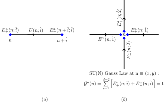
Figure 1: The location of the left and right electric fields $E_{+}(n;\hat{i})$ and $E_{-}(n+\hat{i};\hat{i})$ of a flux operator $U(n;i)$: (a) on a link $(n;i)$, (b) around a lattice site $n=(x,y)$. The SU(N) Gauss law is also pictorially shown in (b).

The kinematical variables involved in Kogut and Susskind Hamiltonian formulation kogut of lattice gauge theories are $SU(N)$ link operators $U(n;\hat{i})$ and the corresponding conjugate link electric fields $E^{a}_{+}(n;\hat{i})$ and $E^{a}_{-}(n+\hat{i};\hat{i})$. These electric fields rotate $U(n;\hat{i})$ from left and right as shown in Figure 1-a and satisfy the following canonical commutation relations

$$\left[E^{a}_{+}(n;\hat{i}),U_{\alpha\beta}(n;\hat{i})\right] = -\left(\frac{\lambda^{a}}{2}~{}U(n;\hat{i})\right)_{\alpha\beta}$$ (1)

$$\left[E^{a}_{-}(n+\hat{i};\hat{i}),U_{\alpha\beta}(n;\hat{i})\right] = ~{}~{}\left(U(n;\hat{i})~{}\frac{\lambda^{a}}{2}\right)_{\alpha\beta}$$

In (1), $\lambda^{a}~{}(a=1,2,\cdots,(N^{2}-1))$ are the representation matrices in the SU(N) fundamental representation satisfying $Tr\left(\lambda^{a}\lambda^{b}\right)=({1}/{2})\delta^{ab}$. The above SU(N) transformations imply that

$$\left[E^{a}_{+}(n;\hat{i}),E^{b}_{+}(n;\hat{i})\right] = if^{abc}E^{c}_{+}(n;\hat{i}),$$

$$\left[E^{a}_{-}(n;\hat{i}),E^{b}_{-}(n;\hat{i})\right] = if^{abc}E^{c}_{-}(n;\hat{i})$$ (2)

Above $f^{abc}$ are the SU(N) structure constants. We also define the strong coupling vacuum state $|0\rangle$ by demanding $E_{\mp}^{a}(n;\hat{i})|0\rangle=0$ on every link. The link operators $U(n;\hat{i})$ satisfy the following SU(N) conditions:

$$U(n;\hat{i})~{}U^{\dagger}(n;\hat{i})={\cal I},~{}~{}U^{\dagger}(n;\hat{i})~{}U(n;\hat{i})={\cal I}.$$ (3)

Above ${\cal I}$ is an $N\times N$ identity operator. Further, the determinant of the unitary matrix is also unity on every link: $|U(n;\hat{i})|={\cal I}$. Acting on strong coupling vacuum, the flux operator $U(n;\hat{i})$ creates and annihilates SU(N) fluxes on the link $(n;\hat{i})$. The quantization relations (1) show that electric field operators $E^{a}_{+}(n;\hat{i})$ and $E^{a}_{-}(n;\hat{i})$ are the generators of the left and right gauge transformations on $U(n;\hat{i})$ and $U(n-\hat{i};\hat{i})$ respectively. This is also illustrated in Figure 1-b. The left and right electric fields of link operator $U(n;\hat{i})$ in (1) are related by

$$E_{-}^{a}(n+\hat{i};\hat{i})=-R_{ab}(U^{\dagger}(n;\hat{i}))~{}E_{+}^{b}(n;\hat{i}).$$ (4)

In (4) $R_{ab}(U)\equiv({1}/{2})Tr\left(\lambda^{a}U\lambda^{b}U^{\dagger}\right)$ is the rotation matrix satisfying $\tilde{R}(U)R(U)=R(U)\tilde{R}(U)={\cal I}$ where $\tilde{R}$ is the transpose of R. The relations (4) show that $E^{a}_{-}(n;\hat{i})$ and $E^{b}_{+}(m,j)$ mutually commute: $[E^{a}_{-}(n;\hat{i}),E^{b}_{+}(m;\hat{j})]=0$ and their magnitudes are equal

$$\sum_{a=1}^{N^{2}-1}{E}^{a}_{+}(n;\hat{i}){E}^{a}_{+}(n;\hat{i}) = \sum_{a=1}^{N^{2}-1}E^{a}_{-}(n+\hat{i};\hat{i})E^{a}_{-}(n+\hat{i};\hat{i})$$ (5)

$$\equiv E^{2}(n;\hat{i}),~{}~{}~{}~{}~{}\forall~{}(n;\hat{i})$$

The SU(N) gauge transformations are:

$$E_{\pm}(n;\hat{i}) \rightarrow \Lambda(n)~{}E_{\pm}(n;\hat{i})~{}\Lambda^{\dagger}(n),$$ (6)

$$U(n;\hat{i}) \rightarrow \Lambda(n)~{}U(n;\hat{i})~{}\Lambda^{\dagger}(n+\hat{i}).$$

In (6) we have defined $E_{\pm}\equiv\sum_{a}E_{\pm}^{a}~{}\frac{\lambda^{a}}{2}$. The commutation relations (1) along with the gauge transformations (6) imply that the generators of SU(N) gauge transformations at a lattice site n are:

$${\cal G}^{a}(n)=\sum_{i=1}^{d}\Big{(}E_{-}^{a}(n;\hat{i})+E_{+}^{a}(n;\hat{i})\Big{)},~{}~{}\forall~{}~{}n,~{}a.$$ (7)

The SU(N) Gauss law (7) is illustrated in Figure 1-b. The Gauss law constraints, ${\cal G}^{a}(n)\approxeq 0,$ are imposed on the states to get physical states in ${\cal H}^{p}$. As discussed in the introduction, the obvious and the simplest gauge invariant basis in ${\cal H}^{p}$ is obtained by acting all possible Wilson loop operators $Tr{W}_{\gamma}$ on the strong coupling vacuum. Here, ${W}_{\gamma}$ is the holonomy operator corresponding to a closed, oriented loop $\gamma$. However, not all Wilson loop operators are mutually independent and therefore the above basis is over-complete. This over-completeness can be appreciated by considering the simplest SU(2) example loll ; manuplb :

$$Tr\left({W}_{\gamma}{W}_{\bar{\gamma}}\right)|0\rangle\equiv Tr{W}_{\gamma}Tr{W}_{\bar{\gamma}}|0\rangle-Tr\left({W}_{\gamma}{W}_{\bar{\gamma}}^{-1}\right)|0\rangle$$ (8)

involving any two arbitrary closed oriented loops denoted by $\gamma,\bar{\gamma}$ with a common starting and end point which can be anywhere on the lattice. This trivial example shows that the three Wilson loop states in (8) are not mutually independent. In the entire loop Hilbert space, involving all possible loops, there are numerous such relations even on a small lattice loll ; manuplb . Therefore, the gauge theory rewritten in the Wilson loop basis contains many redundant and spurious loop degrees of freedom manuplb . These mutual dependence of loop states are expressed by Mandelstam constraints like (8) in the case of SU(2) lattice gauge theory. These Mandelstam constraints are difficult to solve in terms of independent loop coordinates loll because of their large number and their non-local nature. As mentioned earlier, the problem of over-completeness of Wilson loop states becomes more and more difficult as we go to higher dimension and larger SU(N) groups migdal ; bishop ; manuplb ; rmi2 .

In the next section, using canonical transformations, we construct a complete set of fundamental SU(N) loop operators which are mutually independent. Thus the problems associated with SU(N) Mandelstam constraints, namely too many loop degrees of freedom, are completely bypassed for any N. At the same time, unlike the dual approaches mentioned above, the important SU(2) magnetic field terms reduce to a sum of gauge invariant SU(1,1) creation-annihilation operators (see eqn. (46) and (81)). These SU(1,1) operators $(k_{0},k_{+},k_{-})$ count, create and destroy the fundamental plaquette loops respectively as discussed in the next sections.

Figure 2: The plaquette loop operator ${\cal W}(x,y)$ & the string flux operator ${\sf T}(x,y)$ and their electric fields ${\cal E}^{a}_{\mp}(x,y)$ & ${\sf E}^{a}_{\mp}(x,y)$ respectively. Note that the electric fields ${\cal E}^{a}_{\mp}(x,y),~{}{\sf E}^{a}_{\mp}(x,y)$ are located at the initial and final points of the loops & strings respectively.

III SU(N) Canonical Transformations:  From links to loops & strings

We start with a set of ${\cal L}$ standard SU(N) Kogut-Susskind flux and their left, right conjugate electric field operators: $\Big{(}E^{a}_{+}(n;\hat{i}),U(n;\hat{i}),E_{-}^{a}(n+\hat{i};\hat{i})\Big{)}$ satisfying (1) and shown in Figure 1-a. We construct an iterative series of canonical transformations to transform them into:

• a set of ${\cal P}$ “physical” SU(N) plaquette loop flux operators and their conjugate loop electric fields:

  $$\Big{(}{\cal E}^{a}_{-}(n),~{}{\cal W}(n),~{}{\cal E}^{a}_{+}(n)\Big{)},~{}~{}~{}a=1,2,\cdots,N^{2}-1,$$

• a set of independent $({\cal N}-1)$ “unphysical” SU(N) string flux operators and their conjugate string electric fields:

  $$\Big{(}{\sf E}^{a}_{-}(n),~{}{\sf T}(n),~{}{\sf E}^{a}_{+}(n)\Big{)},~{}~{}~{}a=1,2,\cdots,N^{2}-1.$$

These new loop & string flux operators and the location of their electric fields are shown in Figure 2. As is clear from this figure, the convention chosen for loop & string electric fields is that ${\cal E}_{-}^{a}(n),{\sf E}_{-}^{a}(n)~{}\left({\cal E}_{+}^{a}(n),{\sf E}_{+}^{a}(n)\right)$ are located at the initial (final) points of the loop & string flux lines. They satisfy canonical commutation relations amongst themselves. The degrees of freedom exactly match as ${\cal L}={\cal P}+({\cal N}-1)$. We will show that the right electric field operators of the string attached to a site $n$ are the Gauss law generators (7) at n:

$${\sf E}^{a}_{+}(n)={\cal G}^{a}(n).$$ (9)

Therefore, all $({\cal N}-1)$ string flux operators ${\sf T}(n)$ create unphysical states $\notin{\cal H}^{p}$ and hence can be ignored without any loss of physics. The traces of ${\cal P}$ plaquette loop flux operators of the form

$$Tr\Big{(}({\cal W}(n_{1}))^{q_{1}}({\cal W}(n_{2}))^{q_{2}}\cdots({\cal W}(n_{p}))^{q_{\cal P}}\Big{)}$$

create-annihilate all possible physical loop states in ${\cal H}^{p}$. Above $(q_{1},q_{2},\cdots,q_{{}_{\cal P}})$ are sets of ${\cal P}$ integers. We now discuss the canonical transformations. To keep the discussion simple, we start with a single plaquette case before dealing with the entire lattices in $d=2,3$. Some of the issues in this section were covered briefly in ms1 .

III.1 Canonical transformations on a single plaquette

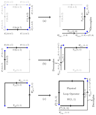
Figure 3: Three canonical transformations on the four link flux operators of a plaquette OABC leading to a single physical plaquette loop flux operator ${\cal W}_{\alpha\beta}(1,1)$ in (c). The three right electric fields $\sf E^{a}_{[xy]+}(1,0),~{}\sf E^{a}_{[xy]+}(1,1),~{}\sf E^{a}_{[xy]+}(0,1)$ of the three string flux operators ending at A, B and C respectively are the Gauss law generators ${\cal G}^{a}(A),~{}{\cal G}^{a}(B)$ and ${\cal G}^{a}(C)$ respectively. The Gauss law at the origin is: ${\cal G}^{a}(O)=E^{a}_{+}(0,0;\hat{1})+E^{a}_{+}(0,0;\hat{2})={\cal E}_{-}^{a}(1,1)+{\cal E}_{+}^{a}(1,1)=0$.

We start with a plaquette OABC with the following Kogut-Susskind SU(N) link flux operators kogut : $\left(E^{a}_{+}(0,0;\hat{1}),~{}U(0,0;\hat{1}),~{}E_{-}^{a}(1,0;\hat{1})\right)$ on link OA,  $\left(E^{a}_{+}(1,0;\hat{2}),U(1,0;\hat{2}),E^{a}_{-}(1,1;\hat{2})\right)$ on link AB,  $\left(E^{a}_{+}(0,1;\hat{1}),~{}U(0,1;\hat{1}),~{}E^{a}_{-}(1,1;\hat{1})\right)$ on link CB and finally the operators $(E^{a}_{+}(0,0;\hat{2}),~{}U(0,0;\hat{2}),~{}E^{a}_{-}(0,1;\hat{2}))$ on the link OC. These link operators and their locations are clearly illustrated on the left hand side of Figure 3-a. As is clear from this figure, the SU(N) Gauss laws at four corners O, A, B and C are:

$${\cal G}^{a}(0,0) = E^{a}_{+}(0,0;\hat{1})+E^{a}_{+}(0,0;\hat{2})=0;$$

$${\cal G}^{a}(1,0) = E^{a}_{-}(1,0;\hat{1})+E^{a}_{+}(1,0;\hat{2})=0;$$

$${\cal G}^{a}(1,1) = E^{a}_{-}(1,1;\hat{2})+E^{a}_{-}(1,1;\hat{1})=0;$$

$${\cal G}^{a}(0,1) = E^{a}_{+}(0,1;\hat{1})+E^{a}_{-}(0,1;\hat{2})=0.$$ (10)

We now make canonical transformations to fuse ${\cal L}$ (=4) Kogut Susskind SU(N) flux operators $U(0,0;\hat{1}),~{}U(1,0;\hat{2}),~{}U(0,1;\hat{1})$ and $U(0,0;\hat{2})$ into ${\cal N}-1$ (= 3) unphysical string flux operators $\Big{[}{\sf T}_{[xy]}(1,0),{\sf T}_{[xy]}(1,1),{\sf T}_{[xy]}(0,1)\Big{]}$ and ${\cal P}~{}(=1)$ physical SU(N) plaquette loop flux operator ${\cal W}(1,1)$ around the plaquette OABC as shown in Figure 3. The corresponding right string and loop electric fields are denoted by $\Big{[}{\sf E}_{[xy]+}^{a}(1,0),{\sf E}_{[xy]+}^{a}(1,1),{\sf E}_{[xy]+}^{a}(1,0)\Big{]}$ and ${\cal E}_{+}^{a}(1,1)$ respectively. All left electric field operators are defined using (4).

The canonical transformations are performed in 3 sequential steps as shown in Figure (3-a), (3-b) and (3-c) respectively. The first canonical transformation fuses $U(0,0;\hat{1})$ with $U(1,0;\hat{2})$ into ${\sf T}_{[xy]}(1,0)$ and ${{\sf T}}_{[y]}(1,1)$ as follows:

$${\sf T}_{[xy]}(1,0)\equiv U(0,0;\hat{1}),~{}~{}{{\sf T}}_{[y]}(1,1)\equiv U(0,0;\hat{1})U(1,0;\hat{2}),$$ (11)

$$~{}~{}{{\sf E}}_{[xy]+}^{a}(1,0)=E^{a}_{-}(1,0;\hat{1})+{E}^{a}_{+}(1,0;\hat{2})\equiv{\cal G}^{a}(1,0),$$

$${{\sf E}}^{a}_{[y]+}(1,1)={E}^{a}_{-}(1,1;\hat{2}).$$

All steps in (11) are also illustrated in Figure 3-a. Note that the resulting new canonical pairs $\left({\sf T}_{[xy]}(1,0),{\sf E}_{[xy]+}(1,0)\right)$ and $\left({\sf T}_{[y]}(1,1),{\sf E^{a}}_{[y]+}(1,1)\right)$ satisfy the standard canonical commutation relations simply by construction in (11):

$$\left[\sf E^{a}_{[xy]+}(1,0),{\sf T}_{[xy]}(1,0)\right]=\sf T_{[xy]}(1,0)\left(\frac{\lambda^{a}}{2}\right),$$

$$\left[{\sf E}_{[y]+}^{a}(1,1),T_{[y]}(1,1)\right]={\sf T}_{[y]}(1,1)\left(\frac{\lambda^{a}}{2}\right).$$ (12)

They are also mutually independent:

$$\left[\sf E^{a}_{[xy]+}(1,0),{\sf T}_{[y]}(1,1)\right]=0,~{}~{}\left[{\sf E}^{a}_{[y]}(1,1),{\sf T}_{[xy]}(1,0)\right]=0.$$

$$\left[\sf E^{a}_{[xy]+}(1,0),{\sf E}_{[y]}(1,1)\right]=0,~{}~{}\left[{\sf T}_{[y]}(1,1),{\sf T}_{[xy]}(1,0)\right]=0.$$

Therefore the resulting new canonical pairs should be treated exactly on the same footing as the initial Kogut-Susskind canonical pairs on links. The left electric fields are given by

$$\sf E^{a}_{[xy]-}(1,0) \equiv -R_{ab}\left({\sf T}_{[xy]}(1,0)\right){\sf E}^{b}_{[xy]+}(1,0),$$

$$\sf E^{a}_{[y]-}(1,1) \equiv -~{}R_{ab}(\sf T_{[y]}(1,1))~{}~{}\sf E^{b}_{[y]+}(1,1).$$ (13)

From the third equation in (11) and ${\cal G}^{a}(1,0)=0$, it is clear that the string flux operator $\sf T_{[xy]}(1,0)$ is unphysical as its action on any state takes that state out of ${\cal H}^{p}$. Therefore, we ignore it henceforth. We now iterate the above canonical transformations with $U(0,0;\hat{1}),~{}U(1,0;\hat{2})$ in (11) replaced by ${U}(0,0;\hat{2}),~{}U(0,1;\hat{1})$ respectively. We define:

$${\sf T}_{[xy]}(0,1)\equiv U(0,1;\hat{2}),~{}~{}{\sf T}_{[x]}(1,1)\equiv U(0,0;\hat{2})~{}U(0,1;\hat{1}),$$

$${\sf E}^{a}_{[xy]+}(0,1)={E}^{a}_{-}(0,1;\hat{2})+{E}^{a}_{+}(0,1;\hat{1})={\cal G}^{a}(0,1),$$

$${\sf E}^{a}_{[x]+}(1,1)=E^{a}_{-}(1,1;\hat{1}).$$ (14)

Again, the canonical transformations (14) are illustrated in Figure 3-b. The resulting two new canonical pairs of string operators $\left(\sf T_{[xy]}(0,1),\sf E^{a}_{[xy]+}(0,1)\right)$ and $\left(\sf T_{[x]}(1,1),\sf E^{a}_{[x]+}(1,1)\right)$ are canonical as well as mutually independent like the previous two sets in (12). The left electric fields ${\sf E}^{a}_{[xy]-}(0,1),~{}{\sf E}^{a}_{[x]-}(1,1)$ are again defined through parallel transports as in (4) or (13). As a consequence of Gauss law at C the string operator ${\sf T}_{[xy]}(0,1)$ (like $\sf T_{[xy]}(1,0)$) becomes unphysical. The last sets of canonical transformations fuse the remaining two strings ${\sf T}_{[y]}(1,1)$ and ${\sf T}_{[x]}(1,1)$ to define the final physical plaquette loop conjugate operators $\left({\cal W}(1,1),{\cal E}_{+}(1,1)\right)$:

$${\sf T}_{[xy]}(1,1)\equiv\sf T_{[y]}(1,1),~{}{\cal W}(1,1)\equiv\sf T_{[y]}(1,1)~{}{\sf T}^{\dagger}_{[x]}(1,1),$$

$${\sf E}_{[xy]+}(1,1)={\sf E}^{a}_{[y]+}(1,1)+{\sf E}^{a}_{[x]+}(1,1)={\cal G}^{a}(1,1)=0,$$

$${\cal E}^{a}_{+}(1,1)={\sf E}^{a}_{[x]-}(1,1).~{}~{}~{}~{}~{}~{}~{}~{}~{}~{}~{}~{}~{}~{}~{}$$ (15)

The above canonical transformations are illustrated in Figure 3-c. In the third equation in (15), the right electric fields ${\sf E}^{a}_{[y]+}(1,1)$ and ${\sf E}^{a}_{[x]+}(1,1)$ have been substituted in terms of the Kogut-Susskind electric fields using (11) and (14) to get the SU(N) Gauss laws: ${\cal G}^{a}(1,1)=0$ at lattice site B. Now ${\sf T}_{[xy]}(1,1)$ decouples and

$${\cal W}(1,1)\equiv U(0,0;\hat{1})~{}U(1,0;\hat{2})U^{\dagger}(0,1;\hat{1})U^{\dagger}(0,0;\hat{2})$$ (16)

emerges as the final physical plaquette loop flux operator. Its left and right electric fields are :

$${\cal E}^{a}_{-}(1,1)=E^{a}_{+}(0,0;\hat{1}),~{}~{}{\cal E}^{a}_{+}(1,1)=E^{a}_{+}(0,0;\hat{2}).$$ (17)

Thus we have converted all link operators into string & loop operators. Note that by construction the canonical structures are rigidly maintained at all three steps ((11), (14) and (15)). The string flux operators and their conjugate electric fields satisfy

$$\left[{\sf E}^{a}_{[xy]+}(x,y),{\sf T}(x^{\prime},y^{\prime})\right] = \delta_{x,x^{\prime}}\delta_{y,y^{\prime}}\left({\sf T(x,y)}\frac{\lambda^{a}}{2}\right),$$

$$\left[{\sf E}^{a}_{+}(x,y),{\sf E}^{b}_{+}(x^{\prime},y^{\prime})\right] = i\delta_{x,x^{\prime}}\delta_{y,y^{\prime}}f^{abc}{\sf E}^{c}_{+}(x,y).~{}~{}~{}~{}~{}$$ (18)

Above $(x,y),~{}(x^{\prime},y^{\prime})=(1,0),(1,1),(0,1)$. The string electric fields ${\sf E}_{[xy]+}^{a}(x,y)$ at $(x,y)$ satisfy SU(N) algebra and commute if they are at different lattice sites. Under SU(N) gauge transformations, these string operators transform as:

$${\sf T}_{[xy]}(x,y) \rightarrow \Lambda(0,0)~{}{\sf T}_{[xy]}(x,y)\Lambda^{\dagger}(x,y),$$

$${\sf E}_{[xy]+}(x,y) \rightarrow \Lambda(x,y){\sf E}_{[xy]+}(x,y)\Lambda^{\dagger}(x,y).$$ (19)

Therefore, none of the three strings can form any gauge invariant operators at their end points $(0,1),(1,1),(0,1)$. The SU(N) Gauss laws at A, B, C state this simple fact. Having removed the three unphysical strings, we now focus on the plaquette loop operators $\left({\cal E}_{-}^{a}(1,1),~{}{\cal W}(1,1),~{}{\cal E}_{+}^{a}(1,1)\right)\equiv\left({\cal E}_{-}^{a},~{}{\cal W},~{}{\cal E}_{+}^{a}\right)$. Again by construction, they satisfy the canonical quantization relations:

$$\left[{\cal E}^{a}_{+},{\cal W}\right] = -\left(\frac{\lambda^{a}}{2}{\cal W}\right)\Rightarrow\left[{\cal E}^{a}_{+},{\cal E}^{b}_{+}\right]=if^{abc}{\cal E}^{c}_{+},~{}~{}~{}~{}~{}~{}$$

$$\left[{\cal E}^{a}_{-},{\cal W}\right] = ~{}~{}\left({\cal W}\frac{\lambda^{a}}{2}\right)~{}\Rightarrow\left[{\cal E}^{a}_{-},{\cal E}^{b}_{-}\right]=if^{abc}{\cal E}^{c}_{-}.$$ (20)

Above ${\cal E}^{a}_{-}\equiv-R_{ab}({\cal W})~{}{\cal E}^{b}_{+}$ implying $(\vec{\cal E}_{-})^{2}=(\vec{\cal E}_{+})^{2}\equiv(\vec{\cal E})^{2}$ and $[{\cal E}^{a}_{-},{\cal E}^{b}_{+}]=0$. They gauge transform at the origin as:

$${\cal E}_{\mp}\rightarrow\Lambda~{}{\cal E}_{\mp}~{}\Lambda^{\dagger},~{}~{}~{}~{}~{}~{}{\cal W}\rightarrow\Lambda~{}{\cal W}~{}\Lambda^{\dagger}.$$ (21)

We have defined ${\cal E}_{\mp}\equiv\sum_{a}{\cal E}_{\mp}^{a}~{}\lambda^{a}$ and $\Lambda\equiv\Lambda(0,0)$ denotes the gauge rotation at the origin. The corresponding Gauss law at the origin is:

$${\cal G}^{a}(0,0)={\cal E}_{-}^{a}+{\cal E}_{+}^{a}=E^{a}_{+}(0,0;\hat{1})+E^{a}_{+}(0,0;\hat{2})=0.~{}~{}~{}$$ (22)

The relations (22) are valid within ${\cal H}^{p}$ because we have ignored all string electric fields because of the Gauss laws: ${\sf E}_{[xy]}^{a}(x,y)=0,~{}(x,y)=(1,0),(1,1),(0,1)$.

III.1.1 Inverse relations

It is instructive and useful to invert the canonical transformations (11), (14) and (15) to write Kogut Susskind link operators in terms of strings and loop variables. These relations also enable us to write the Kogut Susskind Hamiltonian (42) in terms of loop operators (see (43)). It is clear from Figure 3-a,b,c that

$$U(0,0;\hat{1})=\sf T(1,0),~{}~{}U(1,0;\hat{2})=\sf T^{\dagger}(1,0)\sf T(1,1)~{}$$ (23)

$$U(0,0;\hat{2})=\sf T(0,1),~{}~{}U(0,1;\hat{1})=\sf T^{\dagger}(0,1){\cal W}^{\dagger}\sf T(1,1).$$

Above we have ignored subscript $[xy]$ and used ${\sf T}(x,y)\equiv{\sf T}_{[xy]}(x,y)$. Similarly, the electric field relations in (11), (14) and (15) can also be inverted to write (see appendix B for details):

$$E_{+}^{a}(0,0;\hat{1}) = {\sf E}^{a}_{[xy]-}(1,0)+{\sf E}^{a}_{[xy]-}(1,1)+{\cal E}^{a}_{-},$$

$$E_{+}^{a}(1,0;\hat{2}) = R_{ab}\left({\sf T}^{\dagger}_{[xy]}(1,0)\right)\Big{(}{\sf E}^{b}_{[xy]-}(1,1)+{\cal E}^{b}_{-}\Big{)},$$

$$E_{+}^{a}(0,0;\hat{2}) = {\cal E}_{+}^{a}+{\sf E}^{a}_{[xy]-}(0,1),$$

$$E_{+}^{a}(0,1;\hat{1}) = R_{ab}\left({\sf T}^{\dagger}_{[xy]}(0,1)\right)~{}{\cal E}_{+}^{b}.$$ (24)

These canonical relations between links & loops have the following interesting features:

• They are consistent with gauge transformations (6), (19) and (21) as well as with SU(N) algebras of link, string and loop electric fields given in (1) and (18), (20).

• The canonical commutation relations between SU(N) link flux operators and their link electric fields also remain intact under the links to loops & stings mappings (23) and (III.1.1).

• No strings (${\sf T}(x,y)$ or ${\sf E}^{a}(x,y)$) can appear in a gauge invariant operator in ${\cal H}^{p}$. As an example, the gauge invariant electric field terms in the Kogut Susskind Hamiltonian are:

  $$\left(\vec{E}_{+}(0,0;\hat{1})\right)^{2}=\left(\vec{E}_{+}(1,0;\hat{2})\right)^{2}=\left(\vec{E}_{+}(0,1;\hat{1})\right)^{2}$$

  $$=\left(\vec{E}_{+}(0,0;\hat{2})\right)^{2}=\left(\vec{\cal E}_{-}\right)^{2}.$$ (25)

  We have used the Gauss laws ${\sf E}^{a}_{[xy]+}(x,y)=0$ in (III.1.1) within ${\cal H}^{p}$. In other words, while expressing Kogut-Susskind link electric fields in terms of loop electric fields, the strings can appear only in the overall parallel transport factors. This is also required for the consistency with SU(N) gauge transformations in (III.1.1).

III.1.2 Loop prepotential operators

The physical loop electric fields ${\cal E}_{\pm}^{a}$ discussed in the previous section can be conveniently described in terms of the prepotential creation-annihilation operators:

$${\cal E}_{-}^{a}=a^{\dagger}~{}\left(\frac{\sigma^{a}}{2}\right)~{}a,~{}~{}~{}~{}~{}~{}~{}~{}~{}~{}{\cal E}_{+}^{a}=b^{\dagger}~{}\left(\frac{\sigma^{a}}{2}\right)~{}b.$$ (26)

In (26) ${\cal E}_{\pm}^{a}$ are SU(2) electric fields and $(a^{\dagger}_{\alpha},b^{\dagger}_{\beta})$ and $\left(a_{\alpha},b_{\beta}\right)$ are the SU(2) prepotential creation and annihilation SU(2) doublets with $\alpha,\beta=1,2$. We also define the total number operators $\hat{N}_{a}=a^{\dagger}\cdot a\equiv a^{\dagger}_{1}a_{1}+a^{\dagger}_{2}a_{2}$,  $\hat{N}_{b}=b^{\dagger}\cdot b\equiv b^{\dagger}_{1}b_{1}+b^{\dagger}_{2}b_{2}$. The constraint ${\cal E}_{+}^{2}={\cal E}_{-}^{2}$ implies

$$\hat{N}_{a}=\hat{N}_{b}\equiv\hat{N}.$$

Under SU(2) gauge transformations (21):

$$a_{\alpha}\rightarrow\Lambda_{\alpha\beta}~{}a_{\beta},~{}~{}~{}~{}b_{\alpha}\rightarrow\Lambda_{\alpha\beta}~{}b_{\beta}.$$ (27)

The prepotential formulation also has an important additional U(1) invariance manujp ; manuplb :

$$a_{\alpha}\rightarrow e^{i\theta}~{}a_{\alpha},~{}~{}~{}b_{\alpha}\rightarrow e^{-i\theta}~{}b_{\alpha}.$$ (28)

The prepotential operators defining relations (26) are invariant under (28). The gauge invariant strong coupling vacuum $|0\rangle~{}(\equiv|0\rangle_{a}\otimes|0\rangle_{b})$ is also the prepotential harmonic oscillator vacuum satisfying: $a_{\alpha}|0\rangle=0,~{}~{}b_{\alpha}|0\rangle=0.$ The quantization rules (1) and the gauge transformations (21), (28) imply manujp ; manuplb :

$${\cal W}_{\alpha\beta} = \frac{1}{\sqrt{(\hat{N}+1)}}\left(a_{\alpha}\tilde{b}_{\beta}-\tilde{a}^{\dagger}_{\alpha}b^{\dagger}_{\beta}\right)\frac{1}{\sqrt{(\hat{N}+1)}}~{}~{}~{}~{}~{}~{}~{}~{}$$ (29)

$$\equiv \frac{1}{\sqrt{(\hat{N}+1)}}\left({\cal W}^{(-)}_{\alpha\beta}+{\cal W}^{(+)}_{\alpha\beta}\right)\frac{1}{\sqrt{(\hat{N}+1)}}.$$

It is easy to check that (26) and (29) satisfy the canonical commutation relations (20). Further, the above prepotential representation also maintains the non-trivial relations: ${\cal W}~{}{\cal W}^{\dagger}={\cal W}^{\dagger}~{}{\cal W}={\cal I},~{}|{\cal W}|=+1$ as well as the canonical commutation relations: $\left[{\cal W}_{\alpha\beta},{\cal W}_{\gamma\delta}\right]=0,~{}~{}\left[{\cal W}_{\alpha\beta},{\cal W}^{\dagger}_{\gamma\delta}\right]=0.$

We now construct a complete orthonormal loop basis in ${\cal H}^{p}$ with the prepotential operators in a straightforward manner in the next section. We further show that ${\cal H}^{p}$ can be exactly identified with all possible spherically symmetric “s-states of a hydrogen atom” ms1 .

III.1.3 Physical loop Hilbert space and Hydrogen atom

In the standard approach all four link flux operators in Figure 3-a are fundamental with each of them gauge transforming differently. Therefore, the construction of gauge invariant states is more involved compared to working with a single loop flux operator ${\cal W}$. In this section we exploit this simple fact and show that the physical or loop Hilbert space can be completely realized in terms of a hydrogen atom Hilbert space. This correspondence is achieved by identifying the loop electric fields $\vec{\cal E}_{\mp}$ of SU(2) lattice gauge theory with the angular momentum $\vec{\sf L}$ and Laplace Runge Lenz vector $\vec{\sf A}$ of the hydrogen atom. More precisely:

$$\vec{\cal E}_{\mp}\equiv\frac{1}{2}\left(\vec{\sf L}\mp\vec{\sf A}\right).$$ (30)

In the above identification, the identity $\vec{\cal E}_{-}^{~{}2}=\vec{\cal E}_{+}^{~{}2}\equiv\vec{\cal E}^{~{}2}$ in (5) holds naturally as $\vec{\sf L}\cdot\vec{\sf A}=0$ wyb . We can also have three separate identifications like (30) for the three string electric fields ${\sf T}_{[xy]\mp}(1,0),~{}{\sf T}_{[xy]\mp}(1,1),~{}{\sf T}_{[xy]\mp}(0,1)$. But these identifications will be in the unphysical sector in the case of pure gauge theories and hence we ignore them in this work.

We first construct the eigenstates of the complete set of commuting operators (CSCO-I) consisting of $(\vec{\cal E}_{-}^{~{}2}\equiv\vec{\cal E}^{~{}2},~{}{\cal E}_{-}^{a=3})$ and $(\vec{\cal E}_{+}^{~{}2}\equiv\vec{\cal E}^{~{}2},~{}{\cal E}_{+}^{a=3})$ which form $SU(2)\otimes SU(2)$ representations:

$$|j,m_{-},m_{+}\rangle=\underbrace{T^{j}_{m_{-}}(a^{\dagger})~{}|0\rangle_{a}}_{|j,m_{-}\rangle_{a}}~{}\otimes~{}\underbrace{T^{j}_{m_{+}}(b^{\dagger})~{}|0\rangle_{b}}_{|j,m_{+}\rangle_{b}}.$$ (31)

In (31), the tensor operator $T^{j}_{m}$ are defined as

$$T^{j}_{m}(a^{\dagger})\equiv\sqrt{(2j)!}\left(\frac{(a^{\dagger}_{1})^{(j+m)}(a^{\dagger}_{2})^{(j-m)}}{\sqrt{(j+m)!(j-m)!}}\right).$$

The states (31) are invariant under U(1) gauge transformations (27). They are eigenstates of the above CSCO-I:

$$\vec{\cal E}^{~{}2}|j,m_{-},m_{+}\rangle=j(j+1)|j,m_{-},m_{+}\rangle,$$

$$\vec{\cal E}_{\mp}^{a=3}|j,m_{-},m_{+}\rangle=m_{\mp}|j,m_{-},m_{+}\rangle.$$ (32)

In the context of hydrogen atom, the states (31) are the energy eigen states with energy wyb $E_{\sf n}\sim\frac{1}{{\sf n}^{2}}$ with ${\sf n}\equiv 2j+1$. The two magnetic quantum numbers $m_{\mp}$ describe their degeneracies. On the other hand, in the gauge theory context the states $|j~{}m_{-}~{}m_{+}\rangle$ in (32) describe loops carrying non-abelian quantized SU(2) loop electric fluxes . Further, as ${\cal E}_{-}^{a}+{\cal E}_{+}^{a}\equiv{\sf L}^{a}$ the gauge rotations at the origin of the flux states in (31) correspond to the spatial rotations of the hydrogen atom. Under these gauge transformations:

$$|jm_{-}{m}_{+}\rangle\rightarrow\sum_{m_{\mp}^{\prime}}|jm^{\prime}_{-}{m}^{\prime}_{+}\rangle D^{~{}~{}j}_{m^{\prime}_{-}m_{-}}(\Lambda)~{}D^{~{}~{}j}_{{m}^{\prime}_{+}{m}_{+}}(\Lambda).$$ (33)

In (33), $D^{~{}~{}j}_{mm^{\prime}}(\Lambda)$ are the Wigner matrices, $\Lambda\equiv\Lambda(0,0)$ denotes the gauge parameters at the origin. We have used the gauge transformations (27) and the definition (31) to get (33). In order to solve Gauss law systematically, we construct a coupled basis from (31) so that the following coupled and complete set of commuting operators (CSCO II) are diagonal:

$$\left\{\vec{\cal E}_{-}^{~{}2}=\vec{\cal E}_{+}^{~{}2}=\vec{\cal E}^{~{}2},~{}~{}~{}(\vec{\cal E}_{-}+\vec{\cal E}_{+})^{2},~{}~{}~{}(\vec{\cal E}_{-}+\vec{\cal E}_{+})^{a=3}\right\}$$

$$\equiv\left\{\vec{\cal E}^{2},~{}(\vec{\sf L})^{2},~{}(\vec{\sf L})^{a=3}\right\}.$$

The eigenbasis states of CSCO-I and CSCO-II are related by Clebsch-Gordan coefficients:

$$|{\sf n}~{}l~{}m\rangle\equiv\sum_{m_{-},m_{+}}C_{jm_{-},jm_{+}}^{~{}~{}l,m}~{}|j~{}m_{-}m_{+}\rangle$$

$$=\sum_{m_{-},m_{+}}C_{jm_{-},jm_{+}}^{~{}~{}l,m}~{}|j,m_{-}\rangle_{a}~{}|j,m_{+}\rangle_{b}.$$ (34)

Above ${\sf n}\equiv 2j+1=1,2,\cdots;~{}~{}~{}l=0,1,\cdots,2j~{}(\equiv{\sf n}-1);~{}~{}~{}m=-l,-(l-1),\cdots,(l-1),l$. The states in (34) are eigenstates of CSCO II:

$$\vec{\cal E}^{~{}2}~{}|{\sf n}~{}l~{}m\rangle ~{}=~{}\frac{({\sf n}^{2}-1)}{4}~{}~{}|{\sf n}~{}l~{}m\rangle,$$

$$\vec{\sf L}^{~{}2}~{}|{\sf n}~{}l~{}m\rangle ~{}=~{}l(l+1)~{}~{}|{\sf n}~{}l~{}m\rangle,$$

$${\sf L}^{a=3}~{}|{\sf n}~{}l~{}m\rangle ~{}=~{}~{}~{}m~{}~{}|{\sf n}~{}l~{}m\rangle.$$ (35)

Note that the states $|{\sf n}~{}l~{}m\rangle$ in (34) are also the standard hydrogen atom energy eigenstates wyb characterized by the principal, angular momentum and magnetic quantum numbers ${\tt n},~{}l$ and $m$ respectively. Under gauge transformations, the coupled states (34) have much simpler transformation property as compared to the states in (33):

$$|{\sf n}~{}l~{}m\rangle\rightarrow\sum_{\bar{m}}D^{~{}l}_{m\bar{m}}(\Lambda)~{}|{\sf n}~{}l~{}\bar{m}\rangle.$$ (36)

Thus the principal and angular momentum quantum numbers are gauge invariant. The Gauss law in this single plaquette case (22) states that ${\cal E}^{a}_{-}+{\cal E}^{a}_{+}\equiv{\sf L}^{a}=0$. Therefore, all possible orthonormal solutions are the s-states $|{\sf n},l=0,m=0\rangle$ of hydrogen atom. This gauge invariant hydrogen atom loop basis can be easily constructed in terms of the prepotential operators. There are three possible $SU(2)\times U(1)$ gauge invariant operators:

$$k_{-}\equiv a\cdot\tilde{b},~{}~{}k_{+}\equiv a^{\dagger}\cdot\tilde{b}^{\dagger},~{}~{}k_{0}\equiv\frac{1}{2}~{}\underbrace{(\hat{N}_{a}+\hat{N}_{b}+2)}_{2(\hat{N}+1)}$$ (37)

In (37) $a\cdot\tilde{b}=a_{\alpha}\tilde{b}_{\alpha}=a_{\alpha}\epsilon_{\alpha\beta}b_{\beta}\equiv(a_{1}b_{2}-a_{2}b_{1})$ and $\hat{N}_{a}=\hat{N}_{b}=\hat{N}$. They are gauge invariant loop creation-annihilation operators $k_{\pm}={\rm Tr}{\cal W}^{(\pm)}$. On the other hand, gauge invariant $k_{0}$ has the interpretation of loop flux counting operator. They satisfy SU(1,1) algebra:

$$\left[k_{-},k_{+}\right]=2k_{0},~{}~{}~{}~{}~{}~{}~{}~{}~{}\left[k_{0},k_{\pm}\right]=\pm k_{\pm}.$$ (38)

They are also invariant under U(1) transformations (28). The SU(1,1) Casimir operator is defined as:

$${\cal C}\equiv k_{0}^{2}-\frac{1}{2}\left(k_{-}k_{+}+k_{+}k_{-}\right).$$ (39)

All possible orthonormal hydrogen atom loop states can be easily constructed using SU(1,1) or loop creation operators $k_{+}$:

$$|{\sf n}\rangle~{}\equiv~{}\frac{1}{\sqrt{({\sf n}-1)!~{}{\sf n}!}}~{}\left(k_{+}\right)^{{\sf n}-1}|0\rangle;~{}~{}~{}{\sf n}=1,2\cdots.$$ (40)

The single plaquette loop states in (40) form a discrete representation of SU(1,1) with Bargmann index ${\mathtt{k}}=1$:

$${\cal C}\ket{\tt n}=0,~{}~{} ~{}~{}k_{0}\ket{\tt n}=\tt n\ket{\tt n}$$ (41)

$$k_{+}\ket{\tt n}=\sqrt{\tt n(\tt n+1)}~{}\ket{\tt n+{1}}, k_{-}\ket{\tt n}=\sqrt{\tt n(\tt n-1)}\ket{\tt n-{1}}$$

These gauge invariant fundamental loop flux creation-annihilation and counting operators govern the loop dynamics which we discuss in the next section. Note that in the hydrogen atom loop basis all topological effects of the compactness of SU(2) gauge group are contained in the discreteness of the principal quantum numbers ${\tt n}$ of hydrogen atom.

III.1.4 Loop dynamics and $SU(1,1)\subset SO(4,2)$

We consider SU(N) Kogut-Susskind Hamiltonian kogut :

$$H = {g^{2}}\sum_{l=1}^{4}\vec{E}^{2}(l)+\frac{K}{g^{2}}\left[2N-{\textrm{T}r}\left(U_{1}~{}U_{2}~{}U_{3}^{\dagger}~{}U_{4}^{\dagger}~{}+~{}h.c~{}\right)\right]$$ (42)

$$\equiv~{}~{}~{}~{}~{}H_{E}~{}~{}+~{}~{}H_{B}.$$

In (42), K is a constant and $U_{1}\equiv U(0,0;\hat{1}),U_{2}\equiv U(1,0;\hat{2}),U_{3}\equiv U(0,1;\hat{1}),U_{4}\equiv U(0,0;\hat{2})$. Using links to loop relations (16) and (25), the SU(N) loop Hamiltonian for the single plaquette is:

$$H=4g^{2}\vec{\cal E}^{2}+\frac{K}{g^{2}}\left[2N-{\textrm{T}r}\left({\cal W}+{\cal W}^{\dagger}\right)\right].$$ (43)

At this stage we specialize to SU(2) case . The Hamiltonian (42) can be completely rewritten in terms of loop creation, annihilation and counting operators forming SU(1,1) algebra. The electric field term is:

$$H_{E}=g^{2}\sum_{l=1}^{4}\vec{E}^{2}(l)=4g^{2}\vec{\cal E}^{2}=g^{2}\left(k_{0}^{2}-1\right).$$ (44)

The four link magnetic field term takes its simplest possible form:

$$H_{B} =\frac{1}{g^{2}}~{}~{}Tr(U_{1}~{}U_{2}~{}U_{3}^{\dagger}~{}U_{4}^{\dagger})=\frac{1}{g^{2}}~{}~{}Tr~{}{\cal W}$$

$$=\frac{1}{g^{2}}~{}~{}\frac{1}{\sqrt{k_{0}}}~{}\Big{(}k_{-}+k_{+}\Big{)}~{}\frac{1}{\sqrt{k}_{0}}.$$ (45)

The magnetic field term, important in the weak coupling continuum limit, simply creates and annihilates the fluxes on the plaquette loop:

$$H_{B}~{}\ket{\sf n}~{} =\frac{1}{g^{2}}~{}Tr\left(U_{1}~{}U_{2}~{}U_{3}^{\dagger}~{}U_{4}^{\dagger}\right)\ket{\sf n}~{}=\frac{1}{g^{2}}~{}Tr~{}{\cal W}~{}|\sf n\rangle$$

$$=\frac{1}{g^{2}}~{}\Big{[}{\sf n}+{1}\rangle+\ket{{\sf n}-1}\Big{]}.$$ (46)

Note that the magnetic field term which was product of four (link) flux operators reduces to a single (loop) flux operator. This is the simplest possible form of the important $(1/g^{2})$ magnetic field term. In the Appendix C we show that the loop Schrödinger equation easily reduces to Mathieu equation in the magnetic basis.

In the case of finite lattice, considered in the next sections, the states (35) of hydrogen atoms are associated with every plaquette. Like in single plaquette case, they describe the electric fluxes flowing around the corresponding plaquettes. The Gauss law is solved by Wigner coupling all the hydrogen atom states and demanding that the three components of the total angular momenta vanish. Further, the role of SU(1,1) in this section gets generalized to the dynamical symmetry group SO(4,2) of hydrogen atoms (see section III.2.4).

III.2 Canonical transformations on a finite lattice

On a finite $d=2$ lattice we canonically transform the $3{\cal L}$ Kogut-Susskind conjugate operators $\left[U(x,y;\hat{i}),~{}E^{a}_{\mp}(x,y;\hat{i})\right]$ satisfying (1) on every link into

1. $3({\cal N}-1)$ unphysical string conjugate operators $\left[{\sf T}(x,y),{\sf E}^{a}_{\mp}(x,y)\right]$ satisfying (18) at every site. These operators are shown in Figure 2-a. The string ${\sf T}(x,y)$ start at $(0,0)$ and end at $(x,y)$ following the path $(0,0)\rightarrow(x,0)\rightarrow(x,y)$.

2. $3{\cal P}$ physical loop conjugate operators $\Big{[}{\cal W}(x,y),~{}{\cal E}^{a}_{\mp}(x,y)\Big{]}$ satisfying (20) on every plaquette or equivalently at every dual site. These operators are shown in Figure 2-b. The plaquette loop flux operator ${\cal W}(x,y)$ is along the path: $(0,0)\rightarrow(x-1,0)\rightarrow(x-1,y-1)\rightarrow(x,y-1)\rightarrow(x,y)\rightarrow(x-1,y)\rightarrow(x-1,0)\rightarrow(0,0)$.

The above two sets are mutually independent. As mentioned earlier, the total degrees of freedom match because ${\cal L}={\cal P}+({\cal N}-1)$.

III.2.1 Canonical relations

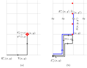
Figure 4: Graphical representation of the canonical relations (48). The Kogut Susskind electric fields are denoted by $\blacklozenge$ and the plaquette loop electric fields are denoted by $\bullet$. We show a) string electric field in terms of Kogut-Susskind electric fields and (b) plaquette loop electric fields ${\cal E}_{+}^{a}(x,y)$ in terms of the original Kogut-Susskind link electric fields. In (a) the 4 $\blacklozenge$ at $(x,y)$ denotes the Gauss law operator at ${\cal G}^{a}(x,y)$. In (b) Kogut Susskind link electric fields $E_{-}^{a}(x,y^{\prime};\hat{1});y^{\prime}=y,y+1\cdots{\sf N}$ are parallel transported by $S(x,y,y^{\prime})$ (denoted by thick line) to give the loop electric field ${\cal E}_{+}^{a}(x,y)$ .

The $({\cal N}-1)$ string in Figure 2-a and $({\cal P})$ plaquette loop flux operators in Figure 2-b are related to the initial $({\cal L})$ Kogut-Susskind link operators as (see appendix A for details):

$${\sf T}(x,y)~{}~{}=~{}~{}\prod_{x^{\prime}=0}^{x}U(x^{\prime},0;\hat{1})\prod_{y^{\prime}=0}^{y}U(x,y^{\prime};\hat{2}),$$

$${\mathcal{W}}(x+1,y+1)=~{}~{}{\sf T}(x,y)~{}U_{p}(x,y)~{}{\sf T}^{\dagger}(x,y).$$ (47)

In (47), the strings ${\sf T}(x,y)$ are defined at all lattice sites away from the origin and the loop operators ${\cal W}(x,y)$ are located at $x,y=1,2,\cdots,\sf N$. The Kogut-Susskind plaquette operators are defined as: $U_{p}(x,y)=U(x,y;\hat{1})~{}U(x+1,y;\hat{2})~{}U^{\dagger}(x+1,y+1;\hat{1})~{}U^{\dagger}(x,y+1;\hat{2})$. The conjugate string and plaquette loop electric fields in terms of the initial Kogut-Susskind link electric fields are (see appendix A for details):

$${\sf E}^{a}_{+}(x,y) = \sum_{i=1}^{2}\left[E^{a}_{-}(x,y;\hat{i})+E^{a}_{+}(x,y;\hat{i})\right]=\underbrace{{\cal G}^{a}(x,y)}_{{\bf{=0}}},$$

$${\mathcal{E}}_{+}^{a}(x,y) = -\sum\limits_{y^{\prime}=y}^{\sf N}R_{ab}(S(x,y,y^{\prime}))E_{-}^{b}(x,y^{\prime};\hat{1}).$$ (48)

In (48), we have defined: $S(x,y,y^{\prime})\equiv{\sf T}(x-1,y)~{}U(x-1,y;\hat{1})~{}\prod_{y^{\prime\prime}=y}^{y^{\prime}}~{}U(x,y^{\prime\prime};\hat{2})$ and $x\neq 0;y\neq 0$. The relations (48) between the new string and loop electric fields and old Kogut-Susskind electric fields are derived in appendix A (see (124) and (128)). They are illustrated in Figure 4-a and Figure 4-b respectively. Because of the SU(N) Gauss laws all string operators, containing gauge degrees of freedom away from the origin, naturally decouple from the theory. The remaining physical plaquette loop operators can be thought of as a set of collective coordinates which describe the theory without any redundant loop or local gauge degrees of freedom. These ${\cal P}$ SU(N) loop flux operators are all mutually independent (no SU(N) Mandelstam constraints) and obey the canonical quantization conditions with their loop electric fields exactly like the original Kogut-Susskind link operators in (1). Note that in the special single plaquette case the the relations (48) reduce to the relations already derived in the section III.1. As an example the second relation in (48) states ${\cal E}_{+}^{a}(1,1)=-R_{ab}({\sf T}_{[x]}(1,1))E_{-}^{b}(1,1;\hat{1})$ which is included in (17).

III.2.2 Inverse relations

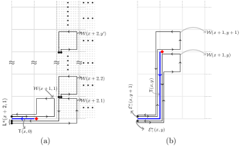
Figure 5: Graphical representation of the inverse canonical relations (III.2.2): a) link electric field $E_{+}^{a}(x,y=0;\hat{1})$, (b) $E_{+}^{a}(x,y\neq 0;\hat{1})$ in terms of plaquette loop operators and loop electric field. The $\bullet$ represents plaquette loop electric fields and $\color[rgb]{1,0,0}\blacklozenge$ represents Kogut-Susskind link electric fields. All loop electric fields $\bullet$ are parallel transported along thick lines to give Kogut Susskind link operator $E^{a}_{+}(x,y;\hat{i})$ or $\color[rgb]{1,0,0}\blacklozenge$ in (III.2.2). In (a) $\sum_{p}{\sf L}^{b}(p)$ gives $\Delta_{X}^{b}(x,y=0)$ in (III.2.2), the summations is over the plaquettes in the dotted region.

The Kogut Susskind link flux operators in terms of the string & loop flux operators are:

$$U(x,y;\hat{1}) = ~{}~{}{\sf T}^{\dagger}(x,y)~{}{\cal W}(x+1,y)~{}{\cal W}(x+1,y-1)$$

$$\cdots\cdots~{}~{}{\cal W}(x+1,1)~{}{\sf T}(x+1,y)$$

$$U(x,y;\hat{2}) = ~{}~{}~{}~{}~{}~{}{\sf T}(x,y+1)~{}{\sf T}^{\dagger}(x,y).$$ (49)

The relations (49) are clear from Figure 2-a,b. The Kogut-Susskind link electric fields in terms of the loop electric fields are (see appendix B for details):

$$E_{+}^{a}(x,y;\hat{1})~{}=~{}R_{ab}({\sf T}^{\dagger}(x,y))\Bigg{[}{\cal E}_{-}^{b}(x+1,y+1)~{}~{}+$$

$$~{}~{}~{}~{}{\cal E}_{+}^{b}(x+1,y)+\underbrace{\delta_{y,0}\sum_{\bar{x}=x+2}^{\sf N}\sum_{\bar{y}=1}^{\sf N}{\sf L}^{b}(\bar{x},\bar{y})}_{\Delta_{X}^{b}(x,y)}\Bigg{]},$$

(50)

$$E_{+}^{a}(x,y;\hat{2})~{}=~{}R_{ab}({\sf T}^{\dagger}(x,y))\bigg{[}{\cal E}_{+}^{b}(x+1,y+1)~{}~{}+$$

$$~{}~{}~{}~{}R_{bc}({\cal W}_{xy}){\cal E}_{-}^{c}(x,y+1)+\underbrace{\sum\limits_{\bar{y}=y+2}^{\sf N}{\sf L}^{b}(x+1,\bar{y})}_{\Delta_{Y}^{b}(x,y)}\bigg{]}.$$

In (III.2.2) we have defined the parallel transport:

$$R_{bc}({\cal W}_{xy})\equiv R_{bc}\big{(}{\cal W}(x,1)~{}{\cal W}(x,2)~{}\cdots{\cal W}(x,y)\big{)}.$$ (51)

and used:  ${\cal E}_{\pm}^{a}(x,y=0)\equiv 0,~{}~{}~{}~{}{\sf L}^{a}(x,y)\equiv\left[{\cal E}^{a}_{-}(x,y)+{\cal E}^{a}_{+}(x,y)\right].$ The inverse relations (III.2.2) and (51) for $E^{a}(x,y=0;\hat{1}),E^{a}(x,y\neq 0;\hat{1})$ and $E^{a}(x,y;\hat{2})$ are illustrated in Figure 5-a,b and Figure 6 respectively. On a single plaquette lattice (III.2.2) reduces to (III.1.1) as expected.

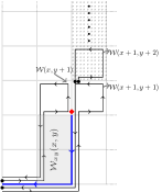
Figure 6: Graphical representation of the inverse canonical relations (III.2.2): $E_{+}(x,y;\hat{2})$ in terms of plaquette loop operators and loop electric field. We show $\Delta_{Y}(x,y)$ where the summation is over the plaquettes in the dotted region. The shaded region represents ${\cal W}_{xy}(x,y)$ in the second equation in (III.2.2).

III.2.3 Physical loop Hilbert space ${\cal H}^{p}$ and Hydrogen atoms

Like in the single plaquette case, the SU(N) Gauss law does not permit any string excitation and the $({\cal N}-1)$ string operators become irrelevant. Therefore, all possible SU(N) gauge invariant operators are made up of the ${\cal P}$ fundamental plaquette loop operators and their conjugate electric fields. In other words, the non-trivial problem of SU(N) gauge invariance over the entire lattice reduces to the problem of residual SU(N) global invariance of $3{\cal P}$ loop operators, all starting and ending at the origin. Further, all $3{\cal P}$ loop operators gauge transform as adjoint matter fields at the origin:

$${\cal W}(p)\rightarrow\Lambda~{}{\cal W}(p)~{}\Lambda^{\dagger},~{}~{}~{}~{}{\cal E}_{\pm}(p)\rightarrow\Lambda~{}{\cal E}_{\pm}(p)~{}\Lambda^{\dagger}.$$ (52)

In (52), $\Lambda=\Lambda(0,0)$ are the gauge transformations at the origin. This global invariance at the origin is fixed by the residual $(N^{2}-1)$ SU(N) Gauss laws:

$${\cal G}^{a}(0,0)=\sum_{p=1}^{\cal P}\Big{[}{\cal E}^{a}_{-}(p)+{\cal E}^{a}_{+}(p)\Big{]}\equiv\sum_{p=1}^{\cal P}~{}{\sf L}^{a}(p)=0.$$ (53)

We now solve the Gauss law (53). A basis in the full Hilbert space of SU(2) lattice gauge theory on a ${\cal P}$ plaquette lattice is given by $\ket{j,m_{-},{m}_{+}}_{1}\otimes\ket{j,m_{-},{m}_{+}}_{2}\otimes\cdots\otimes\ket{j,m_{-},{m}_{+}}_{\cal P}$. We are interested in constructing the physical Hilbert space ${\cal H}^{p}$ which is the $SU(2)$ invariant subspace of the above direct product Hilbert space. As seen in the single plaquette case, it is convenient to define prepotentials for this purpose. We generalize (26) and write:

$${\cal E}_{-}^{a}(p)=a^{\dagger}(p)\left(\frac{\sigma^{a}}{2}\right)a(p),~{}{\cal E}_{+}^{a}(p)=b^{\dagger}(p)\left(\frac{\sigma^{a}}{2}\right)b(p).$$ (54)

We define the number operators on every plaquette: $\hat{N}_{a}(p)\equiv a^{\dagger}(p)\cdot a(p)$ and $\hat{N}_{b}(p)\equiv b^{\dagger}(p)\cdot b(p)$. As the magnitudes of left and right electric field operators are equal we have the following constraint:

$$\hat{N}_{a}(p)=\hat{N}_{b}(p)\equiv\hat{N}(p)$$ (55)

on every plaquette p. The loop flux operators (29) also generalize:

$${\cal W}_{\alpha\beta}(p) = \hat{F}_{p}~{}\Big{[}a_{\alpha}(p)~{}\tilde{b}_{\beta}(p)~{}-~{}\tilde{a}^{\dagger}_{\alpha}(p)~{}b^{\dagger}_{\beta}(p)\Big{]}~{}\hat{F}_{p}$$ (56)

$$\equiv \hat{F}_{p}~{}\Big{[}{\cal W}^{(-)}_{\alpha\beta}(p)~{}+~{}{\cal W}^{(+)}_{\alpha\beta}(p)\Big{]}~{}\hat{F}_{p}.$$

In (56), $\hat{F}_{p}\equiv\frac{1}{\sqrt{(\hat{N}(p)+1)}}$ are the normalization constants so that ${\cal W}$ is unitary. Under SU(2) (global) gauge transformations (52):

$$a_{\alpha}(p)\rightarrow\Lambda_{\alpha\beta}~{}a_{\beta}(p),~{}~{}~{}~{}b_{\alpha}(p)\rightarrow\Lambda_{\alpha\beta}~{}b_{\beta}(p).$$ (57)

In the prepotential representation, we have new U(1) local gauge invariance on each plaquette loop:

$$a_{\alpha}(p)\rightarrow e^{i\theta(p)}~{}a_{\alpha}(p),~{}~{}~{}b_{\alpha}(p)\rightarrow e^{-i\theta(p)}~{}b_{\alpha}(p).$$ (58)

The transformation (58) is generalization of (28). The abelian gauge angle now depends on the location of the plaquette loop. The electric fields (54) and the loop flux operators (56) are invariant under (58). This abelian gauge invariance will play a role later in constructing SO(4,2) loop operators in section (III.2.4). The hydrogen atom states $\ket{{\sf n}_{p}~{}l_{p}~{}m_{p}}$ for each individual plaquette p $(=1,2,\cdots,{\cal P})$ can be constructed exactly like in (31) and (34). Under gauge transformation $\Lambda$ at the origin, all states transform together as:

$$\ket{{\sf n}_{p}~{}l_{p}~{}m_{p}}\rightarrow\sum_{\bar{m}_{p}=-l_{p}}^{l_{p}}D^{~{}~{}l_{p}}_{m_{p}\bar{m}_{p}}\left(\Lambda\right)~{}\ket{{\sf n}_{p}~{}l_{p}~{}\bar{m}_{p}}.$$ (59)

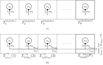
Figure 7: a) Uncoupled and b) Coupled hydrogen atom loop basis. The global Gauss law is solved by putting the total angular momentum ${\sf L}_{\textrm{t}otal}=0$. The tensors involved in the matrix product states in section IV.1.2 are also shown at the bottom. In (a) and (b) $\bullet$ represents the $j$-$j$ coupling or contraction of $j$ flux lines within a plaquette in (34) and in (b) $\otimes$ represents $l$-$l$ couplings or contraction of $l$ flux lines between neighbouring plaquettes (see eqn.(74) and [44]).

Therefore, all principal and angular momentum quantum numbers ${\sf n}_{p},~{}l_{p}$ are already gauge invariant. To proceed further, we separate the gauge variant part of the hydrogen atom state $\ket{{\sf n}~{}l~{}m}$ in (34) from its gauge invariant part on each plaquette. We write it as:

$$\ket{{\sf n}~{}l~{}m}={\sf K}\hat{\cal S}\hat{\cal A}~{}\ket{0}.$$ (60)

In (60), ${\sf K}$ is a normalization constant, $\hat{\cal S}$ and $\hat{\cal A}$ define the symmetric and anti-symmetric parts as follows:

$$\hat{\cal S}\equiv\sum_{\{m_{1}\cdots m_{2l}\}_{m}}\left\{a^{\dagger}_{m_{1}}\cdots a^{\dagger}_{m_{l}}b^{\dagger}_{m_{l+1}}\cdots b^{\dagger}_{m_{2l}}\right\}$$

and

$$\hat{\cal A}\equiv\left(k_{+}\right)^{{\sf n}-l-1}=\left(a^{\dagger}_{1}b^{\dagger}_{2}-a^{\dagger}_{2}b^{\dagger}_{1}\right)^{{\sf n}-l-1}.$$

All magnetic quantum numbers in ${\cal S}$ $m_{1},\cdots,m_{2l}=\pm\frac{1}{2}$ are summed over such that the condition, $m=m_{1}+m_{2}+\cdots+m_{2l}$, is satisfied. In (60), the anti-symmetric operator ${\cal A}\equiv(k_{+})^{{\sf n}-l-1}$ represents the gauge invariant flux loops in (59) within a plaquette. On the other hand, the symmetric operator ${\cal S}\equiv\sum_{\{m_{1}\cdots m_{2l}\}_{m}}\left[a^{\dagger}_{m_{1}}a^{\dagger}_{m_{2}}\cdots a^{\dagger}_{m_{l}}b^{\dagger}_{m_{l+1}}b^{\dagger}_{m_{l+2}}\cdots b^{\dagger}_{m_{2l}}\right]$ represents the uncoupled open flux lines coming out of the plaquette and forming the vector part of the state $\ket{n~{}l~{}m}$. If $l$ has its minimum value $l=0$ on a plaquette then ${\cal S}$ is an identity operator. All $2j~{}(=({\sf n}-1))$ plaquette flux lines are mutually contracted like in the single plaquette case and (60) reduces to (40). This is $j$-$j$ coupling in (34) within a plaquette. At the other limit, if $l$ has its maximum value $l=({\tt n}-1)=2j$ then all $4j$ plaquette loop prepotential operators in (60) are symmetrized and there is no anti-symmetrization or self contraction by $k_{+}$ operator. In other words all $4j$ flux lines flow out of the plaquette and need to be contracted with similar symmetrized flux lines from other plaquettes to get all possible gauge invariant loop states over the entire lattice. This is $l$-$l$ coupling (see [44]). A hydrogen atom state has $0\leq l\leq({\sf n}-1)$. Therefore, it is convenient to represent the hydrogen atom states $\ket{{\sf n}~{}l~{}m}$ by tadpoles on every plaquette as shown in Figure 7-a. The tadpole loop at the top represents the flux flowing in a loop within the plaquette. This is the anti-symmetrized part ${\cal A}$ in (60). The vertical stem of the tadpole is the symmetrized part ${\cal S}$, it represents the flux leakage $(l,m)$ through the plaquette. We now consider the direct product states of all ${\cal P}$ hydrogen atoms in Figure 7-a:

$$\left|\begin{array}[]{cccc}{\sf n}_{1}&{\sf n}_{2}&~{}~{}\cdots~{}~{}~{}{\sf n}_{\cal P}{}{}\\ l_{1}&l_{2}&\cdots~{}~{}~{}l_{\cal P}\\ m_{1}&m_{2}&~{}~{}\cdots~{}~{}m_{\cal P}\end{array}\right\rangle \equiv|{\sf n}_{1}~{}l_{1}~{}m_{1}\rangle\otimes|{\sf n}_{2}~{}l_{2}~{}m_{2}\rangle\cdots$$ (64)

$$\cdots\cdots\otimes|{\sf n}_{p}~{}l_{p}~{}m_{p}\rangle.$$ (65)

In order to solve the Gauss law (53) we describe the states (65) in a coupled basis shown in Figure 7-b. We couple ${\sf L}^{a}_{1},{\sf L}^{a}_{2},\cdots,{\sf L}^{a}_{\cal P}$ and go to a basis where in addition to the diagonal $(J_{1}^{2},J_{2}^{2},\cdots,J_{\cal P}^{2})$ and $({\sf L}_{1}^{2},{\sf L}_{2}^{2},\cdots,{\sf L}_{\cal P}^{2}),$ the following $({\cal P}-3)$ angular momentum operators, commuting with the above two sets, are diagonal:

$$\Bigg{[}({\sf L}_{1}+{\sf L}_{2})^{2},~{}({\sf L}_{1}+{\sf L}_{2}+{\sf L}_{3})^{2},\cdots\cdots,\underbrace{({\sf L}_{1}+{\sf L}_{2}+\cdots{\sf L}_{p})}_{=0~{}({\rm Gauss~{}Law})}{}^{2},$$

$\underbrace{({\sf L}_{1}+{\sf L}_{2}+\cdots+{\sf L}_{p})}_{=0~{}({\rm Gauss~{}Law})}{}^{a=3}\Bigg{]}.$

Note that the total angular momentum is zero implying $({\sf L}_{1}+{\sf L}_{2}+\cdots+{\sf L}_{{\cal P}-1})^{2}={\sf L}^{2}_{\cal P}$ (see Figure 7-b). Thus we have traded off ${\cal P}$ gauge variant magnetic quantum numbers $(m_{1},m_{2},\cdots,m_{\cal P})$ in (65) in terms of $({\cal P}-3)$ gauge invariant eigenvalues of the coupled ${\sf L}$ operators shown above. Therefore, in total there are $3({\cal P}-1)$ members of the complete set of commuting operators. The resulting SU(2) gauge invariant loop basis on a lattice with ${\cal P}$ plaquettes is given by :

$$\left|\begin{array}[]{cccc}{\sf n}_{1}&{\sf n}_{2}&~{}~{}\cdots~{}~{}~{}{\sf n}_{\cal P}{}{}\\ l_{1}&l_{2}&\cdots~{}~{}~{}l_{\cal P}\\ l_{12}&l_{123}&~{}~{}~{}~{}~{}\cdots l_{total}=0\end{array}\right\rangle=\Bigg{\{}|{\sf n}_{1}~{}l_{1}~{}m_{1}\rangle\otimes|{\sf n}_{2}~{}l_{2}~{}m_{2}\rangle$$ (73)

$$\phantom{xxxxxxxxxxxxxxxx}\cdots\otimes|{\sf n}_{p}~{}l_{p}~{}m_{p}\rangle\Bigg{\}}^{{l_{total}=0}}_{{m_{total}=0}}.$$ (74)

Note that, like in the single plaquette case, all topological effects of the compactness of gauge group are now contained in the principal and angular momentum quantum numbers of hydrogen atom $\ket{{\tt n}~{}l~{}m}$. The above loop basis will be briefly denoted by $\left|{\{{\sf n}\}~{}\{l\}~{}\{ll\}}\right\rangle$. The symbols $\{{\sf n}\},~{}\{l\}$ and $\{ll\}$ stand for the sets $({\sf n}_{1},{\sf n}_{2},\cdots,{\sf n}_{\cal P}):{\cal P}$ principal quantum numbers; $~{}(l_{1},l_{2},\cdots,l_{\cal P}):{\cal P}$ angular momentum quantum numbers and $(l_{12},l_{123},\cdots,l_{123\cdots({\cal P}-1)}=l_{\cal P},l_{123\cdots{\cal P}}=0):{\cal P}-3$ coupled angular momentum quantum numbers respectively. These $3({\cal P}-1)$ principal, angular momentum quantum numbers characterizing the loop basis are gauge invariant as is clear from the gauge transformations (59). As expected, this is also the number of physical degree of freedom in the original Kogut-Susskind formulation. In fact, in SU(N) Kogut-Susskind lattice gauge theory in terms of link operators, the total number of physical degrees of freedom is given by the dimension of the quotient space:

$${\mathbb{N}}^{d}_{SU(N)}=\left[\frac{\otimes_{links}~{}SU(N)}{\otimes_{sites}~{}SU(N)}\right]=\left(N^{2}-1\right)\left({\cal L}-{\cal N}\right).$$ (75)

Above, ${\cal L}$ and ${\cal N}$ are the numbers of links and sites of space lattice in d dimension. In $d=2$ we have ${\cal L}-{\cal N}={\cal P}-1$ and if we further choose $N=2$ then, as mentioned above, ${\mathbb{N}}_{SU(2)}$ in (75) is also the number of gauge invariant principal and angular momentum quantum numbers appearing in the orthonormal hydrogen atom loop basis (74) in ${\cal H}^{p}$.

We now discuss pure $SU(N),~{}N\geq 3$ lattice gauge theory in two and three space dimension. A $SU(N)$ tadpole state over a plaquette, analogous to the $SU(2)\otimes SU(2)$ state $\ket{j~{}m}\otimes\ket{j~{}m^{\prime}}\sim\ket{n~{}l~{}m}$ in (31) and illustrated in Figure 7, is characterized by the representations of $SU(N)\otimes SU(N)$ group. These representations or equivalently orthonormal SU(N) tadpole states on each plaquette are labelled by $(N^{2}-1)$ loop quantum numbers . Therefore, in $d=2$ where all ${\cal P}$ plaquette loops are fundamental and mutually independent, there are $(N^{2}-1)~{}{\cal P}$ loop quantum numbers. Subtracting out global $(N^{2}-1)$ degrees of freedom (or gauge transformations at the origin), we again see that there are total $(N^{2}-1)({\cal P}-1)$ gauge invariant SU(N) loop quantum numbers. This exactly matches with ${\mathbb{N}}^{d=2}_{SU(N)}$ in (75) as $({\cal P}-1)=({\cal L}-{\cal N})$ in $d=2$.

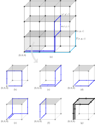
Figure 8: (a) Graphical representation of the fundamental plaquette operators obtained by canonical transformations in $d=3$. The shaded horizontal plaquettes are not obtained by canonical transformations as explained in the text. They are also not independent: the shaded plaquette operator in (g) is the product of the fundamental plaquette loop operators in (b),(c),(d),(e),(f) in that order. This is just the SU(N) Bianchi identity on lattice.

In 3 dimension we repeat $d=2$ canonical transformations on the $z=0$ plane and then extent the string operators ${\sf T}(x,y,z=0)$ in the z directions to construct plaquette loops in $xz$ and $yz$ planes as shown in Figure 8. Thus the canonical transformations already convert all horizontal links on $(xy)$ planes at $z\neq 0$ in forming plaquette loops in the perpendicular $(xz)$ and $(yz)$ planes. Therefore, there are no fundamental $xy$ plaquette loops on $z=1,2,\cdots{\sf N}$ surfaces. These surfaces are shown as shaded planes in Figure 8. In fact, the $(xy)$ plaquette loops at $z\neq 0$ can be written in terms of the fundamental plaquette loops in $(xz)$ and $(yz)$ planes as shown in Figure 8-b,c,d,e,f,g. This way the canonical transformations also bypass the problem of SU(N) Bianchi identity constraints confronted in the loop formulation of SU(N) lattice gauge theories bat in any dimension $d\geq 3$. In $d=3$, we have ${\cal N}=\left({\sf N}+1\right)^{3},~{}{\cal L}=3{\sf N}\left({\sf N}+1\right)^{2}$ and ${\cal P}=3{\sf N}^{2}\left({\sf N}+1\right)$. The total number of $(xy)$ plaquettes is ${\cal P}_{xy}\equiv\frac{\cal P}{3}={\sf N}^{2}(\sf N+1)$. The number of $(xy)$ plaquette at $z=0$ plane is ${\cal P}_{xy}(z=0)=\frac{{\cal P}_{xy}}{\sf N+1}=\sf N^{2}$. Therefore, the number of dependent $(xy)$ plaquettes ${\cal P}_{xy}(z\neq 0)={\cal P}_{xy}-{\cal P}_{(xy)}(z=0)={\sf N}^{3}\equiv$ the number of Bianchi identities. Hence the number of independent SU(N) loop quantum numbers after subtracting $(N^{2}-1)$ gauge degrees of freedom at the origin $=\left(N^{2}-1\right)~{}\left({\cal P}-{\cal P}_{xy}(z\neq 0)-1\right)=\left(N^{2}-1\right)~{}\left({\cal L}-{\cal N}\right)={\mathbb{N}}^{d=3}_{SU(N)}$. This is again an expected result because the canonical transformations used for converting links into (physical) loops & (unphysical) strings can not introduce any spurious degrees of freedom in any dimension. Therefore, the SU(N) plaquette loop operators are mutually independent and contain complete physical information. The corresponding SU(N) coupled tadpole basis is orthonormal as well as complete in ${\cal H}^{p}$ bypassing all non-trivial and notorious SU(N) Mandelstam or Bianchi identity constraints which have been extensively discussed in the past migdal ; bishop ; loll ; rest5 ; manuplb .

III.2.4 Dynamical symmetry group SO(4,2) of hydrogen atom

Having constructed the gauge invariant loop basis in terms of the new plaquette loop operators or in terms of hydrogen atom states in the previous sections, we now discuss the structure of a general gauge invariant operator in ${\cal H}^{p}$. We again illustrate these structures using SU(2) gauge group. In the simplest single plaquette case, we have already seen that the basic $SU(2)$ gauge invariant operators are $\left[k_{0},~{}k_{\pm}\right]$. They (a) are invariant under U(1) gauge transformations (58),  (b) form $SU(1,1)$ algebra and (c) generate transitions $\ket{\sf n}\rightarrow\ket{\bar{\sf n}}$ within the hydrogen atom basis (40) in ${\cal H}^{p}$. We now generalize these three results to the entire lattice in this section. We note that all $4{\cal P}$ loop prepotential operators $\left(a_{\alpha}^{\dagger}(p),~{}a_{\beta}(p)\right)$ and $\left(b^{\dagger}_{\alpha}(p),~{}b_{\beta}(p)\right)$ of the theory transform as matter doublets under SU(2) gauge transformations (57). Therefore, the basic SU(2) tensor operators which are also invariant under U(1) gauge transformations (58) can be classified into the following four classes:

$$\left[a^{\dagger}_{\alpha}(p)b^{\dagger}_{\beta}(p);~{}a_{\alpha}(p)b_{\beta}(p);~{}a^{\dagger}_{\alpha}(p)a_{\beta}(p);~{}b^{\dagger}_{\alpha}(p)b_{\beta}(p)\right].$$ (76)

${\sf L}_{ab}=\epsilon_{abc}\left({\cal E}_{-}^{c}+{\cal E}_{+}^{c}\right)$	$L_{45}=-\frac{i}{2}\big{(}k_{+}-k_{-}\big{)}$	${\sf L}_{a5}=\frac{1}{2}Tr{\sigma_{a}\left({\cal W}^{(+)}-{\cal W}^{(-)}\right)}$
			${\sf L}_{56}=k_{0}$
${\sf L}_{a4}={\left({\cal E}_{-}^{a}-{\cal E}_{+}^{a}\right)}$	$L_{46}=\frac{1}{2}\big{(}k_{+}+k_{-}\big{)}$	${\sf L}_{a6}=\frac{i}{2}Tr{\sigma_{a}\left({\cal W}^{(+)}+{\cal W}^{(-)}\right)}$

Table 1: All possible (15) SU(2) covariant operators on a plaquette which are also U(1) gauge invariant. They form SO(4,2) algebra. We have defined (56)  ${\cal W}^{(+)}_{\alpha\beta}\equiv-\tilde{a}^{\dagger}_{\alpha}b^{\dagger}_{\beta}$ and ${\cal W}^{(-)}_{\alpha\beta}\equiv a_{\alpha}\tilde{b}_{\beta}$.

These are 16 SU(2) gauge covariant and U(1) gauge invariant operators on every plaquette of the lattice. The magnitude of the left and the right electric fields on every plaquette being equal (55), the number operators on each plaquette satisfy $a^{\dagger}(p)\cdot a(p)=b^{\dagger}(p)\cdot b(p)=\hat{N}(p)$. Thus their number reduces to 15. These 15 operators on every plaquette, arranged as in Table 1, form SO(4,2) algebra :

$$\left[L_{AB},L_{CD}\right]=-i~{}\Big{(}g_{AC}~{}L_{BD}~{}+~{}g_{AD}~{}L_{CB}$$

$$+~{}g_{BC}~{}L_{DA}~{}+~{}g_{BD}~{}L_{AC}~{}\Big{)}.$$ (77)

Above, $A,B=1,\cdots,6$ and $g_{AB}$ is the metric $(----++)$. The algebra (77) can be explicitly checked using the prepotential representations of ${\cal E}^{a}_{\mp}$ and ${\cal W}_{\mp}$ in (26) and (29) respectively. Note that the fundamental loop quantization relations (20) are also contained in (77).

In fact, the emergence of SO(4,2) group in SU(2) loop dynamics in the present loop formulation is again an expected result. This can be seen as follows. Let $\ket{\psi}$ be a physical state and $\hat{\cal O}$ be any gauge invariant operator. Then the state $\ket{\psi^{\prime}}\equiv\hat{\cal O}\ket{\psi}$ is also a physical state. As $\ket{\psi},\ket{\psi^{\prime}}\in{\cal H}^{p}$, both can be expanded in the “hydrogen atom loop basis”. We, therefore, conclude that any gauge invariant operator $\hat{\cal O}$ will generate a transition:

$$\ket{{\sf n}~{}l~{}m}~{}~{}\overset{\hat{\cal O}}{\longrightarrow}~{}~{}\sum_{\bar{\sf n},\bar{l},\bar{m}}~{}O_{{\sf n}~{}l~{}m}^{{}^{\bar{\sf n}~{}\bar{l}~{}\bar{m}}}~{}\ket{\bar{\sf n}~{}\bar{l}~{}\bar{m}}.$$

Above, $O_{{\sf n}~{}l~{}m}^{{}^{\bar{\sf n}~{}\bar{l}\bar{~}{}m}}$ are some coefficients depending on the operator $\hat{\cal O}$. On the other hand, any transition $\ket{{\sf n}~{}l~{}m}\rightarrow\ket{\bar{\sf n}~{}\bar{l}~{}\bar{m}}$ can be generated by SO(4,2) generators. This is a very old and well known result in the hydrogen atom literature wyb . Therefore, all gauge invariant operators (including the Hamiltonian in the next section) are SU(2) invariant combinations of these SU(2) covariant and U(1) invariant SO(4,2) generators on different plaquettes of the lattice. These results can also be appropriately generalized to higher SU(N) group by replacing SU(2) prepotential operators by SU(N) irreducible prepotential operators discussed in rmi2 .

IV SU(N) Loop Dynamics

In this section we discuss dynamical issues associated with the SU(N) Kogut-Susskind Hamiltonian after rewriting it in terms of the new fundamental plaquette loop operators. We show that in terms of these plaquette loop operators the initial SU(N) local gauge invariance reduces to global SU(N) invariance and the loop Hamiltonian has a simple weak coupling $g^{2}\rightarrow 0$ continuum limit. The Kogut Susskind Hamiltonian kogut is:

$$H=g^{2}\sum_{l}\vec{E}^{2}_{l}+\frac{K}{g^{2}}\sum_{p}\left(2N-{\textrm{T}r}\left(~{}U_{p}+U_{p}^{\dagger}\right)\right).$$ (78)

In (78) K is a constant, $l\equiv(x,y;\hat{i})$ denotes a link in $\hat{i}$ direction, $p$ denotes a plaquette. The plaquette operator: $U_{p}(x,y)=U(x,y;\hat{1})~{}U(x+1,y;\hat{2})~{}U^{\dagger}(x+1,y+1;\hat{1})~{}U^{\dagger}(x,y+1;\hat{2})$ defines the magnetic field term on a plaquette $p$. As mentioned earlier, we choose space dimension $d=2$. Substituting the Kogut Susskind electric fields in terms of the loop electric fields given in (III.2.2), we get:

$$H = \sum_{x,y\in\Lambda}\Bigg{\{}g^{2}\Big{[}\vec{\cal E}_{-}(x,y)+\vec{\cal E}_{+}(x,y-1)+{\Delta}_{X}(x,y)\Big{]}^{2}$$ (79)

$$+ g^{2}\Big{[}\vec{\cal E}_{+}(x,y)+R\left({\cal W}_{xy}\right)\vec{\cal E}_{-}(x-1,y)+\Delta_{Y}(x,y)\Big{]}^{2}$$

$$+ \frac{K}{g^{2}}\Big{[}2N-{\textrm{T}r}\Big{(}{\cal W}(x,y)+h.c\Big{)}\Big{]}\Bigg{\}}.$$

In (79) all operators vanish when x,y are negative or zero as plaquette loop operators are labelled by top right corner (see Figure 2-a). The operators $\Delta_{X,Y}$ are defined as:

$${\Delta}^{a}_{X}(x,y) \equiv\delta_{y,0}\sum\limits_{\bar{x}=x+1}^{\sf N}\sum\limits_{\bar{y}=1}^{\sf N}~{}{\sf L}(\bar{x},\bar{y}),$$

$${\Delta}^{a}_{Y}(x,y) \equiv~{}~{}~{}~{}\sum\limits_{\bar{y}=y+1}^{\sf N}{\sf L}^{a}(x,\bar{y})$$ (80)

We have also used the relations: $Tr~{}U_{p}(x,y)=Tr\left({\sf T}^{\dagger}(x,y)~{}{\cal W}(x+1,y+1)~{}{\sf T}(x,y)\right)=Tr~{}{\cal W}(x+1,y+1)$. The Hamiltonian (79) describes gauge invariant dynamics directly in terms of the bare essential, fundamental plaquette loop creation and annihilation operators without any gauge fields. As expected, the unphysical strings do not appear in the loop dynamics. There are many interesting and novel features of the Kogut-Susskind Hamiltonian (78) rewritten in terms of loop operators (43):

• There are no local SU(N) gauge degrees of freedom and at the same time there are no redundant loop operators. The $(N^{2}-1)$ residual SU(N) gauge degrees of freedom in (52) can be removed by working in the coupled hydrogen atom basis (74).

• In going from links to loops ((78) to (79)), all interactions have shifted from the magnetic field part to the electric field part. Therefore, the interaction strength now is $g^{2}$ and not $\frac{1}{g^{2}}$. Therefore, the loop Hamiltonian (79) can be used to develop a weak coupling gauge invariant loop perturbation theory near the continuum limit.

• The magnetic field term, dominating in the weak coupling continuum ($g^{2}\rightarrow 0$) limit, acquires its simplest possible form. It creates and annihilates single electric plaquette flux loops exactly like in the single plaquette case (45): $Tr{\cal W}\sim(k_{+}+k_{-})$ with $k_{\pm}\in SU(1,1)\subset SO(4,2)$.

• In the hydrogen atom or tadpole basis (74):

  $$\langle{\sf n}^{\prime}~{}l^{\prime}~{}{m}^{\prime}|H_{B}|{\sf n}~{}l~{}{m}\rangle\equiv\frac{K}{g^{2}}\langle{\sf n}^{\prime}~{}l^{\prime}{m}^{\prime}|Tr{\cal W}|{\sf n}~{}l~{}{m}\rangle$$

  $$~{}~{}~{}~{}~{}~{}~{}~{}=\frac{K}{g^{2}}\delta_{l,l^{\prime}}\delta_{m,m^{\prime}}\left[\delta_{{\sf n}^{\prime},{\sf n}+1}+\delta_{{\sf n}^{\prime},{\sf n}-1}\right].$$ (81)

  In (81) ${\sf n}=2j+1$ and ${\sf n}^{\prime}=2j^{\prime}+1.$ We have ignored the constant and taken $H_{B}\equiv Tr{\cal W}$. If we put $l=0$ in (81), we recover the single plaquette result (46). In fact, the matrix elements (81) in the hydrogen atom loop basis are valid in arbitrary d dimensions. This is in a sharp contrast to the magnetic field term in the standard SU(2) spin network basis leading to (18-j) Wigner coefficients in $d=2$ and (30-j) Wigner coefficient in $d=3$ manuplb .

• The non local terms in the Hamiltonian, ${\Delta}^{a}_{X}(x,y),~{}{\Delta}^{a}_{Y}(x,y)$ and $R({\cal W}_{xy})$ get tamed in the weak coupling limit. In this $g^{2}\rightarrow 0$ limit, the relations (4) imply:

  $${\sf L}^{a}(x,y)={\cal E}^{a}_{-}(x,y)+{\cal E}^{a}_{+}(x,y)\sim 0.$$

  Therefore, ${\Delta}^{a}_{X}(x,y)\sim 0,~{}{\Delta}^{a}_{Y}(x,y)\sim 0$. Further, $R_{ab}({\cal W}_{xy})\sim\delta_{ab}.$ The Hamiltonian, in this weak coupling limit, takes a simple form:

  $$~{}~{}~{}~{}~{}~{}H=\sum\limits_{p=1}^{\cal P}\left\{4g^{2}\vec{\cal E}^{~{}2}(p)+\frac{1}{g^{2}}Tr\left({\cal W}(p)+h.c\right)\right\}~{}+$$ (86)

  $$~{}~{}~{}~{}{g^{2}}\sum_{<pp^{\prime}>}\left\{\vec{\cal E}_{-}(p)\cdot\vec{\cal E}_{+}(p^{\prime})+\vec{\cal E}_{+}(p)\cdot\vec{\cal E}_{-}(p^{\prime})\right\}+g^{3}\delta H.$$

  Above $\sum_{<pp^{\prime}>}$ denotes summation over nearest neighbour plaquette loop electric fields. The non-localities occur in the higher order terms in the coupling. Therefore, these terms, collectively denoted by $g^{3}~{}\delta H$ in (86), can be ignored in the weak coupling limit as a first approximation. The SU(N) gauge theory Hamiltonian in the loop picture now reduces to SU(N) spin model Hamiltonian with nearest neighbour interactions. This simple spin Hamiltonian has the same global SU(N) symmetry, dynamical variables as the Hamiltonian in (79) or (86). In fact, this is an interesting model in its own right to explore confinement and the spectrum in the weak coupling continuum limit. Note that the elementary but dominant $1/g^{2}$ magnetic field terms (see (81)) are left untouched by this approximation. They need to be treated exactly in the $g^{2}\rightarrow 0$ limit and should be part of unperturbed Hamiltonian along with contributions from the electric field terms. As an example, in the simplest case of single plaquette SU(2) lattice gauge theory, the dominant magnetic field term can be easily diagonalized using SU(2) characters robson ; kolawa ; pietri (also see Appendix C). However, it has continuous spectrum (153). Therefore the magnetic field term alone can not be used as unpertubed Hamiltonian even in the weak coupling $(g^{2}\rightarrow 0)$ limit. One has to include contributions from $(g^{2})$ electric field terms in the unperturbed Hamiltonian. These issues are currently under investigation and will be addressed elsewhere.

IV.1 The Schrödinger equation in hydrogen atom loop basis

In this section we explore the ground state $\ket{\Psi_{0}}$ and the first excited state $\ket{\Psi_{1}}$ of SU(2) lattice gauge theory in terms of the SO(4,2) fundamental plaquette loop operators discussed in section III.2.4 and given in Table 1.

IV.1.1 A variational ansatz

An easy, intuitive and old approach is the variational or coupled cluster method greensite . The simple ansatzes are:

$$\ket{\Psi_{0}} = e^{\Gamma}\ket{0},~{}~{}~{}~{}~{}~{}~{}~{}\bra{\Psi_{0}}\Psi_{0}\rangle=1,$$

$$\ket{\Psi_{1}} = \Sigma^{+}~{}\ket{\Psi_{0}},~{}~{}~{}~{}\bra{\Psi_{0}}\Psi_{1}\rangle=0.$$ (87)

In (87) $\Gamma$ and $\Sigma$ are the $SU(2)\otimes U(1)$ gauge invariant operators constructed out of SO(4,2) generators in the Table 1. It is convenient to write $\Gamma=\Gamma^{+}-\Gamma^{-}$ where  $\Gamma^{-}\equiv\left(\Gamma^{+}\right)^{\dagger}$ and $\Gamma^{+},~{}\Sigma^{+}$ have the structures:

$$\Gamma^{+} \equiv G_{1}~{}\sum_{p=1}^{\cal P}k_{+}(p)+\sum_{p_{1},p_{2}=1}^{\cal P}G_{2}(|p_{1}-p_{2}|)\vec{k}_{+}(p_{1})\cdot\vec{k}_{+}(p_{2})$$

$$+ ~{}~{}~{}~{}~{}\cdots\cdots,$$

$$\Sigma^{+} \equiv F_{1}\sum_{p=1}^{\cal P}k_{+}(p)+\sum_{p_{1},p_{2}=1}^{\cal P}F_{2}(|p_{1}-p_{2}|)\vec{k}_{+}(p_{1})\cdot\vec{k}_{+}(p_{2})$$ (88)

$$+ ~{}~{}~{}~{}~{}\cdots\cdots.$$

In the first term above $k_{+}(p)$ is the gauge invariant $SU(1,1)\in SO(4,2)$ plaquette loop creation operator. In the second term, we have defined SU(2) adjoint loop flux creation operator $\vec{k}_{+}(p)$ on every plaquette $p$ using SO(4,2) generators in Table 1:

$$k^{a}_{+}(p)\equiv L_{a5}(p)-iL_{a6}(p)=Tr\left(\sigma^{a}{\cal W}^{(+)}(p)\right),~{}a=1,2,3.$$

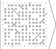
Figure 9: The SU(2) ground state picture in the hydrogen atom basis (74).

Note that the expansion (88) is in terms of number of fundamental loops and not in terms of coupling constant. In fact, $g^{2}$ dependence of the structure functions $G_{1},~{}G_{2},\cdots$ and $F_{1},~{}F_{2},\cdots$ have been completely suppressed. The physical interpretations of (87) and (88) are extremely simple. The operator $e^{\Gamma}$ acting on the strong coupling vacuum in (87) creates loops of all shapes and sizes in terms of the fundamental loop operators to produce the ground state $\ket{\Psi_{0}}$. The first term $k_{+}(p)$ in (88) creates hydrogen atom s-states on plaquette $p$ or simple one plaquette loops. These are shown as small circles (tadpoles without legs) in Figure 9. The second term describes doublets of hydrogen atoms with vanishing total angular momentum. These are shown as two tadpoles joined together in Figure 9. The three hydrogen atom or three tadpole states over three plaquettes ($p_{1},p_{2},p_{3}$) can be created by including a term of the form $\left(\vec{k}_{+}(p_{1})\times\vec{k}_{+}(p_{2})\right)\cdot\vec{k}_{+}(p_{3})$ in $\Gamma^{+}$ and so on and so forth. As shown in Figure 9, the ground state is a soup of all such coupled tadpoles or coupled hydrogen atom clusters, each with vanishing angular momentum. The first excited state in (88) is obtained by exciting loops in this ground state by a creation operator $\Sigma^{+}$. The sizes of the “hydrogen atom clusters” and their importance depend on the structure functions $G$ and $F$ which in turn are fixed by the loop Schrödinger equation with Hamiltonian (86). These qualitative features can be made more precise by putting the ansatz (87) in (86). The resulting Schrödinger equation can be analyzed for the structure constants $(G_{1},~{}G_{2},\cdots)$ and $(F_{1},~{}F_{2},\cdots)$ in the complete, orthonormal hydrogen atom loop basis (74) using its dynamical symmetry group SO(4,2) algebra in (77). We postpone quantitative analysis in this direction to a later publication.

IV.1.2 A tensor networks ansatz

The present loop formulation is tailor-made for tensor network tn6 and matrix product state (MPS) ansatzes to explore the interesting and physically relevant part of ${\cal H}^{p}$ for low energy states. This is due to the following two reasons:

• The absence of non-abelian Gauss law constraints at every lattice site.

• The presence of (spin type) local hydrogen atom orthonormal basis on every plaquette.

We first briefly discuss matrix product state approach in a simple example of spin chain with spin $s=1$ before directly generalizing it to pure SU(2) lattice gauge theory on a one dimensional chain of plaquettes. In the case of spin chain with $s_{x}=-1,0,+1$ at every lattice site $x=0,1,\cdots,N$, any state can be written as:

$$\ket{\Psi}=\sum_{s_{1},s_{2}\cdots s_{N}=0,\pm{1}}\Psi(s_{1},s_{2},\cdots s_{N})\ket{s_{1},s_{2},\cdots s_{N}}.$$ (89)

The matrix product state method consists of replacing the wave functional by

$$\Psi(s_{1},s_{2},\cdots s_{N})=Tr\left(T^{(s_{1})}_{1}T^{(s_{2})}_{2}\cdots T^{(s_{N})}_{N}\right).$$ (90)

In (90) $T^{s}$ are $D\times D$ matrices where D is the bond length. The matrix elements of $T^{s}$ are fixed by minimizing the spin Hamiltonian. In the hydrogen atoms loop basis we have a similar structure where the three dimensional spin states are replaced by infinite dimensional quantum states of hydrogen atoms: $|s\rangle\rightarrow|n~{}l~{}m\rangle$. The most general state in the hydrogen atom loop basis can be written as:

$$\ket{\Psi}=\sum_{\{n\}\{l\}\{m\}}\Psi{\tiny{\left[\begin{array}[]{cccc}n_{1}&n_{2}&\cdots n_{p}\\ l_{1}&l_{2}&\cdots~{}l_{p}\\ m_{1}&m_{2}&~{}\cdots m_{\cal P}\end{array}\right]}}\left|\begin{array}[]{cccc}n_{1}&n_{2}&\cdots~{}n_{p}{}\\ l_{1}&l_{2}&\cdots~{}l_{p}\\ m_{1}&m_{2}&~{}\cdots m_{\cal P}\end{array}\right\rangle.$$ (97)

We now consider SU(2) lattice gauge theory on a chain of ${\cal P}$ plaquettes as shown in Figure 7. A simple tensor network ansatz, like (90 for spins, for the ground state wave function in (97) is

$$\Psi_{0}{\tiny{\left[\begin{array}[]{cccc}n_{1}&n_{2}&~{}~{}\cdots~{}~{}~{}n_{p}{}{}\\ l_{1}&l_{2}&\cdots~{}~{}~{}l_{p}\\ m_{1}&m_{2}&~{}~{}~{}~{}~{}\cdots m_{\cal P}\end{array}\right]}} \equiv Tr\Big{[}T_{1}^{(n_{1}l_{1}m_{1})}~{}T_{2}^{(n_{2}l_{2}m_{2})}\cdots$$ (102)

$$~{}~{}~{}\cdots T_{\cal P}^{(n_{\cal P}~{}l_{\cal P}~{}m_{\cal P})}\Big{]}.$$

In (102) $T_{x}^{(n_{x}l_{x}m_{x})};~{}x=1,2\cdots,{\cal P}$ are ${\cal P}$ matrices of dimension $D\times D$ where $D$ is the bond length describing correlations between hydrogen atoms. Assuming a bound on the principal quantum number (e.g., ${\sf n}=1,2$) and minimizing the energy of the spin model Hamiltonian within spherically symmetric s-sector should give a good idea of ground state at least in the strong coupling region. The method can then be extrapolated systematically towards weak coupling by extending the range of hydrogen atom principal quantum number on each plaquette. The global SU(2) Gauss law can also be explicitly implemented through the following ansatz:

$$\ket{\Psi}=\sum_{\{n\}\{l\}\{ll\}}\Psi{\tiny{\left[\begin{array}[]{cccc}n_{1}&n_{2}&~{}~{}\cdots~{}~{}~{}n_{\cal P}{}{}\\ l_{1}&l_{2}&\cdots~{}~{}~{}l_{\cal P}\\ l_{12}&l_{123}&~{}~{}~{}~{}~{}\cdots l_{12\cdots{\cal P}-2}\end{array}\right]}}~{}~{}~{}~{}~{}~{}~{}~{}~{}~{}~{}~{}~{}~{}~{}~{}~{}~{}~{}~{}$$ (106)

$$~{}~{}~{}~{}~{}~{}~{}~{}~{}~{}~{}~{}~{}~{}~{}~{}~{}~{}~{}~{}~{}~{}~{}~{}~{}~{}~{}~{}\left|\begin{array}[]{cccc}n_{1}&n_{2}&~{}~{}\cdots~{}~{}~{}n_{p}{}{}\\ l_{1}&l_{2}&\cdots~{}~{}~{}l_{p}\\ l_{1}&l_{12}&~{}~{}~{}~{}~{}\cdots l_{12\cdots{\cal P}-2}\end{array}\right\rangle.$$ (110)

We can now make an explicitly gauge invariant MPS ansatz for the ground state:

$$\Psi_{0}{\tiny{\left[\begin{array}[]{cccc}n_{1}&n_{2}&~{}~{}\cdots~{}~{}~{}n_{p}{}{}\\ l_{1}&l_{2}&\cdots~{}~{}~{}l_{p}\\ l_{12}&l_{123}&~{}~{}~{}~{}~{}\cdots l_{12\cdots{\cal P}-2}\end{array}\right]}}\equiv Tr\bigg{[}T^{{}^{~{}n_{1}}}_{{}_{0,l_{1},l_{1}}}(1)~{}T^{{}^{~{}n_{2}}}_{l_{1}l_{2}l_{12}}(2)$$ (114)

$$T^{{}^{~{}n_{3}}}_{l_{12}l_{3}l_{123}}(3)\cdots\cdots T_{l_{\cal P}l_{\cal P}0}^{~{}~{}n_{\cal P}}({\cal P})\bigg{]}.~{}~{}~{}~{}$$ (115)

This ansatz is illustrated in Figure 7-b. Much more work is required to implement these ideas on a computer. We will discuss these computational issues in a future publication.

V Summary and Discussion

In this work we have constructed a series of iterative canonical transformations in pure SU(N) lattice gauge theories to get to a most economical loop formulation without any local spurious degrees of freedom. The canonical transformations ensure that the total degrees of freedom remain intact at every stage. At the end, as a consequence of SU(N) Gauss laws, all local SU(N) gauge degrees of freedom carried by string operators drop out. The loop operators obtained this way are fundamental and the loop formulation is free of difficult SU(N) Mandelstam as well as Bianchi identity ($d\geq 3$) constraints. The resulting SU(N) loop Hamiltonian in two dimension reduces to SU(N) spin Hamiltonian. In the special SU(2) case, the canonical transformations map the physical loop Hilbert space to the space of Wigner coupled hydrogen atoms and the loop dynamics can be completely described in terms of the generators of the dynamical symmetry groups SO(4,2) of hydrogen atoms. Within this loop approach all non-abelian topological effects are contained in the discrete nature of the hydrogen atom energy eigenstates.

We now briefly discuss some new future directions. The absence of SU(N) Gauss laws should help us in defining the entanglement entropy in lattice gauge theories. The entanglement entropy of two complimentary regions in a gauge invariant state suffers from the serious obstacles eent created by SU(N) Gauss laws at the boundary. In the present formulation the two regions can have mutually independent hydrogen atom/tadpole basis which are coupled together across the boundary through a single flux line at the end. The present loop approach may also be interesting in the context of cold atom experiments uca . The hydrogen atom interpretation of ${\cal H}^{P}$ and absence of local gauge invariance should bypass the challenging task of imposing non-trivial and exotic non-abelian Gauss law constraints at every lattice site in the laboratory.

Appendix A From links to loops & strings

In this appendix we generalize the three canonical transformations (11), (14) and (15) in the single plaquette case to the entire lattice in two dimension. We define a comb shaped maximal tree with its base along the $X$ axis and make a series of canonical transformations along the maximal tree to construct the string operators ${\sf T}_{[xxyy]}(x,y)$ attached to each lattice site $(x,y)$ away from the origin. This is similar to the construction of string operators ${\sf T}_{[xy]}(x,y)$ attached to the points $A\equiv(1,0),B\equiv(1,1)$ and $C\equiv(0,1)$ in the simple single plaquette example illustrated in Figure 3-a,b,c. The gauge covariant loop operators ${\cal W}(x,y)$ are constructed by fusing the string operators with the horizontal link operators $U(x,y;\hat{1})$ again through canonical transformations. As expected, all string operators ${\sf T}_{[xxyy]}(x,y)$ decouple as a consequence of SU(N) Gauss laws ${\cal G}^{a}(x,y)=0$. Thus only the fundamental physical loop operators are left at the end. The iterative canonical transformations are performed in 6 steps. These 6 steps are also illustrated graphically in Figures 10-15 for the sake of clarity.

A.1 Strings along x axis

We start by defining iterative canonical transformation along the x axis. They transform the $\sf N$ link operators $U(x,0;\hat{1})$ into $\sf N$ string operators ${{\sf T}}_{[xx]}(x,0)$. These string operators start at the origin and end at $x=1,2,\cdots{\sf N}$ along the x axis as shown in the Figure 10. The canonical transformations are defined iteratively as:

$${\sf T}_{[x]}(x+1,y=0)~{} \equiv~{}{\sf T}_{[x]}(x,0)~{}~{}U(x,0;\hat{1}),$$

$${\sf T}_{[xx]}(x,0)~{} \equiv~{}{\sf T}_{[x]}(x,0),$$

$${\sf E}^{a}_{[x]+}(x+1,0)~{} =~{}E^{a}_{-}(x+1,0;\hat{1}),$$

$${\sf E}^{a}_{[xx]+}(x,0)~{} =~{}E^{a}_{-}(x,0;\hat{1})+E^{a}_{+}(x,0;\hat{1}).$$ (116)

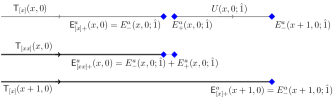
Figure 10: Graphical representation of the iterative canonical transformations (116). The initial ${\sf T}_{[x]}(x,0)$ and the final ${\sf T}_{[xx]}(x,0)$ string operators at $(x,0)$ are shown. The string operator ${\sf T}_{[x]}(x+1,0)$ in the third row replaces ${\sf T}_{[x]}(x,0)$ in the first row in the next iterative step. All electric fields involved in (116) are also shown at their locations.

Above $x=1,\cdots,{\sf N}$ and the starting input for the first equation in (116) is $T_{[x]}(1,0)\equiv U(1,0;\hat{1})$. The canonical transformations (116) iteratively transform the flux operators $\Big{[}{\sf T}_{[x]}(x,0),~{}U(x,0;\hat{1})\Big{]}$ and their electric fields into $\Big{[}{\sf T}_{[xx]}(x,0),~{}{\sf T}_{[x]}(x+1,0)\Big{]}$ and their electric fields as shown in Figure 10. At the boundary $x={\sf N}$, we define ${\sf T}_{[xx]}({\sf N},0)\equiv{\sf T}_{[x]}(\sf N,0)$ for later convenience. As is also clear from Figure 10, the subscript $[xx]$ on the string flux operator ${\sf T}_{[xx]}(x,0)$ encodes the structure of its right electric field ${\sf E}^{a}_{[xx]+}(x,0)$ in (116). More explicitly, the last equation in (116) states that ${\sf E}_{[xx]+}(x,0)$ is the sum of two adjacent Kogut Susskind electric fields in x direction. Note that if we were in one dimension with open boundary conditions, the Gauss law (7) would imply ${\cal G}^{a}(x)\equiv{{\sf T}}^{a}_{[xx]+}(x,0)=0;~{}\forall x$ making all string operators ${\sf T}_{[xx]}(x,0)$ unphysical and irrelevant as expected.

A.2 Strings along y axis

We now iterate the above canonical transformations to extend ${\sf T}_{[xx]}(x,0)$ in the y direction to get ${\sf T}_{[y]}(x,y=1)$ and the final unphysical and ignorable string operators ${\sf T}_{[xxy]}(x,0)$ along the x axis as illustrated in Figure 11:

$${\sf T}_{[y]}(x,1)~{} \equiv~{}{\sf T}_{[xx]}(x,0)~{}U(x,0;\hat{2}),$$

$${\sf T}_{[xxy]}(x,0)~{} \equiv~{}{\sf T}_{[xx]}(x,0)$$

$${\sf E}^{a}_{[y]+}(x,1)~{} =~{}E^{a}_{-}(x,1;\hat{2}),$$

$${\sf E}^{a}_{[xxy]+}(x,0)~{} =~{}{\sf E}^{a}_{[xx]+}(x,0)+E^{a}_{+}(x,0;\hat{2}).$$ (117)

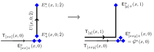
Figure 11: Graphical representation of the canonical transformations (117): vertical string constructions at $y=0$ in (117) and the Gauss law (118) at $y=0$

.

In (117) we have defined ${\sf T}_{[xx]}(0,0)\equiv 1$ and ${\sf T}_{[xx]}({\sf N},0)\equiv{\sf T}_{[x]}({\sf N},0)$ as mentioned above. Substituting ${\sf E}^{a}_{[xx]+}(x,0)$ from (116), we get:

$${\sf E}^{a}_{[xxy]+}(x,0) =\Big{(}{E^{a}_{-}(x,0;\hat{1})+E^{a}_{+}(x,0;\hat{1})+E^{a}_{+}(x,0;\hat{2})}\Big{)}$$

$${\equiv{\cal G}^{a}(x,0)}=0.$$ (118)

Again the subscript $[xxy]$ on the string operator ${\sf T}_{[xxy]}^{a}(x,0)$ denotes that its electric field at $(x,0)$ is sum of three Kogut-Susskind electric fields, two in x direction and one in y direction as in (118) and represented by three squares in Figure 11. We ignore ${\sf T}_{[xxy]}(x,0)$ from now onwards and repeat the canonical transformations (116) to fuse the links in y direction along the maximal tree at fixed $x(=0,1,\cdots{\sf N})$. For this purpose, we replace ${\sf T}_{[x]}(x,0)$ and $U(x,0;\hat{1})$ in (116) by ${\sf T}_{[y]}(x,y)$ and $U(x,y;\hat{2})$ respectively with $y=1,2,\cdots,({\sf N}-1)$ and define:

$${\sf T}_{[y]}(x,y+1)~{} \equiv~{}{\sf T}_{[y]}(x,y)~{}~{}U(x,y;\hat{2}),$$

$${\sf T}_{[yy]}(x,y)~{} \equiv~{}{\sf T}_{[y]}(x,y),$$

$${\sf E}^{a}_{[y]+}(x,y+1)~{} =~{}E^{a}_{-}(x,y+1;\hat{2}),$$

$${\sf E}^{a}_{[yy]+}(x,y)~{} =~{}{{\sf E}}^{a}_{[y]+}(x,y)+E^{a}_{+}(x,y;\hat{2}).$$ (119)

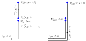
Figure 12: Graphical representation of the canonical transformations (119): iterative vertical string constructions in (119) and the string electric field in (120).

In (119), the initial string operator ${\sf T}_{[y]}(x,y=1)$ is given in (117). The transformations (119) are illustrated in Figure 12. Again the subscript $[yy]$ on ${\sf T}_{[yy]}(x,y)$ is to emphasize that its electric field is sum of two adjacent Kogut Susskind electric fields in the y direction:

$${\sf E}^{a}_{[yy]+}(x,y) ={{\sf E}}^{a}_{[y]+}(x,y)+E^{a}_{+}(x,y;\hat{2})$$

$$={E}^{a}_{-}(x,y;\hat{2})+E^{a}_{+}(x,y;\hat{2}).$$ (120)

In (120) we have used (119) to replace ${\sf E}^{a}_{[y]+}(x,y)$ in terms of Kogut Susskind electric fields $E_{-}^{a}(x,y;\hat{2})$. We again define ${\sf T}_{[yy]}(x,{\sf N})={\sf T}_{[y]}(x,{\sf N})$ at the boundary for notational convenience.

A.3 Plaquette loop operators

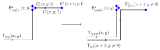
Figure 13: Graphical representation of the canonical transformation in (121).

In order to remove all local SU(N) gauge or string degrees of freedom and simultaneously obtain SU(N) covariant loop flux operators, we now fuse the horizontal link operator $U(x,y\neq 0;\hat{1})$ with ${\sf T}_{[yy]}(x,y\neq 0)$ through the canonical transformations:

$${{\sf T}}_{[x]}(x+1,y) ~{}\equiv~{}{\sf T}_{[yy]}(x,y)~{}U(x,y;\hat{1}),$$

$${\sf T}_{[yyx]}(x,y) ~{}=~{}{\sf T}_{[yy]}(x,y)$$

$${\sf E}_{[x]+}^{a}(x+1,y) ~{}=~{}E^{a}_{-}(x+1,y;\hat{1}),$$

$${\sf E}^{a}_{[yyx]+}(x,y) ~{}=~{}{\sf E}_{[yy]+}^{a}(x,y)+E^{a}_{+}(x,y;\hat{1})$$ (121)

at $x=0,1,2,\cdots,({\sf N}-1)$ and $y=1,2,\cdots,{\sf N}$. The above transformations are illustrated in Figure 13. Using (119), the right electric field of the string flux operator ${\sf T}_{[yyx]}(x,y)$ is:

$${\sf E}^{a}_{[yyx]+} ={\sf E}^{a}_{[yy]+}(x,y)+E^{a}_{+}(x,y;\hat{1})$$

$$=E^{a}_{-}(x,y;\hat{2})+E^{a}_{+}(x,y;\hat{2})+E^{a}_{+}(x,y;\hat{1}).$$ (122)

The initial loop operators $\left(W(x,y),{\mathbb{E}}^{a}(x,y)\right)$ shown in Figure-14 are defined as:

$${W}(x,y) ~{}\equiv~{}{{\sf T}}_{[x]}(x,y\neq 0)~{}{\sf T}^{\dagger}_{[yyx]}(x,y),$$

$${{\sf T}}_{[yyxx]}(x,y) ~{}\equiv~{}{{\sf T}}_{[yyx]}(x,y),$$

$${\mathbb{E}}^{a}_{-}(x,y) ~{}=~{}{\sf E}_{[x]-}^{a}(x,y\neq 0),$$

$${\sf E}^{a}_{[yyxx]+}(x,y) ~{}=~{}{\sf E}^{a}_{[x]+}(x,y\neq 0)+{\sf E}^{a}_{[yyx]+}(x,y).$$ (123)

Above $\left(W(x,y),{\mathbb{E}}^{a}_{\mp}(x,y)\right)$ are canonically conjugate pairs. We note that the conjugate electric fields of the string operators ${\sf T}_{[yyxx]}$ vanishes in ${\cal H}^{p}$ as:

$${\sf E}^{a}_{[yyxx]+}(x,y)~{}=~{}{\sf E}^{a}_{[yyx]+}(x,y)+{\sf E}^{a}_{[x]+}(x,y\neq 0)$$

$$=\Big{(}E^{a}_{-}(x,y;\hat{2})+E^{a}_{+}(x,y;\hat{2})+E^{a}_{+}(x,y;\hat{1})+E^{a}_{-}(x,y;\hat{1})\Big{)}$$

$$={\cal G}^{a}(x,y)=0.$$ (124)

In (124), we have used (121) and (122) to replace ${\sf E}_{[x]+}^{a}(x,y\neq 0)$ and ${\sf E}^{a}_{[yyx]+}(x,y)$ respectively in terms of Kogut-Susskind electric fields. The relationship (124) solving the SU(N) Gauss law at $(x,y)$ is graphically illustrated in Figure 14 and also earlier in Figure 4-a.

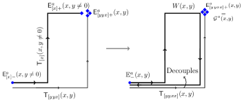
Figure 14: Graphical representation of the canonical transformation in (A.3).

At this stage all the local gauge degrees of freedom, contained in the string operators $T_{[yyxx]}(x,y)$, have been removed. We now relabel ${\sf T}_{[yyxx]}(x,y)$ as ${\sf T}(x,y)$ and ${\sf E}_{[yyxx]\pm}^{a}(x,y)$ as ${\sf E}_{\pm}^{a}(x,y)$ for notational simplicity. To simplify the magnetic field terms in the Kogut Susskind Hamiltonian (42), we further make the last set of canonical transformations (125) which transform the loop operators $(W(x,y),{\mathbb{E}}^{a}_{\pm}(x,y))$ in (A.3) into the final plaquette loop operators $\left({\cal W}(x,y),{\cal E}_{\mp}^{a}(x,y)\right)$ as shown in Figure 15. We define:

$${\cal W}(x,y) ~{}\equiv~{}{W}(x,y-1)~{}\bar{W}^{\dagger}(x,y),$$

$$\bar{W}(x,y-1) ~{}\equiv~{}{W}(x,y-1);$$

$${\cal E}_{+}^{a}(x,y) ~{}=~{}\bar{\mathbb{E}}_{-}^{a}(x,y),$$

$$\bar{\mathbb{E}}_{+}^{a}(x,y-1) ~{}=~{}{\mathbb{E}}_{+}^{a}(x,y-1)+\bar{\mathbb{E}}_{+}^{a}(x,y)$$ (125)

Above $\left[{\cal W}(x,y),{\cal E}_{+}^{a}(x,y)\right],~{}\left[\bar{W}^{\dagger}(x,y),\bar{\mathbb{E}}_{+}^{a}(x,y)\right]$ are canonically conjugate loop operators and $y={\sf N},~{}({\sf N}-1),\cdots,1$. The canonical transformation is initiated with the boundary operator $\bar{W}(x,y={\sf N})\equiv W(x,y={\sf N})$ and at the lower boundary ${\cal W}(x,1)\equiv\bar{W}^{\dagger}(x,1)$.

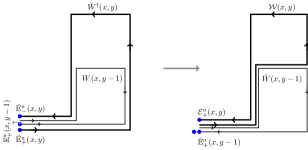
Figure 15: Graphical representation of the canonical transformation in (125).

Having constructed plaquette loop operators and conjugate electric fields using the canonical transformations (121)-(125), we now use these relations to write the plaquette loop electric fields directly in terms of the Kogut-Susskind link electric fields. Using (125),

$${\cal E}_{+}^{a}(x,y)~{} =~{}\bar{{\mathbb{E}}}_{-}^{a}(x,y)=-R_{ab}(\bar{W}(x,y))\bar{\mathbb{E}}_{+}^{a}(x,y)$$

$$=-R_{ab}(\bar{W}(x,y))\left\{\mathbb{E}_{+}^{b}(x,y)+\bar{\mathbb{E}}_{+}^{b}(x,y+1)\right\}$$ (126)

Iterating this relation and using the relation $\mathbb{E}_{+}^{b}(x,y^{\prime})=-R_{bc}(W^{\dagger}(x,y^{\prime}))\mathbb{E}_{-}^{c}(x,y^{\prime})$, we get

$${\cal E}_{+}^{a}(x,y) =-R_{ab}(\bar{W}(x,y))\sum\limits_{y^{\prime}=y}^{{\sf N}}\mathbb{E}_{+}^{b}(x,y^{\prime})$$

$$=R_{ab}({W}(x,y))\sum\limits_{y^{\prime}=y}^{{\sf N}}R_{bc}(W^{\dagger}(x,y^{\prime}))\mathbb{E}_{-}^{c}(x,y^{\prime})$$ (127)

From eqn. (A.3) we have ${\mathbb{E}}_{-}^{c}(x,y^{\prime})={\sf E}_{[x]-}^{c}(x,y^{\prime})=-R_{cd}({\sf T}_{[x]}(x,y^{\prime}))~{}{\sf E}_{[x]+}^{d}(x,y^{\prime})$ and from (121), ${\sf E}_{[x]+}^{d}(x,y^{\prime})=E_{-}^{d}(x,y^{\prime})$. Therefore,

$${\cal E}_{+}^{a}(x,y)=-\sum\limits_{y^{\prime}=y}^{{\sf N}}R_{ab}\left({W}(x,y)W^{\dagger}(x,y^{\prime}){\sf T}_{[x]}(x,y^{\prime})\right)E_{-}^{b}(x,y^{\prime},\hat{1})$$

$$=-\sum\limits_{y^{\prime}=y}^{{\sf N}}R_{ab}\Big{(}{\sf T}(x-1,y)~{}U(x-1,y;\hat{1})~{}\prod_{y^{\prime\prime}=y}^{y^{\prime}}~{}U(x,y^{\prime\prime};\hat{2})\Big{)}$$

$$\phantom{xxxxxxxxxxxxxxxxxxxxxxxxxxxxxxxxxxxxxxx}E_{-}^{b}(x,y^{\prime},\hat{1})$$

$$\equiv-\sum\limits_{y^{\prime}=y}^{{\sf N}}~{}R_{ab}\left(S(x,y,y^{\prime})\right)E_{-}^{b}(x,y^{\prime};\hat{1}).$$ (128)

This is the relation (48) in the text which was further graphically illustrated in Figure 4-b.

Appendix B From loops & strings to links

In this part, we systematically write down all Kogut-Susskind link electric fields in terms of loop flux operators and loop electric fields. We calculate the link electric fields in three separate cases: $a)$ $E^{a}(x,y=0;\hat{1})$ shown in Figure 5-a,  $b)$ $E^{a}(x,y\neq 0;\hat{1})$ shown in Figure 5-b and c) $E^{a}(x,y;\hat{2})$ shown in Figure 6.

B.1 Case (a):  $E_{+}^{a}(x,0;\hat{1})$

Consider the left electric field $E_{+}(x,0;\hat{1})$ of a Kogut Susskind link flux operator $U(x,0;\hat{1})$. From canonical transformation (116) illustrated in Figure 10, we have ${\sf E}_{[xx]+}^{b}(x,0)=E_{-}^{b}(x,0,\hat{1})+E_{+}^{b}(x,0;\hat{1})$. Therefore,

$$E_{+}^{a}(x,0;\hat{1}) =-R_{ab}(U(x,0,\hat{1}))E_{-}^{b}(x+1,0,\hat{1})$$

$$=-R_{ab}(U(x,0,\hat{1}))\left\{{\sf E}_{[xx]+}^{b}(x+1,0)-E_{+}^{b}(x+1,0;\hat{1})\right\}$$ (129)

Iterating this expression, we obtain

$$E_{+}^{a}(x,0;\hat{1}) =R_{ab}\big{(}{\sf T}^{\dagger}(x,0)\big{)}\sum\limits_{{\bar{x}}=x+1}^{{\sf N}}-R_{bc}\left({\sf T}({\bar{x}},0)\right){\sf E}_{[xx]+}^{c}({\bar{x}},0)$$ (130)

Above, we have made use of the fact that ${\sf T}^{\dagger}(x,0){\sf T}(\bar{x},0)=U(x,0;\hat{1})U(x+1,0;\hat{1})\cdots U(\bar{x}-1,0;\hat{1})$ if $\bar{x}>x$. From this expression it is clear that all the $\vec{{\sf E}}_{[xx]+}({\bar{x}},0);{\bar{x}}>x$ are parallel transported back to the point $(x,0)$ to give $\vec{E}_{+}(x,0,\hat{1})$ so that the gauge transformations of link and string operators are consistent with (130). This is a general trend which will be seen at each step of canonical transformations. In fact, the parallel transport is required by the SU(N) gauge transformations of the link and string electric fields in (130). We now convert the string electric fields ${\sf E}^{a}_{[xx]}(x,0)$ into loop electric fields ${\cal E}^{a}(x^{\prime},y^{\prime})$ in three steps.

B.1.1 Converting ${\vec{\sf E}_{[xx]+}\rightarrow\vec{\sf E}_{[y]+}\rightarrow{\vec{\sf E}}_{\bf[yy]+}}$

Writing down $\vec{\sf E}_{[xx]+}(\bar{x},0)$ in terms of $\vec{\sf E}_{[xxy]+}(\bar{x},0)$ and $\vec{\sf E}_{[y]+}(\bar{x},1)$ using canonical transformation 117 shown in Figure 11:

$${\sf E}_{[xx]+}^{a}(\bar{x},0) ={\sf E}_{[xxy]+}^{a}(\bar{x},0)-E_{+}^{a}(\bar{x},0;\hat{2})$$

$$=R_{ab}\left(U(\bar{x},0;\hat{2})\right)\underbrace{E_{-}^{b}(\bar{x},1;\hat{2})}_{{\sf E}_{[y]+}^{b}(\bar{x},1)}$$ (131)

We have used the fact that ${\sf E}_{[xxy]+}(\bar{x},0)=0$ by Gauss law (118) at $(\bar{x},0)$. But from (119) and Figure 12:

$${\sf E}_{[y]+}^{a}(\bar{x},1) ={\sf E}_{[yy]+}^{a}(\bar{x},1)-E_{+}^{a}(\bar{x},1;\hat{2})$$

$$={\sf E}^{a}_{[yy]+}(\bar{x},1)+R_{ab}\left(U(\bar{x},1;\hat{2})\right)\underbrace{E_{-}^{b}(\bar{x},2;\hat{2})}_{{\sf E}_{[y]+}^{b}(\bar{x},2)}$$

$$=R_{ab}\left({\sf T}^{\dagger}(\bar{x},1)\right)\sum_{\bar{y}=1}^{\sf N}R_{bc}\left({\sf T}(\bar{x},\bar{y})\right){\sf E}^{c}_{[yy]+}(\bar{x},\bar{y}).$$ (132)

Substituting it back into eqn. (131) for ${\sf E}_{[xx]+}^{a}(\bar{x},0)$ and using $U(\bar{x},0;\hat{2}){\sf T^{\dagger}}(\bar{x},1)={\sf T^{\dagger}}(\bar{x},0)$, we get

$${\sf E}_{[xx]+}^{a}(\bar{x},0)=R_{ab}\left({\sf T}^{\dagger}(\bar{x},0)\right)\sum_{\bar{y}=1}^{\sf N}R_{bc}\left({\sf T}(\bar{x},\bar{y})\right){\sf E}^{c}_{[yy]+}(\bar{x},\bar{y}).$$ (133)

Putting this into eqn. (130) we get

$$E_{+}^{a}(x,0;\hat{1})=-R_{ab}\big{(}{\sf T}^{\dagger}(x,0)\big{)}\sum\limits_{\bar{x}=x+1}^{\sf N}\sum\limits_{\bar{y}=1}^{\sf N}R_{bc}\left({\sf T}(\bar{x},\bar{y})\right){\sf E}_{[yy]+}^{c}(\bar{x},\bar{y}).$$ (134)

B.1.2 Converting ${\vec{\sf E}_{[yy]+}\rightarrow\vec{\sf E}_{[x]+}\rightarrow\vec{\mathbb{E}}_{\pm}}$

From canonical transformation (121) (Figure 13) we have ${\sf E}_{[yyx]+}^{c}({\bar{x}},{\bar{y}})={\sf E}_{[yy]+}^{c}({\bar{x}},{\bar{y}})+E_{+}^{c}({\bar{x}},{\bar{y}},\hat{1})$ and ${{\sf E}}_{[x]+}^{d}({\bar{x}}+1,{\bar{y}})=E_{-}^{d}({\bar{x}}+1,{\bar{y}},\hat{1})$. Therefore,

$${\sf E}_{[yy]+}^{c}({\bar{x}},{\bar{y}})={\sf E}_{[yyx]+}^{c}({\bar{x}},{\bar{y}})-E_{+}^{c}({\bar{x}},{\bar{y}},\hat{1})$$

$$={\sf E}_{[yyx]+}^{c}({\bar{x}},{\bar{y}})+R_{cd}\left(U({\bar{x}},{\bar{y}},\hat{1})\right)\underbrace{E_{-}^{d}({\bar{x}}+1,{\bar{y}},\hat{1})}_{{{\sf E}}_{[x]+}^{d}({\bar{x}}+1,{\bar{y}})}$$ (135)

Further, the canonical transformations (A.3) (Figure 14) imply:

$${\sf E}_{[yyx]+}^{c}({\bar{x}},{\bar{y}})={\sf E}_{[yyxx]+}^{c}({\bar{x}},{\bar{y}})-{{\sf E}}_{[x]+}^{c}({\bar{x}},{\bar{y}})=-{{\sf E}}_{[x]+}^{c}({\bar{x}},{\bar{y}})$$

Here, we have used the fact that ${\sf E}_{[xxyy]+}^{c}({\bar{x}},{\bar{y}})=0$ by Gauss law at $(\bar{x},\bar{y})$ (eqn. (124)). Also, from eqn. (A.3), ${\sf E}_{[x]-}^{d}(\bar{x},\bar{y})={\mathbb{E}}_{-}^{d}({\bar{x}},{\bar{y}})$. Therefore,

$${{\sf E}}_{[x]+}^{c}({\bar{x}},{\bar{y}}) =-R_{cd}({{\sf T}}^{\dagger}_{[x]}({\bar{x}},{\bar{y}})){{\sf E}}_{[x]-}^{d}({\bar{x}},{\bar{y}})$$

$$=-R_{cd}({{\sf T}}^{\dagger}_{[x]}({\bar{x}},{\bar{y}})){\mathbb{E}}_{-}^{d}({\bar{x}},{\bar{y}})$$ (136)

Substituting for $\vec{\sf E}_{[yyx]+},\vec{\sf E}_{[x]+}$ in eqn. (135) and using the relation $U({\bar{x}},{\bar{y}};\hat{1}){\sf T}^{\dagger}_{[x]}({\bar{x}}+1,{\bar{y}})={\sf T}^{\dagger}({\bar{x}},{\bar{y}})$,

$${\sf E}_{[yy]+}^{c}({\bar{x}},{\bar{y}}) =R_{cd}\left({{\sf T}}^{\dagger}_{[x]}({\bar{x}},{\bar{y}})\right){\mathbb{E}}_{-}^{d}({\bar{x}},{\bar{y}})$$

$$-R_{cd}\left({\sf T}^{\dagger}({\bar{x}},{\bar{y}})\right){\mathbb{E}}_{-}^{d}({\bar{x}}+1,{\bar{y}})$$ (137)

Putting (137) in (134) and using the defining relations

$${\sf T}(\bar{x},\bar{y}){\sf T}^{\dagger}_{[x]}(\bar{x},\bar{y})\equiv{W}^{\dagger}(\bar{x},\bar{y});$$

$${\mathbb{E}}_{+}^{b}(\bar{x},\bar{y})\equiv-R_{bd}\left({W}^{\dagger}(\bar{x},\bar{y})\right){\mathbb{E}}_{-}^{d}(\bar{x},\bar{y}).$$

we get a simple relation:

$$E^{a}_{+}(x,0;\hat{1}) =R_{ab}\big{(}{\sf T}^{\dagger}(x,0)\big{)}$$

$$\sum\limits_{\bar{x}=x+1}^{\sf N}~{}\sum\limits_{\bar{y}=1}^{\sf N}~{}\Big{[}{\mathbb{E}}_{+}^{b}(\bar{x},\bar{y})+{\mathbb{E}}_{-}^{b}(\bar{x}+1,\bar{y})\Big{]}.$$ (138)

B.1.3 Converting ${\vec{\mathbb{E}}_{\pm}\rightarrow\vec{\cal E}_{\pm}}$

To write ${E}_{+}^{a}(x,0;\hat{1})$ in terms of the final plaquette loop electric fields ${\cal E}_{\pm}^{b}$, we first use the canonical transformation in equation (125) and shown in Figure 15: ${\mathbb{E}}_{+}^{b}(\bar{x},\bar{y})=\bar{{\mathbb{E}}}_{+}^{b}(\bar{x},\bar{y})-\bar{{\mathbb{E}}}_{+}^{b}(\bar{x},\bar{y}+1)$. This enables us to write down the first term in the eqn. (138) in terms of $\vec{\cal E}_{-}$ as follows:

$$\sum\limits_{\bar{y}=1}^{\sf N}{\mathbb{E}}_{+}^{b}(\bar{x},\bar{y}) =\sum\limits_{\bar{y}=1}^{\sf N}\left[\bar{{\mathbb{E}}}_{+}^{b}(\bar{x},\bar{y})-\bar{{\mathbb{E}}}_{+}^{b}(\bar{x},\bar{y}+1)\right]=\bar{{\mathbb{E}}}_{+}^{b}(\bar{x},1)$$

$$=-R_{bc}\left(\bar{W}^{\dagger}(\bar{x},1)\right)\bar{{\mathbb{E}}}^{c}_{-}(\bar{x},1)$$

$$=-R_{bc}\left(\mathcal{W}(\bar{x},1)\right){\mathcal{E}}_{+}^{c}(\bar{x},1)={\mathcal{E}}_{-}^{b}(\bar{x},1).$$ (139)

Here, we have used the fact that at the lower boundary, $\bar{W}^{\dagger}(\bar{x},1)=\mathcal{W}(\bar{x},1)$. We now write down the second term in eqn.(138) in terms of $\vec{\cal E}_{\pm}$. Again using canonical transformation eqn.(125) (Figure 15) as follows:

$${\mathbb{E}}_{-}^{b}({\bar{x}}+1,{\bar{y}})=-R_{bc}(\bar{W}({\bar{x}}+1,{\bar{y}})){\mathbb{E}}_{+}^{c}({\bar{x}}+1,{\bar{y}})$$

$$=-R_{bc}(\bar{W}({\bar{x}}+1,{\bar{y}}))\left[\bar{{\mathbb{E}}}_{+}^{c}({\bar{x}}+1,{\bar{y}})-\bar{{\mathbb{E}}}^{c}_{+}({\bar{x}}+1,{\bar{y}}+1)\right]$$

$$=\bar{{\mathbb{E}}}_{-}^{b}({\bar{x}}+1,{\bar{y}})-R_{bc}\big{(}\bar{W}({\bar{x}}+1,{\bar{y}})\bar{W}^{\dagger}({\bar{x}}+1,{\bar{y}}+1)\big{)}\bar{{\mathbb{E}}}^{c}_{-}({\bar{x}}+1,{\bar{y}}+1)$$

$$=\bar{{\mathbb{E}}}_{-}^{b}({\bar{x}}+1,{\bar{y}})-R_{bc}({\mathcal{W}}({\bar{x}}+1,{\bar{y}}+1))\bar{{\mathbb{E}}}^{c}_{-}({\bar{x}}+1,{\bar{y}}+1)$$

$$={\mathcal{E}}_{+}^{b}({\bar{x}}+1,{\bar{y}})+{\mathcal{E}}_{-}^{b}({\bar{x}}+1,{\bar{y}}+1)$$ (140)

Putting both the terms back into eqn. (138) for $E_{+}^{a}(x,0;\hat{1})$, we get

$$E_{+}^{a}(x,0;\hat{1})=R_{ab}\big{(}{\sf T}^{\dagger}(x,0)\big{)}$$

$$\sum\limits_{{\bar{x}}=x+1}^{{\sf N}}\left\{{\mathcal{E}}_{-}^{b}({\bar{x}},1)+\sum\limits_{{\bar{y}}=1}^{{\sf N}}\left[{\mathcal{E}}_{+}^{b}({\bar{x}}+1,{\bar{y}})+{\mathcal{E}}_{-}^{b}({\bar{x}}+1,{\bar{y}}+1)\right]\right\}$$

$$=R_{ab}\big{(}{\sf T}^{\dagger}(x,0)\big{)}\bigg{\{}{\mathcal{E}}_{-}^{b}(x+1,1)+\sum\limits_{{\bar{x}}=x+2}^{{\sf N}}\sum\limits_{{\bar{y}}=1}^{{\sf N}}{\sf L}^{b}({\bar{x}},{\bar{y}})\bigg{\}}$$ (141)

Above, ${\sf L}^{a}(\bar{x},\bar{y})\equiv{\cal E}_{-}^{a}(\bar{x},\bar{y})+{\cal E}_{+}^{a}(\bar{x},\bar{y})$.

B.2 Case (b): $E_{+}^{a}(x,y\neq 0;\hat{1})$

The canonical transformation (121) and Figure 13 state that ${{\sf E}}_{[x]+}^{b}(x,y)=E_{-}^{b}(x,y;\hat{1})$. Therefore,

$$E_{+}^{a}(x,y,\hat{1}) =-R_{ab}(U(x,y,\hat{1}))~{}E_{-}^{b}(x+1,y;\hat{1})$$

$$=-R_{ab}(U(x,y,\hat{1}))~{}{{\sf E}}_{[x]+}^{b}(x+1,y)$$ (142)

Using the relations (136) and (140)

$${{\sf E}}_{[x]+}^{b}(x+1,y)=-R_{bc}({{\sf T}}^{\dagger}_{[x]}(x+1,y)~{}{\mathbb{E}}_{-}^{c}(x+1,y);$$

$${\mathbb{E}}_{-}^{c}(x+1,y)={\mathcal{E}}_{+}^{c}(x+1,y)+{\mathcal{E}}_{-}^{c}(x+1,y+1)$$ (143)

and relation ${\sf T}^{\dagger}(x,y)=U(x,y,\hat{1}){{\sf T}}^{\dagger}_{[x]}(x+1,y)$ , we get

$$E_{+}^{a}(x,y,\hat{1}) =\left[R_{ab}(U(x,y,\hat{1}))R_{bc}({{\sf T}}^{\dagger}_{[x]}(x+1,y))\right]{\mathbb{E}}_{-}^{c}(x+1,y)$$

$$=R_{ac}\left({\sf T}^{\dagger}(x,y)\right){\mathbb{E}}_{-}^{c}(x+1,y)$$

$$=R_{ac}\left({\sf T}^{\dagger}(x,y)\right)\bigg{\{}{\mathcal{E}}_{+}^{c}(x+1,y)+{\mathcal{E}}_{-}^{c}(x+1,y+1)\bigg{\}}$$ (144)

Clubbing case (a) and case (b) together,

$$E_{+}^{a}(x,y;\hat{1})=R_{ab}({\sf T}^{\dagger}(x,y))$$

$$\bigg{(}{\cal E}_{-}^{b}(x+1,y+1)+{\cal E}_{+}^{b}(x+1,y)+\delta_{y,0}\sum_{\bar{x}=x+2}^{\sf N}\sum_{\bar{y}=1}^{{\sf N}}{\mathbb{L}}^{b}(\bar{x},\bar{y})\bigg{)}.$$ (145)

We have defined ${\cal E}_{\pm}(x,0)\equiv 0;~{}{\cal E}_{\pm}(0,y)\equiv 0$ for notational convenience. The relations (141) were used in (III.2.2) and (79), (80) to write down the Kogut Susskind Hamiltonian in terms of loop operators.

B.3 Case (c):  $E_{+}(x,y;\hat{2})$

The canonical transformations (119) (Figure 12) state ${\sf E}_{[y]+}^{c}(x,y)=E_{-}^{c}(x,y,\hat{2})$. Therefore,

$$E_{+}^{a}(x,y;\hat{2}) =-R_{ac}\left(U(x,y;\hat{2})\right)E_{-}^{c}(x,y+1,\hat{2})$$

$$=-R_{ac}\left(U(x,y;\hat{2})\right){\sf E}_{[y]+}^{c}(x,y+1)$$ (146)

Using the relation ${\sf E}_{[y]+}^{c}(x,y)={\sf E}_{[yy]+}^{c}(x,y)-E_{+}^{c}(x,y,\hat{2})$ from the canonical transformation eqn. (119) (Figure 12),

$$E_{+}^{a}(x,y;\hat{2})=-R_{ac}(U(x,y,\hat{2}))\left\{{\sf E}_{[yy]+}^{c}(x,y+1)-E_{+}^{c}(x,y+1,\hat{2})\right\}$$

$$=-R_{ac}(U(x,y,\hat{2})){\sf E}_{[yy]+}^{c}(x,y+1)$$

$$-R_{ac}\left(U(x,y,\hat{2})U(x,y+1,\hat{2})\right){\sf E}_{[yy]+}^{c}(x,y+2)-\cdots$$

$$=-R_{ab}({\sf T}^{\dagger}(x,y))\sum\limits_{{\bar{y}}=y+1}^{\sf N}R_{bc}\left({\sf T}(x,\bar{y})\right)~{}{\sf E}_{[yy]+}^{c}(x,\bar{y})$$ (147)

Using eqn.(137), ${\sf E}_{[yy]+}^{c}(x,\bar{y})=R_{cd}\left({\sf T}^{\dagger}_{[x]}(x,\bar{y})\right)~{}{\mathbb{E}}_{-}^{d}(x,\bar{y})-R_{cd}\left({\sf T}^{\dagger}(x,\bar{y})\right)~{}{\mathbb{E}}_{-}^{d}(x+1,\bar{y})$ and the expression $W^{\dagger}(x,\bar{y})={\sf T}(x,\bar{y}){\sf T}^{\dagger}_{[x]}(x,\bar{y})$ from eqn. (A.3),

$$E_{+}^{a}(x,y;\hat{2}) =R_{ab}\left({\sf T}^{\dagger}(x,y)\right)$$

$$\sum\limits_{{\bar{y}}=y+1}^{\sf N}\left[-R_{bc}\left(W^{\dagger}(x,\bar{y})\right){\mathbb{E}}_{-}^{c}(x,\bar{y})+{\mathbb{E}}_{-}^{b}(x+1,\bar{y})\right].$$ (148)

From eqn. (140), we have ${\mathbb{E}}_{-}^{c}(x,\bar{y})={\mathcal{E}}_{+}^{c}({x},{\bar{y}})+{\mathcal{E}}_{-}^{c}({x},{\bar{y}}+1)$. Therefore, ${\mathbb{E}}_{-}^{b}(x+1,\bar{y})={\mathcal{E}}_{+}^{b}({x+1},{\bar{y}})+{\mathcal{E}}_{-}^{b}({x+1},{\bar{y}}+1)$ and

$$\sum\limits_{{\bar{y}}=y+1}^{\sf N}-R_{bc}\left(W^{\dagger}(x,\bar{y})\right)~{}{\mathbb{E}}_{-}^{c}(x,\bar{y})$$

$$=\sum\limits_{{\bar{y}}=y+1}^{\sf N}-R_{bc}\left(W^{\dagger}(x,\bar{y})\right)\Big{[}{\mathcal{E}}_{+}^{c}({x},{\bar{y}})+{\mathcal{E}}_{-}^{c}({x},{\bar{y}}+1)\Big{]}$$

$$=\sum\limits_{{\bar{y}}=y+1}^{\sf N}\Big{\{}R_{bc}\left(W^{\dagger}(x,\bar{y}-1)\right){\mathcal{E}}_{-}^{c}({x},{\bar{y}})$$

$$\phantom{xxxxxxxxxx}-R_{bc}\left(W^{\dagger}(x,\bar{y})\right){\mathcal{E}}_{-}^{c}({x},{\bar{y}}+1)\Big{\}}$$

$$=R_{bc}\left(W^{\dagger}(x,y)\right){\mathcal{E}}_{-}^{c}({x},{y+1})$$ (149)

Above, we have used the relations: $W^{\dagger}(x,\bar{y})=W^{\dagger}(x,\bar{y}-1)~{}{\cal W}(x,\bar{y})$ and $R_{cd}\left({\cal W}(x,\bar{y})\right){\cal E}_{+}^{d}(x,\bar{y})={\cal E}_{-}^{c}(x,\bar{y})$. Putting these two terms back into eqn. (148),

$$E_{+}^{a}(x,y;\hat{2})= R_{ab}\left({\sf T}^{\dagger}(x,y)\right)\Bigg{\{}R_{bc}\left({W}^{\dagger}(x,y)\right){\mathcal{E}}_{-}^{c}(x,y+1)$$

$$~{}+\sum\limits_{{\bar{y}}=y+1}^{{\sf N}}\left[{\mathcal{E}}_{+}^{b}(x+1,{\bar{y}})+{\mathcal{E}}_{-}^{b}(x+1,{\bar{y}}+1)\right]\Bigg{\}}$$ (150)

Therefore,

$$E_{+}^{a}(x,y;\hat{2}) =R_{ab}({\sf T}^{\dagger}(x,y))\bigg{(}{\cal E}_{+}^{b}(x+1,y+1)$$

$$+R_{bc}({{\cal W}_{xy}(x,y)}){\cal E}_{-}^{c}(x,y+1)+\sum\limits_{\bar{y}=y+2}^{{\sf N}}{\sf L}^{b}(x+1,\bar{y})\bigg{)}$$ (151)

Above, ${\cal W}_{xy}(x,y))\equiv{\cal W}(x,1){\cal W}(x,2)\cdots{\cal W}(x,y)$ as defined in (51). The relation (151) was stated in (III.2.2) and used later in (79) to get the SU(N) loop Hamiltonian.

Once the string operators decouple from the theory (as shown in the previous section), the only remaining or residual Gauss law is at the origin. This Gauss law at the origin states:

$$E_{+}^{a}(0,0;\hat{1})+E_{+}^{a}(0,0;\hat{2})=0.$$

When rewritten in terms of the plaquette electric fields using the above relations (145) and (151) it takes the form:

$$\sum\limits_{{x},{y}=1}^{{\sf N}}{\sf L}^{a}({x},{y})~{}=~{}0.$$

This is the residual SU(N) Gauss law at the origin.

Appendix C Mathieu equation

We now exploit the simple action of the magnetic field term on the hydrogen atom basis (46) to construct the dual magnetic basis where this magnetic term is diagonal. We define $\ket{j}\equiv\ket{\tt n}_{\tt n\equiv 2j+1}$ and

$$\ket{\omega}=\sum_{j}~{}\chi_{j}(\omega)~{}\ket{j}.$$ (152)

In (152), $\chi_{j}(\omega)=\frac{sin\left(2j+{1}\right)\frac{\omega}{2}}{sin\left(\frac{\omega}{2}\right)}$ are the SU(2) characters. Using the recurrence relations varshalovich :

$$\chi_{j+\frac{1}{2}}(\omega)+\chi_{j-\frac{1}{2}}(\omega)=2cos\left(\frac{\omega}{2}\right)\chi\left(\omega\right),$$

we get

$$H_{B}\ket{\omega}=~{}\frac{1}{g^{2}}~{}\left(Tr{\cal W}\right)~{}\ket{\omega}=~{}\frac{2}{g^{2}}~{}cos\left(\frac{\omega}{2}\right)~{}\ket{\omega}.$$ (153)

Note that $\omega$ is a gauge invariant angle. We now use the differential equation of the SU(2) character varshalovich :

$$\frac{d^{2}\chi_{j}}{d\omega^{2}}+cot\left(\frac{\omega}{2}\right)\frac{d\chi_{j}(\omega)}{d\omega}+j(j+1)\chi_{j}(\omega)=0$$

to convert $H_{E}$ in (40) into differential operator in $\omega$. Finally the Schrödinger equation $H\ket{\psi}_{\epsilon}=\epsilon\ket{\psi}_{\epsilon}$ in this gauge invariant loop basis is the Mathieu equation:

$$\Big{[}\frac{d^{2}}{d\omega^{2}}+\frac{1}{4}\Big{]}\phi_{\epsilon}(\omega)+\frac{\kappa}{4}\Big{[}\epsilon-2\kappa\left(1-cos\left(\frac{\omega}{2}\right)\right)\Big{]}\phi_{\epsilon}\left(\omega\right)=0.$$ (154)

In (154) we have defined $\kappa\equiv\frac{1}{g^{2}}$ and $\phi_{\epsilon}(\omega)\equiv sin\frac{\omega}{2}~{}\psi_{\epsilon}(\omega)$ where $~{}\psi_{\epsilon}(\omega)\equiv\langle\omega|\psi\rangle_{\epsilon}$. The Mathieu equation (154) and its discrete solutions has been extensively discussed in the past in the context of single plaquette lattice gauge theory bishop ; robson ; kolawa ; mathieu .

References

- (1) K. G. Wilson, Phys. Rev. D 10 (1974) 2445.
- (2) S. Mandelstam, Phys. Rev. 175 (1968) 1580; S. Mandelstam, Phys. Rev. D 19 (1979) 2391.
- (3) T. T. Wu, C. N. Yang, Phys. Rev. D 12 (1975) 3845.
- (4) Y. Nambu, Phys. Letts. B 80 (1979) 372.
- (5) A. M. Polyakov, Nucl. Phys. B 164 (1979) 171.
- (6) J. Kogut, L. Susskind, Phys. Rev. D 11 (1975) 395.
- (7) J. Goldstone, R. Jackiw, Phys. Letts. B 74, 81 (1978).
- (8) F. A. Lunev, Phys. Letts. B 295 (1992) 99-103 ; Michel Bauer, Daniel Z. Freedman, Peter E. Haagensen, Nuclear Physics B 428 (1994) 147-168; P. E. Haagensen, K. Johnson, Nuclear Physics B 439 (1995) 597-616; P. E. Haagensen, K. Johnson, C. S. Lam, Nuclear Physics B 477 (1996) 273-292.
- (9) P. Majumdar, H. S. Sharatchandra, Physics Letters B 491 (2000) 199-202 ; I. Mitra and H. S. Sharatchandra, arXiv:1307. 0989 (2013).
- (10) R. Anishetty, P. Majumdar, H. S. Sharatchandra, Physics Letters B 478 (2000) 373-378 ; R. Anishetty, Phys. Rev. D 44, 1895 (1991).
- (11) D. Karabali, V. P. Nair, Nuclear Physics B 464 (1996) 135-152; V. P. Nair, A. Yelnikov, Nucl. Phys. B 691 (2004) 182 ; L. Freidel, R. G. Leigh, and D. Minic, Phys. Lett. B 641 (2006) 105.
- (12) R. Gambini, Jorge Pullin, Loops, Knots, Gauge Theories and Quantum Gravity (Cambridge University Press, 2000).
- (13) Y. M. Makeenko, A. A. Migdal, Nucl. Phys. B 188 (1981) 269; A. Jevicki, B. Sakita, Phys. Rev. D 22 (1980) 467; B. Brügmann, Phys. Rev. D 43 (1991) 566; Gambini R, Leal L, Trias A, Phys. Rev. D 39 (1989) 3127; Bartolo C, Gambini R, Leal L, Phys. Rev. D 39 (1989) 1756.
- (14) R. Loll, Nucl. Phys. B 368 (1992) 121 ; R. Loll, Nucl. Phys. B 400 (1993) 126; Watson N. J. , Phys. Letts. B 323 (1994) 385; N. J Watson, Nucl. Phys. Proc. Suppl. 39 B (1995) 224, hep-th/9408174.
- (15) A. A. Migdal, Phys. Rep. 102(1983) 199; V. F Muller, W. Ruhl, Nucl. Phys. B 230 (1984) 49;
- (16) N. E. Ligterink, N. R. Walet, R. F. Bishop, Ann of phys. 284 (2000) 215.
- (17) M. Mathur, Nuclear Physics B 779 (2007) 32-62. M. Mathur, Phys. Lett. B 640 (2006) 292-296;
- (18) H. S. Sharatchandra, Nucl. Phys. B 196 (1982) 62; R. Anishetty, H. S. Sharatchandra, Phys. Rev. Letts. 65 (1990) 813; R. Anishetty, I. Raychowdhury, Phys. Rev. D 90 (2014) 114503.
- (19) D. Robson, D. M. Webber, Z. Phys. C 15 (1982) 199.
- (20) W. Furmanski, A. Kolawa, Nucl. Phys. B 291 (1987) 594.
- (21) G. Burgio, R. De Pietri, H.A. Morales-Tecotl, L.F. Urrutia, J.D. Vergara, Nucl.Phys. B566 (2000) 547-561.
- (22) M. Mathur, J. Phys. A 38 (2005) 10015-10026.
- (23) M. Mathur, T. P. Sreeraj, Phys. Lett. B 749 (2015) 137.
- (24) R. Anishetty, M. Mathur, I. Raychowdhury, J. Phys. A 43 (2010) 035403; M. Mathur, I. Raychowdhury, R. Anishetty , J. Math. Phys. 51, 093504 (2010).
- (25) F. Girelli, E. R. Livine, Class. Quant. Grav. 22 (2005) 3295-3314; N. D. Hari Dass, M. Mathur, 24 (2007) 2179-2192;
- (26) C. Rovelli, Quantum Gravity, Cambridge University Press (2004); C. Rovelli, L. Smolin, Phys. Rev. D 52 (1995) 5743.
- (27) A. Ashtekar, Phys. Rev. Letts. 57 (1986) 2244.
- (28) G. G. Batrouni, Nucl. Phys. B 208 (1982) 467; O. Borisenko, S. Voloshin , M. Faber, Nucl. Phys. B 816 (2009) 399; J. Kiskis, Phys. Rev. D 26 (1982) 429 .
- (29) B. G. Wybourne, Classical group for physicists, John Wiley and sons (1974); R. Gilmore, Lie Groups, Physics and Geometry, Cambridge University Press (2008). M. Bander and C. Itzykson, Group Theory and the Hydrogen Atom (I), Rev. Mod. Phys. 38 (1966) 330.
- (30) J. Greensite, Nucl. Phys. B 166 (1980) 113; Schütte D, Weihong Z, Hamer C J, Phys. Rev. D 55 (1997) 2974; H. Arisue, M. Kato and T. Fujiwara, Prog. Theor. Phys, 70 (1983) 229; P. Suranyi, Nucl. Phys. B210 (1982), 519;
- (31) S. Östlund, S. Rommer, Phys. Rev. Lett 75 (1995) 3537; I. McCulloch, J. Stat. Mech. : Theory Exp. P10014 (2007); F. Verstraete, V. Murg, J. I. Cirac, Advances in Physics, 57:2 (2008) 143-224; S. Singh, G. Vidal, Phys. Rev. B 86 (2012) 195114 ;
- (32) A. Milsted, arXiv:1507. 06624v1 (2015) (and references therein).
- (33) H. Casini, M. Huerta, and J. A. Rosabal, Phys. Rev. D 89 (2014) 085012; S. Aoki, T. Iritani, M. Nozaki, T. Numasawa, N. Shiba, H. Tasaki, arXiv:1502. 04267 (2015).
- (34) E. Zohar, J. I. Cirac, B. Reznik, arXiv:1503. 02312 [quant-ph] (and references therein). E. Zohar, E. Cirac, B Reznik, Phys. Rev. A 88 (2013) 023617; K. Stannigel, P. Hauke, D. Marcos, M. Hafezi, S. Diehl, M. Dalmonte, P. Zoller, Phys. Rev. Lett. 112 (2014) 120406; L. Tagliacozzo, A. Celi, P. Orland, M. Lewenstein, Nature Commun. 4 (2013) 2615 .
- (35) D. A. Varshalovich, A. N. Moskalev and V. K. Khersonskii, Quantum Theory of Angular Momentum (World Scientific 1988).
- (36) D. Robson, D. M. Webber, Z. Phys. C 7 (1980) 53; R. F. Bishop, A. S. Kendall, L. Y. Wong, and Y. Xian, Phys. Rev. D 48 (1993) 887 ; E. Dagotto and A. Moreo, Phys. Rev. D 31 (1985) 865.