Spin Orbit Coupling in Graphene Induced by Heavy Adatoms with Electrons in the Outer-Shell $p$ Orbitals.

Abstract

Many of the exotic properties proposed to occur in graphene rely on the possibility of increasing the spin orbit coupling (SOC). By combining analytical and numerical tight binding calculations, in this work we study the SOC induced by heavy adatoms with active electrons living in $p$ orbitals. Depending on the position of the adatoms on graphene different kinds of SOC appear. Adatoms located in hollow position induce spin conserving intrinsic like SOC whereas a random distribution of adatoms induces a spin flipping Rashba like SOC. The induced SOC is linearly proportional to the adatoms concentration, indicating the inexistent interference effects between different adatoms. By computing the Hall conductivity we have proved the stability of the topological quantum Hall phases created by the adatoms against inhomogeneous spin orbit coupling . For the case of Pb adatoms, we find that a concentration of 0.1 adatom per carbon atom generates SOC’s of the order of $\sim$40$meV$.

I Introduction

The research on graphene, a two-dimensional crystal of carbon atoms, has driven to the discover of a large number of interesting electrical, magnetic, mechanical and optical propertiesCastro Neto et al. (2009); M.I.Katsnelson (2012). The small atomic number of carbon implies that electrical carriers in graphene have a extremely weak spin-orbit (SO) couplingHuertas-Hernando et al. (2006); Min et al. (2006). This property in combination with the large graphene electron mobility makes graphene a very good candidate for using in spintronicsDlubak et al. (2012); Chico et al. (2015).

On the other hand some proposasl of exotic topological phases in graphene rely on the possibility of increasing the SOC. Because of the graphene lattice symmetry, there are two types of spin orbit coupling in graphene, intrinsic-like, where the ${\hat{z}}$-component of the electron spin is a good quantum number and ${\it Rashba}$-like which mixes spins and appears in absence of mirror symmetryKane and Mele (2005). In graphene, the intrinsic SOC opens a gap and the system becomes a quantum spin Hall insulator, with gapless edge states able to transport spin and chargeHasan and Kane (2010); Qi and Zhang (2011). Non-trivial topological phases may also occur in multilayer graphene Prada et al. (2011). Quantum anomalous Hall effect was predicted to occur in bilayer and monolayer graphene in presence of Rashba SOC and an exchange field or magnetic impuritiesQiao et al. (2010); Tse et al. (2011). The experimental realization of these topological phases requires a large SOC, and therefore there is a big interestCastro Neto and Guinea (2009); Abdelouahed et al. (2010); Chico et al. (2009); Gosálbez-Martinez et al. (2011); Balakrishnan et al. (2013); Calleja et al. (2015); Avsar et al. (2014) in increasing the SOC and clear the way to the study of exotic topological phases in graphene. Experimental reports on enhancement of SOC in graphene by weak hydrogenationBalakrishnan et al. (2013), gold hybridizationMarchenko et al. (2012) or proximity with WS₂Avsar et al. (2014), indicate that it is possible to increase the SOC in almost three orders of magnitude. Recently, it has been reported that graphene grown on Cu shows a SO splitting around 20 meVBalakrishnan et al. (2014). Intercalation of Au atoms in graphene grown on Ni produces a SO splitting of near 100meVMarchenko et al. (2012). Similarly, the intercalation of Pb atoms in graphene grown on a iridium substrate seems to produce a giant SOCCalleja et al. (2015). Theoretically, it has been proposed that heavy adatoms with partially filled $p$-shells, deposited on symmetric positions of the graphene lattice, could induce large intrinsic SOCWeeks et al. (2011).

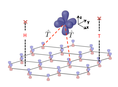
Figure 1: (Color online)Schematic representation of the effective hopping between carbon atoms induced by an adatom with active electrons in outer $p$-shells. Vertical, H and T, lines indicate the hollow and top positions respectively

In this work we study the SOC induced by heavy adatoms with active electrons living in p-orbitals, in particular we consider Pb atoms, that have been proved to induce large SO effects in grapheneCalleja et al. (2015).

The physical picture is the following, the tunneling of an electron between two carbon atoms through the adatoms $p$-orbitals opens new channels for hopping in graphene. The SOC between the adatom $p$ orbitals makes that the new tunneling channels can conserve the spin inducing a intrinsic SOC or can flip the spin inducing a Rashba like SOC.

By combining analytical calculations, perturbation theory and tight-binding based numerical simulations, we study the type of SO coupling induced by adatoms residing in different positions of the graphene unit cell. In addition, we study how a finite density of adatoms, in different distributions, affects the induced SO couplings. The main conclusions of our work are the following,

i) adatoms located in hollow positions, see Fig.1, induce intrinsic SOC. A finite density of adatoms in hollow positions opens an energy gap at the Dirac points, that increases linearly with the adatom concentration. This gapped phase is a quantum spin Hall state. The simulations indicate that, even for high adatom coverage, there are not interference effects between the adatoms and the gap only depends on adatom density. In the case of Pb atoms we find gaps of the order of 50meV for a concentration of 0.1 adatom per carbon.

ii) for adatoms placed in top positions, see Fig.1, the tunneling from graphene to the adatom and back, induces a Rashba like spin flip hopping between the underneath C atom and its first neighbors and an intrinsic like spin conserving second neighbors tunneling between the carbons surrounding the underneath carbon atom. The intrinsic like SOC induced by adatoms in top positions has opposite sign than the induced by adatoms in hollow geometry. The Rashba SOC has the same sign independently of the sublattice of the underneath carbon.

iii) A finite density of adatoms randomly distributed on graphene, induces a finite Rashba SOC linearly proportional to the density of adatoms. For a random distribution of adatoms, the resulting intrinsic like SOC vanishes, because contributions from different locations of the adatoms have opposite signs. Similar results are obtained when the adatoms form an array commensurate with a large graphene supercell. By computing the Hall conductivity, we have obtained that a random distribution of adatoms on graphene in presence of an exchange field, is an anomalous quantum Hall system. When the adatom is Pb, we obtain that the Rashba SO coupling can be as larger as 35meV for a concentration of 0.1 Pb per carbon atom.

The rest of the paper is organized in the following way, in Section II we introduce the graphene and adatom Hamiltonians, and in Section III we describe the hopping between graphene carbon atoms and the adatom p-orbitals. In Section IV we present the perturbation theory for describing the adatom mediated effective hopping between carbon atoms. The knowledge of the effective hopping between carbon atoms allow us to obtain, in Section V, analytical expressions for SOC induced by adatoms located in top and hollow positions. Section VI turns to present tight-binding based numerical simulations for studying the effect that a random or commensurate distribution of adatoms have on the induced SOC. In Section VII we calculate the topological properties of graphene doped with adatoms. We close the paper with a summary of the results.

II Preliminaries.

II.1 Graphene Hamiltonian

In graphene, carbon atoms crystallize in a triangular lattice of primitive translation vectors ${\bf a}$=$(0,a)$ and ${\bf b}$=$(\sqrt{3}/2,1/2)a$, where $a$=2.46Å is the lattice constant. The positions of the triangular lattices are ${\bf R}_{i}$. There are two atoms per unit cell located at positions ${\bf d}_{A}$=$(0,0)$ and ${\bf d}_{B}$=$(a/\sqrt{3},0)$, that define sublattices $A$ and $B$ in graphene. Covalent $sp_{2}$ bonds between carbon atoms stabilize this honeycomb lattice whereas the tunneling between $p_{z}$ orbitals is the origin of the low energy active conduction and valence $\pi$-bands. The band structure is rather well described by a tight-binding model with hopping $t\sim 2.7$eV between first neighbors carbon $p_{z}$ orbitals,

$$H_{0}=-t\sum_{<i_{A},i_{B}>,\sigma}\left(|Z,i_{A},\sigma><Z,i_{B},\sigma|+H.c.\right)$$ (1)

Here the sum runs over first neighbors pairs and $|Z,i_{\alpha},\sigma>$ represents the wavefunction of an electron at position ${\bf R}_{i}$+${\bf d}_{\alpha}$ occupying a carbon $p_{z}$ orbital with $z$-component of the spin $\sigma$. The energy of the $p_{z}$ carbon orbital is chosen as the zero of energies.

In graphene the intrinsic SOC has a chiral structure of the form,

$$H_{SO}^{I}\!=\!\lambda^{SO}\!\!\!\!\!\!\!\!\sum_{<i_{\alpha},j_{\alpha}>,\sigma}\!\!\!\!\left(i\sigma(\hat{\bf u}_{i_{\alpha}}\!\times\!\hat{\bf u}_{j_{\alpha}})_{z}|Z,i_{\alpha},\sigma\!><\!Z,j_{\alpha},\sigma|\!+\!H.c.\right)$$ (2)

where the sum runs over second nearest neighbors carbon atoms and $\hat{\bf u}_{i_{\alpha}}$ is a unit vector parallel to $\bf R_{i}$+${\bf d}_{\alpha}$. Note that the intrinsic SOC conserves spin and it is not associated with broken mirror symmetry. On the contrary, Rashba SOC appears because of broken mirror symmetry, in particular due to the substrate, and induces a coupling between first neighbors with opposite spin of the form,

$$H_{SO}^{R}\!=\!i\lambda^{R}\!\!\!\!\!\!\!\!\!\!\sum_{<i_{A},j_{B}>,\sigma,\sigma^{\prime}}\!\!\!\!\!\!\left((\boldsymbol{\sigma}\!\times\!\hat{\bf u}_{i_{A}j_{B}})_{z}|Z,i_{A},\sigma\!><\!Z,j_{B},\sigma^{\prime}|+H.c.\right)$$ (3)

here $\hat{\bf u}_{i_{\alpha}j_{\beta}}$ is a unit vector parallel to ${\bf R}_{j}+{\bf d}_{\beta}-{\bf R}_{i}-{\bf d}_{\alpha}$ and $\boldsymbol{\sigma}$ the electron spin Pauli matrices.

In absence of SO couplings the conduction and valence bands touch at two inequivalent points of the Brillouin zone ${\bf K}$=$(0,\frac{4\pi}{3a})$ and ${\bf K}^{\prime}$=$(0,-\frac{4\pi}{3a})$ which are the celebrated Dirac points. Near these points the low energy physics is described by the Dirac equation

$$H_{0}=\hbar v_{F}(k_{x}\sigma_{0}\otimes\tau_{x}+sk_{y}\sigma_{0}\otimes\tau_{y})\,$$ (4)

here the moment $\bf{k}$ is measured with respect the Dirac points, $s$=1 and -1 stands for ${\bf K}$ and $\bf K^{\prime}$ respectively, and $\boldsymbol{\tau}$ are the Pauli matrices acting on the spinor defined by the amplitude of the wave function on sublattices $A$ and $B$. In the previous equation $\sigma_{0}$ represents the unity matrix in the spin sector. The Fermi velocity is related with the hopping trough the relation $\hbar v_{F}$=$\frac{\sqrt{3}}{2}ta$. In this continuum approximation the SO terms get the form,

$$H_{SO}^{I} = 3\sqrt{3}\lambda^{SO}s\,\sigma_{z}\otimes\tau_{z}$$ (5)

$$H_{SO}^{R} = \frac{3}{2}\lambda^{R}(s\,\sigma_{x}\otimes\tau_{y}-\sigma_{y}\otimes\tau_{x})\,.$$ (6)

II.2 Adatom Hamiltonian.

We consider heavy atoms with the active electrons living in $p$ orbitals. The Hamiltonian describing the electrons in the adatom contains a spin-orbit coupling part and a crystal field $H_{CF}$ term. In the basis$\{|p_{x}\uparrow>,|p_{y}\uparrow>,|p_{z}\uparrow>,|p_{x}\downarrow>,|p_{y}\downarrow>,|p_{z}\downarrow>\}$ the Hamiltonian reads,

$$H_{p}=\Delta_{SO}{\bf L}\cdot{\boldsymbol{\sigma}}+H_{CF}=$$

$$\frac{\Delta_{SO}}{2}\!\left(\!\begin{array}[]{cccccc}0&-i&0&0&0&1\\ i&0&0&0&0&-i\\ 0&0&0&-1&i&0\\ 0&0&-1&0&i&0\\ 0&0&-i&-i&0&0\\ 1&i&0&0&0&0\end{array}\!\right)\!\!+\!\!\left(\!\begin{array}[]{cccccc}\epsilon_{x}&0&0&0&0&0\\ 0&\epsilon_{y}&0&0&0&0\\ 0&0&\epsilon_{z}&0&0&0\\ 0&0&0&\epsilon_{x}&0&0\\ 0&0&0&0&\epsilon_{y}&0\\ 0&0&0&0&0&\epsilon_{z}\end{array}\!\right)\,\,.$$ (19)

Here $\Delta_{SO}$ is the spin-orbit coupling parameter, ${\bf L}$ and ${\boldsymbol{\sigma}}$ are the usual angular momentum and spin operators. Non spherical effects occurring in the geometry produce a crystal field that splits the energies of the $p$ orbitals. For adatoms deposited on planar graphene, we expect that $\epsilon_{x}$=$\epsilon_{y}\neq\epsilon_{z}$.

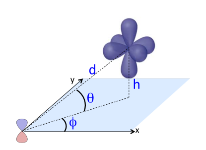
Figure 2: (Color online)Geometry of and adatom located at a distance $h$ of the graphene layer. The angles $\theta$ and $\phi$ and the distance $d$ define the spherical coordinates of the adatom with respect to a carbon atom.

III Tunneling between an adatom and a carbon $Z$ orbital.

We consider an adatom placed at position ${\bf r}$=$(x,y,h)$, where $h$ is the vertical distance between graphene and the adatoms, Fig.2. The tunneling amplitudes between an carbon orbital located at position ${\bf R}_{i}$=$(X_{i},Y_{i},0)$, and the adatom $p_{x}$, $p_{y}$ and $p_{z}$ orbitals are,

$$<Z,i,\sigma|\hat{T}|p_{x},\sigma> = \frac{1}{2}\cos\phi\sin{2\theta}(V_{pp\sigma}(d)\!-\!V_{pp\pi}(d))$$

$$<Z,i,\sigma|\hat{T}|p_{y},\sigma> = \frac{1}{2}\sin\phi\sin{2\theta}(V_{pp\sigma}(d)\!-\!V_{pp\pi}(d))$$

$$<Z,i,\sigma|\hat{T}|p_{z},\sigma> = \cos^{2}\theta V_{pp\pi}(d)+\sin^{2}\theta V_{pp\sigma}(d)$$ (20)

where $\theta$=$\tan^{-1}\frac{h}{\sqrt{(x-X_{i})^{2}+(y-Y_{i})^{2}}}$, $\phi$=$\tan^{-1}\frac{y-Y_{i}}{x-X_{i}}$, and $V_{pp\sigma}$ and $V_{pp\pi}$ are the Slater-Koster hopping parameters between the $p_{z}$ graphene orbital and the heavy adatom $p$-orbitals. The hopping parameters depend on the distance $d$=$\sqrt{(x-X_{i})^{2}+(y-Y_{i})^{2}+h^{2}}$ between the atoms, that we parametrize in the form, $V_{pp\sigma(\pi)}(d)$=$V_{pp\sigma(\pi)}(d=h)e^{-\beta(d-h)}$ with $\beta$=3Suárez Morell et al. (2011) and $V_{pp\sigma(\pi)}(h)$ obtained from density functional calculationsCalleja et al. (2015). Note that in the tunneling process the carrier spin is conserved. Because of the symmetry of the $p$-orbitals, the hopping amplitude between a carbon $p_{z}$-orbital in graphene and the $p_{x}$ and $p_{y}$ adatom orbitals, have opposite sign depending weather the adatom is deposited on top or bottom of the graphene sheet. On the contrary, the hopping between $z$-orbitals is independent of the position of the adatom with respect the graphene layer.

IV Tunneling between carbon atoms mediated by an adatom.

The spin-orbit coupling in the adatom located at ${\bf r}$=$(x,y,h)$, allows an extra path for tunneling between two carbon atoms located at ${\bf R}_{i}$ and ${\bf R}_{j}$ with spin $\sigma$ and $\sigma^{\prime}$ respectively. In second order perturbation theory a single adatom produces a coupling between the carbon atoms of the form,

$$\gamma_{i\sigma,j\sigma^{\prime}}=\sum_{l}\frac{<Z,i,\sigma|\hat{T}|\,\tilde{p}_{l}><\tilde{p}_{l}\,|\hat{T}|Z,j,\sigma^{\prime}>}{\tilde{\epsilon}_{l}}$$ (21)

here $|\tilde{p}_{l}>$ and $\tilde{\epsilon}_{l}$ are the eigenfunctions and eigenvalues of Hamiltonian Eq.19. Because of the form of spin-orbit coupling in the adatom outer $p$ shell, the induced hoppings satisfy the following relations for $i\neq j$

$$\gamma {}_{i\sigma,j-\sigma}=-\gamma^{*}_{i-\sigma,j\sigma}$$ (22)

$$\gamma {}_{i\sigma,j\sigma}=\gamma^{*}_{i-\sigma,j-\sigma}$$

$$\gamma {}_{i\sigma,j\sigma^{\prime}}=\gamma^{*}_{j\sigma^{\prime},i\sigma}$$

and for $i=j$

$$\gamma {}_{i\sigma,i\sigma}=\gamma_{i-\sigma,i-\sigma}$$ (23)

$$\gamma {}_{i\sigma,i-\sigma}=0$$ (24)

The adatom gives rise to two kind of SO assisted tunneling,

i) spin conserved tunneling events of the form

$$|Z,i,\sigma\!>\stackrel{{\scriptstyle\hat{T}}}{{\longrightarrow}}|p_{x(y)}\sigma\!>\stackrel{{\scriptstyle H_{p}}}{{\longrightarrow}}|p_{y(x)}\sigma\!>\stackrel{{\scriptstyle\hat{T}}}{{\longrightarrow}}|Z,j,\sigma\!>$$ (25)

that are pure imaginary and change sign when reversing spin. Following the standard notation we call it intrinsic spin-orbit coupling. This tunneling amplitude behaves as $\sin^{2}(2\theta)$, it is zero when the adatom is in the graphene sheet, being independent on the top or bottom position of the adatom with respect the graphene layer.

ii) non-conserving spin processes of the form

$$| Z ,i,\sigma\!\!>\stackrel{{\scriptstyle\hat{T}}}{{\longrightarrow}}|p_{z}\sigma\!\!>\stackrel{{\scriptstyle H_{p}}}{{\longrightarrow}}|p_{x(y)}-\sigma\!\!>\stackrel{{\scriptstyle\hat{T}}}{{\longrightarrow}}|Z,j,-\sigma\!\!>$$

$$| Z ,i,\sigma\!\!>\stackrel{{\scriptstyle\hat{T}}}{{\longrightarrow}}|p_{x(y)}\sigma\!\!>\stackrel{{\scriptstyle H_{p}}}{{\longrightarrow}}|p_{z}-\sigma\!\!>\stackrel{{\scriptstyle\hat{T}}}{{\longrightarrow}}|Z,j,-\sigma\!\!>$$ (26)

These terms get origin on the lack of mirror symmetry in the hopping between $z$-orbitals and we refer to this tunneling contribution as Rashba SOC. This tunneling amplitude behaves as $\sin(2\theta)$ and changes sign when the adatom is located on top or on bottom of the graphene layer.

V Effective Hamiltonians for Hollow and Top Positions

When the adatoms are located at high symmetry points of the graphene lattice, it is possible to write down analytic expressions for the effect that the SO induces on the graphene low energy band structure. The procedure consist in projecting the perturbation created by the adatom on the atomic Bloch states at the ${\bf K}$ and ${\bf K^{\prime}}$ Dirac points,

$$\Psi_{A,s,\sigma} = \frac{1}{\sqrt{N}}\sum_{i}e^{is{\bf K}{\bf R}_{i}}|Z,i_{A},\sigma>$$

$$\Psi_{B,s,\sigma} = \frac{1}{\sqrt{N}}\sum_{i}e^{is{\bf K}{\bf R}_{i}}|Z,i_{B},\sigma>\,,$$ (27)

here $N$ is the number of of unit cells in the crystal. These Bloch states are the eigenstates of the Dirac Hamiltonian, Eq.4 for ${\bf k}$=0. We assume that adatoms do not induce coupling between states coming from different Dirac cones. We have checked numerically this assumption, provided the adatoms do not form a periodic array with a reciprocal lattice vector equal to ${\bf K-\bf K^{\prime}}$.

V.1 Adatom in Hollow Position

In the hollow geometry the adatom is located on top of the center of an hexagon of the graphene lattice at a height $h$, see Fig.1. We consider SO induced tunneling up to third neighbors, tunneling between more distant atoms can be neglected because of the exponential decreasement of the tunneling amplitude with the distance. Coupling between Bloch wavefunctions of different sublattices involves first and third neighbors hopping and gets the form

$$<\Psi_{A,s,\sigma}|V_{H}|\Psi_{|B,s,\sigma^{\prime}}>=\frac{1}{N}\sum_{i_{A},j_{B}}\gamma_{i_{A}\sigma,j_{B}\sigma^{\prime}}e^{is{\bf K}({\bf R}_{j}-{\bf R}_{i})}$$ (28)

here $i_{A}$ ($j_{B}$) runs over the vertices, of sublattice $A$ ($B$), of the hexagon surrounding the adatom. $V_{H}$ represents the perturbation created by the adatom in hollow position.

The coupling between Bloch states of the same sublattice involves second neighbors tunneling and gets the form,

$$<\Psi_{A,s,\sigma}|V_{H}|\Psi_{|A,s,\sigma^{\prime}}>=\frac{1}{N}\sum_{i_{A}\neq j_{A}}\gamma_{i_{A}\sigma,j_{A}\sigma^{\prime}}e^{is{\bf K}({\bf R}_{j}-{\bf R}_{i})}.$$ (29)

Similar expression applies for $<\Psi_{B,s,\sigma}|V_{H}|\Psi_{|B,s,\sigma^{\prime}}>$. The adatom also induces diagonal selfenergies that for the adatom in the hollow position are equal for both Dirac points, spin orientation and graphene sublattices.

In the hollow geometry and for $\sigma^{\prime}$=$-\sigma$, it is possible to sum the six terms, Eq.26, that contribute to spin flip effective tunneling, and we get

$$\gamma_{i\sigma,j-\sigma}=-\sigma t_{R}\left(e^{-i\sigma\phi_{j}}-e^{-i\sigma\phi_{i}}\right)$$ (30)

being $t_{R}$ a constant that depends on the carbon to adatom tunneling parameters, Eq.20. Using this expression and relations Eq.22 we obtain that in the hollow position an adatom with outer shell $p$ orbitals does not induce non-conserving spin tunneling and therefore does not induce Rashba like SOC in graphene.

For spin conserving SO induced tunneling, the sum of the two processes described in Eq.25, gives a hopping,

$$\gamma_{i\sigma,j\sigma}=i\sigma t_{so}\sin\left(\phi_{i}-\phi_{j}\right)$$ (31)

where $t_{so}$ is a constant that depends on the distance between the adatom and the graphene sheet. When introducing this hopping and applying the symmetries Eq.22, we obtain that the coupling between Bloch states of different sublattices and same spin cancels identically. On the contrary the spin conserving coupling between same sublattice Bloch functions gets a finite value that changes sign when changing spin, sublattice or Dirac cone,

$$<\Psi_{\tau,s,\sigma}|V_{H}|\Psi_{\tau,s,\sigma}>=\frac{1}{N}3\sqrt{3}t_{so}\,\sigma\,s\,\tau\,.$$ (32)

This term has the same form than the Hamiltonian Eq.6 and we conclude, in agreement with reference Weeks et al. (2011), that an heavy adatom, with electrical active $p$-orbital, in a hollow position on top of graphene induces an intrinsic like SOC.

V.2 Adatom in Top Position

In this geometry the adatom is located vertically on top of a carbon atom at a height $h$. This configuration privileges the sublattice $A$ of the underneath carbon atom. In the top arrangement the carbon $p_{z}$ orbital is orthogonal to the $p_{x}$ and $p_{y}$ orbitals of the adatom located on top of it. Therefore the processes contributing to first neighbors spin conserving tunneling are zero by symmetry, Eq.25. However, an adatom on top of a carbon of a given sublattice, induces spin conserving tunneling between carbon atoms of the opposite sublattice,

$$<\!\Psi_{B(A),s,\sigma}|V_{T_{A(B)}}|\Psi_{B(A),s,\sigma}\!>=\tau_{A(B)}\frac{3\sqrt{3}}{N}t_{so}\,\sigma\,s,$$ (33)

here $V_{T_{A(B)}}$ represents the perturbation created by the adatom on top of atoms belonging to sublattice $A(B)$. Therefore adatoms in top positions induce intrinsic-like SO coupling, although it is important to note that the sign of this conserving tunneling is opposite to the induced by an adatom in hollow position, Eq.32

Because of the symmetry of the orbitals, only one of the mechanisms described in Eq.26 contributes to spin flip tunneling between first neighbors,

$$\gamma_{i\sigma,j-\sigma}=-\sigma t_{R}e^{-i\sigma\phi_{j}}\,,$$ (34)

where $t_{R}$ is a constant that depends on carbon to adatom tunneling parameters. Adding the contributions from the three first neighbors of the underneath C atom, we get the following contribution to the low energy Hamiltonian,

$$<\Psi_{A,s,\sigma}|V_{T_{A(B)}}|\Psi_{B,s,-\sigma}>=\frac{1}{N}3t_{R}\,s\,\frac{(1+\sigma\,s)}{2}\,\,.$$ (35)

This Rashba like SOC has the same form and sign independently on the sublattice where the adatom is placed. The Rashba term gets its origin in the broken mirror symmetry produced by the adatoms and this is reflected in that $t_{R}$ change sign depending whether the top adatoms are located on top or bottom of the graphene layer.

VI Numerical results.

Adatoms deposited on graphene should be placed at minimum energy equilibrium positions. The adsorption geometry depends on the particular heavy adatomWeeks et al. (2011), being one of the more interesting that in which the adatoms place in hollow positions. When the adatoms are intercalated between graphene and the substrate, the adatoms form a superlattice commensurated with the graphene honeycomb latticeCalleja et al. (2015). It is also plausible to expect that low energy injected adatoms become deposited in random positions.

In this Section we show numerical results of the electronic structure of graphene doped with heavy outer shell $p$-orbitals adatoms in three particular cases, i) the adatoms are randomly distributed in hollow positions, ii) the adatoms form a commensurate supercell with the graphene lattice and iii) the adatoms are fully random distributed on the graphene sheet.

In the numerical calculations we consider a periodic rectangular graphene supercell of dimensions $L_{x}$=$N_{x}\sqrt{3}a$ and $L_{y}$=$N_{y}a$, defined by the lattice vectors, A=$N_{y}{\bf a}$ and B = $N_{x}(2{\bf b}-{\bf a})$. In these expressions $N_{x}$ and $N_{y}$ are integer numbers. The unit cell contains 4$N_{x}N_{y}$ carbon atoms located at the graphene lattice positions $\{{\bf R}_{i}+{\bf d}_{\alpha}\}$. The adatoms are located at positions $\{{\bf r}_{i}\}$. The concentration of adatoms, $x$, is given by the ratio of number of adatoms to the number of carbon atoms.

The electronic structure is obtained by diagonalizing the Hamiltonian,

$$H=H_{0}+\sum_{i,j,\sigma,\sigma^{\prime}}\gamma_{i\sigma,j\sigma^{\prime}}\left(|Z,i,\sigma><Z,j,\sigma^{\prime}|+H.c.\right)$$ (36)

where $H_{0}$ is the pristine graphene Hamiltonian, Eq.1, and the second term describes the adatom induced hopping between carbon atoms. Because of the periodic boundary conditions, the electronic structure is described using the Bloch’s theorem being the electronic states characterized by a band index and wavevectors $k_{x}$ and $k_{y}$ that are defined in the interval $[-\frac{\pi}{L_{x}},\frac{\pi}{L_{x}}]$ and $[-\frac{\pi}{L_{y}},\frac{\pi}{L_{y}}]$ respectively. In this geometry and for $N_{y}$ not being a multiple of three, the Dirac cones occur at wavevectors $\bf K$=$(0,\frac{2\pi}{3L_{y}})$ and $\bf K^{\prime}$=$(0,\frac{4\pi}{3L_{y}})$. For $N_{y}$ multiple of three the two Dirac cones overlap at the $\Gamma$ point. This overlap does not imply coupling between electronic states in different Dirac cones. In order to simplify the analysis of the results, in this work we always consider supercells with no overlapping Dirac cones.

Recent experiments seems to indicate that Pb on graphene can induce a large SOC, therefore in the numerical calculations we chose Pb as the adatom, and we use the tight-binding parameters obtained in referenceCalleja et al. (2015) for Pb atoms on graphene, $h$=0.27$nm$, $V_{pp\sigma}(h)$=0.4$eV$, $V_{pp\pi}(h)$=-0.6$eV$, $\epsilon_{x}$=$\epsilon_{y}$=1.65$eV$, $\epsilon_{z}$=1.38$eV$, $\Delta_{SO}$=0.9$eV$ and $t$=2.7$eV$.

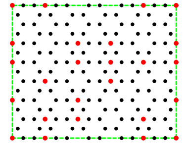
Figure 3: (Color online)Graphene supercell with $N_{x}$=5 and $N_{y}$=7. Black small circles represent carbon atoms. Larger red circles indicate the position of the adatoms. The adatoms are located in hollow positions and in this figure we plot a particular random realization of disorder. In this figure the number of adatoms per carbon atoms is $x$=17/140.

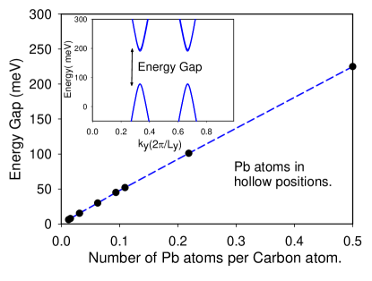
Figure 4: (Color online) In the inset we plot a band structure of a rectangular graphene supercell with $x$=0.25 Pb atoms per carbon. The Pb adatoms induce a gap at the Dirac points ($0,\frac{2\pi}{3L_{x}}$) and ($0,\frac{4\pi}{3L_{x}}$). As commented in the text, the band structure is practically independent of the supercell size and the gap only depends on the concentration of Pb atoms. In the main figure we plot the gap at the Dirac points as function of the Pb atoms concentration. The parameters used in the calculations are taken from reference Calleja et al. (2015).

VI.1 Adatoms in Hollow positions.

In this subsection we analyze supercells with different sizes and forms and with different concentrations of adatoms randomly distributed, but always located in hollow positions. In Fig.3 we show an example of supercell of size $N_{x}$=5, $N_{y}$=7 with 17 adatoms deposited in a random way in hollow positions. In the inset of Fig.4 we plot a typical band structure obtained for an adatom concentration $x$=0.25. The adatoms open a gap at the Dirac points and, in agreement with the results presented in subsection V.1, the band structure corresponds to a Dirac equation in presence of an intrinsic SOC, equations 4 and 6. In our numerical calculations we obtain that for atoms adsorbed in hollow positions, the band structure always has this form, independently of supercell size and form or disorder realization. The SOC depends only on the heavy atoms concentration. In Fig.4 we plot the energy gap as function of the adatom concentration, $x$. The dependence is practically linear and this indicates an almost null interference effect between adatoms.

We understand this linear dependence using Green function techniques. The low energy properties of an electron are described by the Dirac equation $\hbar v_{F}\sigma_{0}\,(sk_{x}\tau_{x}+k_{y}\tau_{y})$ and the corresponding Green function is

$$G_{0}({\bf k},\omega) = \frac{1}{\hbar\omega-H_{0}}$$ (39)

$$= \frac{\sigma_{0}}{\hbar\omega^{2}-\hbar v_{F}^{2}k^{2}}\left(\begin{array}[]{cc}\omega&v_{F}ke^{i\theta_{\bf k}}\\ v_{F}ke^{-i\theta_{\bf k}}&\omega\end{array}\right)$$

Here $\theta_{\bf k}$=$\tan^{-1}\frac{k_{y}}{sk_{x}}$. An adatom located in a hollow position, at ${\bf r}_{i}$, produces a scattering potential of the form, $s\,\sigma_{z}\tau_{z}\delta(\bf r-\bf r_{i})$. In presence of a density, $x$, of adatoms in hollow positions and neglecting multiple scattering, the Green function of the total Hamiltonian isEconomou (2006)

$$G({\bf k},\omega)=G_{0}({\bf k},\omega)+x\Delta s\sigma_{z}G_{0}({\bf k},\omega)\tau_{z}G({\bf k},\omega)\,\,.$$ (40)

Inverting this equation we get,

$$G({\bf k},\omega) = \frac{1}{\hbar^{2}\omega^{2}-\hbar^{2}v_{F}^{2}k^{2}-x^{2}\Delta^{2}}\times$$ (43)

$$\left(\begin{array}[]{cc}\hbar\omega+x\Delta s\sigma_{z}&\hbar v_{F}ke^{i\theta_{\bf k}}\\ \hbar v_{F}ke^{-i\theta_{\bf k}}&\hbar\omega-x\Delta s\sigma_{z}\end{array}\right)$$

that corresponds to the virtual crystal Hamiltonian $H$=$H_{0}$+$x\Delta s\sigma_{z}\tau_{z}$, describibg graphene in presence of an intrinsic SOC of magnitude $x\Delta$.

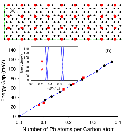
Figure 5: (Color online) (a) Graphene supercell with $L_{x}$=10$\sqrt{3}a$ and $L_{y}$=$5a$. Black small circles correspond to the positions of the carbon atoms. Larger red circles represent adatoms. The adatoms form a rectangular lattice commensurate with the graphene supercell. In the figure the dimensions of the adatom cell are $l_{x}$=$L_{x}/9$ and $l_{y}$=$L_{y}/3$. (b) Inset, band structure for the geometry presented in (a). (b) Main figure, dependence of the energy gap, as defined in the inset, as function of the Pb atoms concentration. Black points are obtained in the graphene supercell fixing the dimension $l_{y}$=$L_{y}/3$ and changing $l_{x}$. Red points are obtained fixing $l_{x}$=$L_{x}/9$ and changing $l_{y}$. The parameters used in the calculation are taken from reference Calleja et al. (2015).

VI.2 Commensurate array of Pb atoms on Graphene.

Graphene grown on Ir(111) forms a 9.3x9.3 moiré superstructure with a $\sim$25Å periodicityN’Diaye et al. (2008). When Pb atoms are intercalated under the graphene monolayer, the Pb atoms form a rectangular lattice commensurate with Ir. Therefore the honeycomb graphene lattice and the array of Pb atoms commensurate in a large moiré supercellCalleja et al. (2015).

In this subsection we study the spin-orbit effects induced by a rectangular array of Pb atoms of dimensions $l_{x}\times l_{y}$ commensurate with a large rectangular graphene supercell of dimensions $L_{x}\times L_{y}$, see Fig.5(a). In the inset of Fig.5(b) we plot, for the geometry shown in Fig.5(a), the electronic states obtained with the tight-binding parameters corresponding to Pb. The band structure coincides with the eigenvalues of the Dirac equation in presence of a Rashba like spin-orbit coupling. The intensity of the SO coupling is proportional to the energy gap between the second conduction band and the second valence band. We find that this gap increases linearly with the Pb concentration,$x$, and only depends on the concentration of Pb atoms being independent of geometrical details. In Fig.5(b) we plot the energy gap as function of $x$ for a graphene supercell characterized by $N_{x}$=10 and $N_{y}$=5, and different combination of $i_{x}$ and $i_{y}$. We obtain the same linear dependence for larger graphene supercells.

These results indicate that Rashba coupling induced from different adatoms do not interfere and the total Rashba coupling is just the sum of the different contributions. The Rashba SO coupling induced by Pb adatoms have always the same sign, dictated by the broken mirror symmetry, and the linear behavior reveals that in the commensurate phase, the adatoms average all possible locations in the graphene unit cell. On the contrary, the absence of a gap at the Dirac points indicates that the contribution to intrinsic SOC from adatoms located in different places sums zero. This occurs because the sign of the intrinsic SOC induced by adatoms depends on its location. A particular example is the case of the intrinsic SOC induced by adatoms in hollow position, Eq.32, that has opposite sign than the induced by adatoms located in top positions Eq.33.

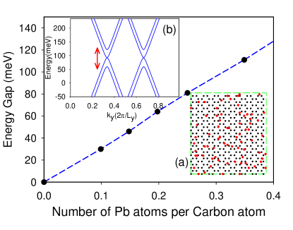
Figure 6: (Color online) (a) Graphene supercell with $L_{x}$=7$\sqrt{3}a$ and $L_{y}$=$13a$. Black small circles correspond to the positions of the carbon atoms. Larger red circles represent adatoms. The concentration of adatoms is $x$=0.2 and they are located in a random way. (b) Inset, band structure for the geometry presented in (a). Main figure, dependence of the energy gap, as defined in the inset, as function of the Pb atoms concentration. The energy gap only depends on Pb concentration and is independent on geometry or disorder realization. The parameters used in the calculation are taken from reference Calleja et al. (2015).

VI.3 Random Positions

Finally we compute the SO induced in graphene by a concentration of Pb adatoms randomly distributed. We study large graphene unit cells, Fig.6(a), with different concentration of adatoms. The main results of the simulations are that there is not band gap at the Dirac points of the band structure, Fig.6(b), and the Rashba like SOC increases linearly with the concentration of Pb atoms, Fig.6. These results are independent on the disorder realization and size and form of the unit cell. The dependence of the SOC on Pb concentration is the same than in the case of commensurate supercell. This, and the absence of intrinsic like SOC indicate that in both cases, commensurate order and random positions, there is not interference effects between adatoms, and the resulting SOC is just the sum of the contributions from adatoms placed in different positions.

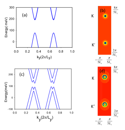
Figure 7: (Color online)(a)Band structure of a graphene supercell ($N_{x}$=5, $N_{y}$=7) with a concentration $x$=0.25 of adatoms randomly located in hollow positions. (b) Partial section of the Brillouin zone showing in green, the regions that contribute to the spin up Hall conductivity $\sigma_{xy}^{\uparrow}$ for the case (a). (c) Same than (a) for a fully random distribution of adatoms and an exchange field of 18$meV$. (d) Partial section of the Brillouin zone showing in green the regions that contribute to the total Hall conductivity $\sigma_{xy}^{\uparrow}$ + $\sigma_{xy}^{\downarrow}$ for the case (c).

VII Topological Properties.

In the previous Sections we have obtained that a graphene layer doped with adatoms placed in hollow positions has a gapped energy band structure similar to that obtained from the Dirac equation with an intrinsic SOC. On the contrary adatoms randomly or commensurately distributed on graphene generate a gapless band structure that remind that of graphene with Rashba SOC. In this Section we check that both adsorption geometries, hollow and random, have the same topological properties that the Dirac equation plus intrinsic and Rashba SOC respectively. In order to know the topological properties, we compute the spin resolved Hall conductivity of the system,

$$\sigma_{xy}^{\sigma}=-2\sum_{n,n^{\prime},{\bf k}}\frac{{\rm Im}\left(<n{\bf k}|v_{x}\hat{P}_{\sigma}|n^{\prime}{\bf k}><n^{\prime}{\bf k}|v_{y}\hat{P}_{\sigma}|n{\bf k}>\right)}{(\varepsilon_{n,{\bf k}}-\varepsilon_{n^{\prime},{\bf k}})^{2}}$$ (44)

where $|n{\bf k}>$ and $\varepsilon_{n{\bf k}}$ are the eigenfunction and eigenvectors respectively of the supercell Hamiltonian Eq.36, in the sum the index $n$ and $n^{\prime}$ run over occupied and empty states respectively, $v_{\nu}$=-$\frac{1}{\hbar}\frac{\partial H}{\partial k_{\sigma}}$ is the velocity operator in the $\nu$-direction and $\hat{P}_{\sigma}$ projects the wave function in the subspace of spin $\sigma$.

In the case of adatoms in hollow positions we have obtained

$$\sigma_{xy}^{\sigma}=\sigma\frac{e^{2}}{h}\,\,\,\,\,\,\,\rm{adatoms\,in\,hollow\,positions.}$$

that corresponds to a quantum spin Hall systemKane and Mele (2005). The total Hall conductivity sums zero, as it should be in a system with time reversal symmetry. The main contributions to the Hall conductivity come from circular regions centered at the Dirac points, Fig.7(a)-(b).

Adatoms placed randomly on graphene do not generate a gap in the band structure, and the Hall conductivity is zero. However, in references Qiao et al. (2010) and Tse et al. (2011), it was proposed that an exchange field applied to graphene in presence of Rashba SOC should open a gap and the system would be a non trivial insulator characterized by an anomalous quantized Hall effect. We have applied an uniform exchange field to the randomly doped graphene and we have obtained a gapped band structure, Fig.7(c) and a finite Hall conductivity,

$$\sigma_{xy}=\sigma_{xy}^{\uparrow}+\sigma_{xy}^{\downarrow}=2\frac{e^{2}}{h}\,\,\,\,\,\,\,\rm{adatoms\,in\,random\,positions.}$$

that proves that adatoms placed randomly on graphene generated a Rashba SOC. In this case, and because the form of the bands Fig.7(c), the main contributions to the Hall conductivity come from annulus centered at the Dirac points, Fig.7(d).

The realization of the quantum spin Hall effect and quantum anomalous Hall effect for hollow and random adatoms respectively , shows the stability of these topological phases even for a non uniform distribution of the adatoms.

VIII Summary.

In this work we have studied the spin orbit coupling induced in graphene by heavy adatoms with active electrons residing in $p$-orbitals. Depending on the location of the adatoms we find different induced SOC’s. Adatoms located in hollow positions open a gap at the Dirac points and induce an intrinsic like SOC. However adatoms randomly placed or commensurate with the graphene lattice maintain the system gapless and induce a Rashba like SOC. The adatoms only perturb the pristine graphene band structure near the Dirac points.

We find that the SOC induced by the adatoms is additive and there is not interference effects or multiple scattering. The topological properties of graphene with hollow or random adatoms are the same than those of the Dirac Hamiltonian in presence of intrinsic or Rashba SOC respectively. The finite value of the Hall conductivity of graphene doped in different geometries indicates the robustness of the topological phases against a non uniform distribution of the spin orbit coupling.