Slowly increasing elongations of non-spherical asteroids caused by collisions

Abstract

Asteroids are frequently colliding with small projectiles. Although each individual small collision is not very important, their cumulative effect can substantially change topography and also the overall shape of an asteroid. We run simulations of random collisions onto a single target asteroid represented by triaxial ellipsoid. We investigated asteroids of several hundred meters to about $18\,{\rm km}$ in diameter for which we assumed all material excavated by the collision to escape the asteroid. The cumulative effect of these collisions is an increasing elongation of the asteroid figure. However, the estimated timescale of this process is much longer than the collisional lifetime of asteroids. Therefore, we conclude that small collisions are probably not responsible for the overall shape of small asteroids.

1 Introduction

Collisions between asteroids are a very important process, which affects their spins (Harris & Burns 1979, Harris 1979), size distribution (Dohnanyi 1969, Cellino et al. 1991) and also their shapes (Catullo et al. 1984, Farinella & Zappalà 1997, Tanga et al. 2009). Subcatastrophic collisions, however, are not very well described yet and in evolutionary models of asteroid populations, they are only roughly approximated.

The role of small collisions on the overall shape of asteroids was studied in two-dimensional model of Ronca & Furlong (1979). They used similar assumptions in the construction of their model as we do and for the initially elliptical asteroid model they obtained increasing elongation of its shape. Later, Harris (1990) mentioned this effect when discussing collisional evolution of the spin of nonspherical asteroids.

Numerical investigation of asteroid shape evolution by collisions was presented by Korycansky & Asphaug (2001) and Korycansky & Asphaug (2003) (hereafter KA03). Their model is based on excavation, orbit and reimpact of the ejecta from the cratering event and also on the conservation of the maximum angle of repose of the material on the surface of the model asteroid. KA03 conclude that the final shape is mostly oblate ellipsoid indepedently of the initial conditions. They also calculated the timescale of such impact-induced reshaping of the asteroid to be more than an order of magnitude longer than catastrophic disruption timescale.

Szabó & Kiss (2008) report about shape distribution of asteroid families derived from multi-epoch photometry of the Sloan Digital Sky Survey Moving Object Catalog. They conclude that younger families seem to contain more elongated asteroids, while older families contain more rounded asteroids. In their opinion, this is in agreement with the predictions of an impact-driven evolution of the asteroid shapes (KA03). Domokos et al. (2009) studied the role of micro-collisions on the overall shape of asteroids in their averaged continuum abrasion model. Their asteroid models evolve to prolonged shapes that possess large, flat areas separated by edges.

In the present paper we want to discuss the effect of a large number of subcatastrophic collisions on the shape of an asteroid. This problem caught our interest when constructing an evolutionary model of asteroid rotations influenced by subcatastrophic collisions focused on tumbling asteroids (Pravec et al. 2005). We noticed that our model asteroids subjected to collisions became ever more elongated than at the beginning of the simulation. Since we wanted to ensure it was not just a numerical issue of our model, we started to investigate this effect.

We give a detailed description of our model and the method used in Section 2. Section 3 contains an estimate of timescale of the increasing elongation process. Numerical results are given in Section 4. In Section 5, we discuss some implications and caveats of the present research and conclusions are given in Section 6.

2 Increasing elongation of the model asteroid

An obvious effect of a small collision is a formation of impact crater on the surface of an asteroid. There is, however, a cumulative effect of a large number of such cratering events as well. In our analytical model of subcatastrophic collisions between a target asteroid and a large number of small projectiles, we noticed that the shape of an initially elongated asteroid becomes gradually more elongated. More exactly, it was changing the shape of a dynamically equivalent equal-mass ellipsoid. Its semiaxes are defined as (Kaasalainen 2001, Pravec et al. 2014)

$$a_{\rm dyn}^{2}=\frac{I_{b}-I_{a}+1}{I_{a}+I_{b}-1}\qquad b_{\rm dyn}^{2}=\frac{I_{a}-I_{b}+1}{I_{a}+I_{b}-1}\qquad c_{\rm dyn}=1\,,$$

and

$$I_{a}=I_{1}/I_{3}\qquad I_{b}=I_{2}/I_{3}\,,$$ (1)

where $I_{1}$, $I_{2}$ and $I_{3}$ are the principal moments of inertia of the target asteroid and $I_{a}$ and $I_{b}$ are normalized principal moments of inertia of the dynamically equivalent ellipsoid; $I_{c}=1$.

In our model, the target asteroid was represented by a triaxial homogeneous ellipsoid. We ran a series of consecutive collisions with the target, each forming an impact crater on the surface of the ellipsoid according to the scaling laws of Holsapple (1993) and Holsapple & Housen (2007), with the angular momentum transfer efficiency based on laboratory experiments of Yanagisawa et al. (1996) and Yanagisawa & Hasegawa (2000) and updating the inertia tensor of the target asteroid after every single collision.

The impact speed was $5\,{\rm km\,s^{-1}}$, which is the median impact speed in the central regions of the Main Asteroid Belt (Bottke et al. 2005). The geometry of collisions was isotropic with respect to the target surface (the probability of a collision from any direction was the same) with one exception: We only allowed collisions for which incidence angle (the angle between the impact velocity vector and the normal to the surface at the impact site) was less than 75 degrees. We simply wanted to avoid almost tangent impact geometries, since the formation of impact craters for such impact geometries is not very well understood yet.

The target was in a principal axis rotation state before the collision. Initial rotation period was chosen randomly according to the observed distribution of rotation periods of small Main Belt/Mars Crossing asteroids (Pravec et al. 2008, updated on 2014-04-20). Size of the projectile was random according to a power-law distribution (Bottke et al. 2005).

After every collision, rotation state and shape of the target asteroid changed. However, in this paper we only focus on a change of the shape and we quantify this change as follows. The collision formed an impact crater on the surface of the ellipsoid. We therefore calculated an inertia tensor of the mass that fills the crater and subtracted it from the inertia tensor of the ellipsoid. Then, we updated lengths of axes of the ellipsoid using the values of the dynamically equivalent ellipsoid. We also reset the shape of the target asteroid to the triaxial ellipsoid (erased the impact crater) keeping its density on the initial value (which lead to decreasing size of the target asteroid).

In our simulations, we only investigated the effect of subcatastrophic collisions. This corresponds to the calm period of an asteroid’s life between larger shattering or even dispersal events (shattering causes large scale damage to the asteroid, but most of its pieces remain gravitationally bound; dispersal event reduces the target to one-half its original mass, Melosh & Ryan 1997, Housen 2009). We used two criteria to recognize a subcatastrophic collision. First, we compared the specific energy of the collision with the shattering criterion. In our calculations, we followed Stewart & Leinhardt (2012), who derived the dispersal criterion in gravity regime of collisions in their numerical simulations. We calculated the shattering criterion as 1/4 of their value according to Housen (2009). Second, we calculated the maximum size of an impact crater for a given size of the target asteroid according to the relation of Burchell & Leliwa-Kopystyński (2010). The collision was subcatastrophic if both these conditions were met.

There is a set of mechanical properties of the target and the projectile, which can be varied in a physically plausible range. We did this to some extent in our previous paper, Henych & Pravec (2013), and we found that these values affect the size of an impact crater formed on the surface of the target asteroid. Therefore, they affect the timescale of increasing elongation of the target’s shape. In the present research, we have chosen some plausible values of those parameters and held it constant throughout our simulations as specified in Table 1. The density of the target and of projectiles was the same, $2\,{\rm g\,cm^{-3}}$.

Table 1: Scaling and material constants for non-porous target. $K_{1}$ and $K_{2}$ are experiment-based coefficients, $\mu$ and $\nu$ are the scaling parameters, $\bar{Y}$ is a material strength and $K_{r}$ and $K_{d}$ are the shape constants, cf. Holsapple (2003).

$K_{1}$	$K_{2}$	$\mu$	$\nu$	$\bar{Y}\,(\rm{MPa})$	$K_{r}$	$K_{d}$
0.095	0.257	0.55	0.33	1	1.1	0.6

Since we are mostly interested in the small asteroid population (bodies of several kilometers in diameter), we ran our simulations for asteroids of mean diameters $0.6$–$17.6\,{\rm km}$ (see Table 2). The upper limit was determined by the fact that almost all material excavated by the hypervelocity impact of a projectile is ejected from the asteroid for asteroid diameters of less than about $18$–$20\,{\rm km}$ according to scaling laws (Housen & Holsapple 2011). This was calculated by using the scaling laws for ejecta speeds as described by Housen & Holsapple (2011) and comparing it with the surface escape speed.

The mean diameter of the target is

$$D_{\rm t}=2(abc)^{1/3}\,,$$ (2)

where $a$, $b$ and $c$ ($a\geq b\geq c$) are the semiaxes of the triaxial ellipsoid representing the target asteroid. In our simulations, we concentrated on two effects – the shape and the size dependence of the collisional erosion. Therefore, we ran longer series of $1{,}000$ collisions for various target asteroid sizes (see Table 2) and fixed initial axial ratios of $a/c=2.0$ and $b/c=1.4$. For each target size we ran three separate runs to exclude any numerical artifacts. Then, we ran shorter series of about $110$ consecutive collisions, where we fixed $c=0.5\,{\rm km}$ and varied the initial semiaxes ratios (see Table 3).

Table 2: Effective diameters of model asteroids in long series of collisions and limiting projectile sizes. The fixed initial semiaxes ratios of the target were $a/c=2.0$ and $b/c=1.4$, $D_{\rm t}$ is the target mean diameter, $D_{\rm p,max}$ is the largest projectile, $D_{\rm p,min}$ is the smallest one.

$c~{}[\rm{km}]$	0.2	0.35	0.5	1.5	2.5	4.25	6.25
$D_{\rm t}~{}[\rm{km}]$	0.6	1.0	1.4	4.2	7.0	12.0	17.6
$D_{\rm p,max}~{}[\rm{m}]$	5.5	10.5	16.0	78.0	150.0	291.0	437.0
$D_{\rm p,min}~{}[\rm{m}]$	1.0	1.0	1.0	1.0	1.0	1.0	1.0

Table 3: Semiaxes ratios of the ellipsoid representing the target asteroid used in our simulations (semiaxes $a$, $b$, $c$). The shortest axis was $c=0.5\,{\rm km}$.

$a/c$	1.1	1.2	1.3	1.3	1.30	1.4	1.4	1.4	1.5	2.0
$b/c$	1.1	1.2	1.3	1.2	1.14	1.4	1.1	1.2	1.2	1.4

3 Timescale estimates

The importance of erosional process for evolution of asteroid shapes is determined by the timescale of this process. We calculated the timescale in two different ways and obtained very different results. We also have the timescale indicated by the numerical simulations as explained in a following subsection. We discuss the differences between the two timescale calculations at the end of this section after their description.

3.1 Timescale of the erosion from the simulations

The timescale of the increasing elongation of the asteroid figure can be estimated directly from the simulations. We filtered size of the projectiles for a specific size of the target to keep the collisions subcatastrophic (see Table 2). However, we also saved information about discarded projectiles, whether too small or too large. Therefore, we have the relative timescale of the increasing elongation in comparison to the catastrophic disruption of the target asteroid caused by projectiles larger than upper size limit.

In all our simulation runs with $1{,}000$ subcatastrophic collisions, the target asteroid was hit be the projectile larger than upper size limit after a few subcatastrophic collisions. Therefore, we estimate the timescale of the process to be at least two orders of magnitude longer than the collisional lifetime of the target asteroid.

3.2 Ejected mass measure

The first and probably more reliable and solid calculation compares the erosional effect of projectiles in terms of excavated and ejected mass. As noted above, practically all mass excavated by the projectile escapes the target asteroid for sizes used in our calculations. The total eroded mass by the population of projectiles can be calculated as

$$M_{\rm er}=\int^{D_{\rm p,max}}_{D_{\rm p,min}}\frac{1}{4}p_{\rm i}(D_{\rm t}+D_{\rm p})^{2}\Delta tAV_{\rm p}n(D_{\rm p}){\,\rm d}{}D_{\rm p}\,,$$ (3)

where $p_{\rm i}$ is the intrinsic probability of collision, $D_{\rm t}$ and $D_{\rm p}$ are the target and the projectile diameters, respectively, $\Delta t$ is the timescale we are looking for, $V_{\rm p}$ is the volume of the projectile, $A$ is a factor describing the excavated material volume, $n(D_{\rm p})$ is the distribution function of the projectile sizes and $D_{\rm p,min}$ and $D_{\rm p,max}$ are the minimum and maximum projectile size, respectively.

We define the timescale of erosion process as a time interval over which half the target initial mass is excavated by subcatastrophic collisions. Then, $M_{\rm er}=0.5M_{\rm t,initial}$ and when we integrate Eqn. 3 we obtain the timescale

$$\Delta t=\frac{12(s+4)M_{\rm t,initial}}{p_{\rm i}\pi ABD^{2}_{\rm t}(D_{\rm p,max\phantom{i}}^{s+4}\!\!-D_{\rm p,min}^{s+4})}\,,$$ (4)

where we used $V_{\rm p}=D^{3}_{\rm p}\pi/6$ for spherical projectiles, $s=-2.574$ is the exponent of the distribution $n(D_{\rm p})=BD_{\rm p}^{s}$, $D_{\rm p}$ is the projectile diameter and we approximated $(D_{\rm t}+D_{\rm p})^{2}\approx D^{2}_{\rm t}$, since the projectile’s diameter is much smaller than the target’s diameter (few percent for the largest projectiles in our simulations). For $s=-2.574$ used in our simulations, the calculation of $\Delta t$ is not very sensitive to specific values of $D_{\rm p,max}$ and $D_{\rm p,min}$, because we measure the erosion efficiency of every projectile that collided with the target asteroid. When we set $D_{\rm p,min}=1\,{\rm mm}$ instead of $1\,{\rm m}$ used in our simulations, the calculated timescale barely changes. The constant $A$ can be derived from the scaling laws or found from the graph of ejected mass vs. projectile diameter of all our simulations (see Fig. 1). The constant $B=5.07\,{\rm km^{-s-1}}$ for the projectile size distribution we used (Bottke et al. 2005). More details on derivation of these relations are in Appendix A.

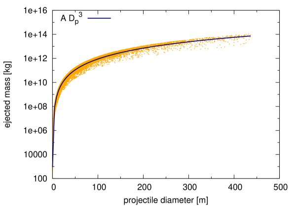
Figure 1: Erosion efficiency of projectiles in all our simulations measured by ejected mass vs. projectile diameter. The ejected mass is proportional to the volume of the projectile. The vertical spread of the points for a specific projectile diameter is caused by various impact geometries.

3.3 Number of collisions measure

The second approach is based on a calculation of the number of collisions with specified population of projectiles for a single target.

We first calculate the collisional lifetime of a model asteroid as (Farinella et al. 1998)

$$t_{\rm shatter}=20\,{\rm Myr}\sqrt{R_{\rm t}}\,,$$ (5)

where $R_{\rm t}$ is the mean target asteroid radius in meters. We note that this collisional lifetime estimate is derived for smaller asteroids and it underestimates lifetime for asteroids in our simulations. The collisional lifetime for asteroids larger than several hundred meters as calculated by Bottke et al. (2005) is more complicated function, but in general it has a steeper slope than that of Farinella et al. (1998).

Then, we calculate a number of subcatastrophic collisions that the asteroid experiences during its collisional lifetime. In our simulations, we introduced a cutoff of the projectile size equal to $1\,{\rm m}$ because of quickly growing calculation expenses with decreasing size of projectiles. We think that smaller projectiles are not very relevant for this effect but more extensive calculations will have to be done to check this in the future.

The number of collisions for a single target is (O’Brien & Greenberg 2005)

$$n_{\rm coll}=p_{\rm i}(R_{\rm t}+R_{\rm p})^{2}N_{\rm p}\Delta t\,,$$ (6)

where $p_{\rm i}$ is the intrinsic probability of collision, $R_{\rm t}$ and $R_{\rm p}$ are the target and the projectile radii, respectively, $N_{\rm p}$ is the number of projectiles in this region and $\Delta t$ is the time interval for which we calculate the number of collisions. We take this equal to the $t_{\rm shatter}$ as calculated by Eqn. 5. We assume the model asteroid is a member of the Main Asteroid Belt. The intrinsic probability is taken from Cibulková et al. (2014) as $p_{\rm i}=4.91\times 10^{-18}\,{\rm km^{-2}yr^{-1}}$.

The number of projectiles is calculated assuming that the distribution of asteroid sizes in the Main Asteroid Belt is a power law as already mentioned above (Bottke et al. 2005). The number of bodies in the size interval from $D_{\rm p,min}$ to $D_{\rm p,max}$ is

$$N(D_{\rm p,min},D_{\rm p,max})=\frac{10^{q}}{s+1}(D_{\rm p,max}^{s+1}-D_{\rm p,min}^{s+1})\,,$$ (7)

where we use the same size distribution as in Eqns. 3 and 4 and $q={\rm log}_{10}B$. The projectile sizes used for various target sizes are in Table 2. The upper limit is given by disruption criterion (Stewart & Leinhardt 2012 and Housen 2009) and the lower limit is chosen somewhat arbitrarily to keep the computational expenses reasonable. Finally, a rough estimate of a timescale of the increasing elongation can be calculated. It is

$$t_{\rm reshape}=\frac{t_{\rm shatter}}{n_{\rm coll}}\frac{\delta_{\rm reshape}}{\delta_{\rm avg}}\,,$$ (8)

where $\delta_{\rm reshape}$ is the magnitude of a relative change of any semiaxis of the asteroid after that the asteroid will experience some abrupt change of shape and $\delta_{\rm avg}$ is the average relative change of the same ratio per one collision. We discuss the former value in the next paragraph, the latter value comes from our simulations. Also note, that this timescale actually does not depend on the asteroid lifetime (put the Eqn. 6 to the Eqn. 8).

According to Harris et al. (2009), there are no photometric observations of asteroids implying bodily axial ratio higher than about $3$. Therefore, we chose the value of $\delta_{\rm reshape}=3/2$ for the most elongated initial asteroid model used in our simulations (initial axial ratios $2\!:\!1.4\!:\!1$) and $\delta_{\rm reshape}\simeq 2.7$ for an almost spherical initial asteroid model (initial axial ratios $1.1\!:\!1.1\!:\!1$).

3.4 Comparison of the two measures

We decided to prefer the timescale measure based on the ejected mass which is a kind of efficiency measure for every projectile. This measure gives more realistic timescale estimate and is also consistent with the relative timescale of the process based on our simulations.

When we analyzed our simulations we concluded that substantial change of the axial ratio was only caused by the very largest projectiles (or the collisions close to the shattering threshold). Even though smaller projectiles are more populous thanks to the power-law distribution of their sizes (the exponent being lower than $-2$), their cumulative effect does not balance the effect of the largest projectiles. It is necessary to somehow weight the excavation efficiency of the projectiles otherwise the $n_{\rm coll}$ is overestimated and $t_{\rm shatter}$ is consequently underestimated. Therefore the timescale measure based solely on the number of all collisions is unrealistically skewed to the small values.

4 Results

In our simulations, we observed that the elongation of the target asteroid gradually increases with increasing number of collisions. As described in Section 2, we did not calculate a change of the actual shape of the target but rather a change of the shape of a dynamically equivalent equal mass ellipsoid. We calculated its semiaxes from the inertia tensor of the target asteroid gradually changed by consecutive collisions forming craters and hence removing material from the asteroid.

An example of three series of collisions onto the target asteroid with initial semiaxes ratios of $a/c=2.0$ and $b/c=1.4$ and mean diameters of $4.2$ and $17.6\,{\rm km}$, respectively, is shown in Fig. 2. The graph shows the evolution of $a/c$, and $b/c$ axial ratios vs. cumulative projectile mass divided by the initial target mass on the lower abscissa and cumulative excavated mass divided by the initial target mass on the upper abscissa. It can be seen that the two ratios tend to increase as more projectiles impact the target. Other simulations look similar to this example.

In Fig. 2, we also plot three series of collisions for a model of a “weak 17.6-km” asteroid for which we set the same shattering threshold $Q^{*}_{\rm S}$ as for the 4.2-km asteroid. We ran these series to evaluate our hypothesis that the apparently faster erosion of the larger asteroid models is an artifact caused by their higher shattering thresholds as will be discussed in Sect. 5. The black dots in the graph depict the analytical model of Harris (1990) which represents the erosion by removal of the constant-depth layer from the ellipsoidal asteroid model. This model is size-independent (contrary to our model) and its apparent consistency with collisional erosion of our 17.6-km asteroid model is largely coincidental.

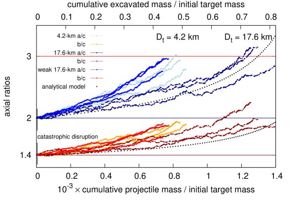
Figure 2: Series of successive collisions onto two asteroids of various mean diameters represented by ellipsoids with initial $a/c=2.0$ and $b/c=1.4$. The lower abscissa is cumulative projectile mass divided by the initial target mass, the upper abscissa is cumulative excavated mass divided by the initial target mass. Changing axial ratios are in the ordinate. We also plot the simple analytical model of Harris (1990) (black dots), the “weak 17.6-km” asteroid model with the same shattering threshold as the 4.2-km asteroid model and we mark the collisional lifetime of the model asteroids. See text for details.

In the following Fig. 3, there are results of the timescale calculation of the erosional process for various size of the target asteroid. It shows both, the time needed to erode half the initial target mass by subcatastrophic collisions off the asteroid (Sect. 3.2) and also the time of reshaping the target asteroid from the initial axial ratio $a/c=2.0$ to the axial ratio $a/c=3.0$ (Sect. 3.3). The timescale is in millions of years. It is obvious from Fig. 3 that both timescales are much longer than collisional lifetime for most asteroids in our simulations.

The displayed timescales calculated by two different methods are similar for smaller asteroids but they diverge for larger asteroids. As already discussed in Sect. 3.4., we prefer the timescale calculation based on the ejected mass (orange circles in Fig. 3) and all our conclusions come from this calculation.

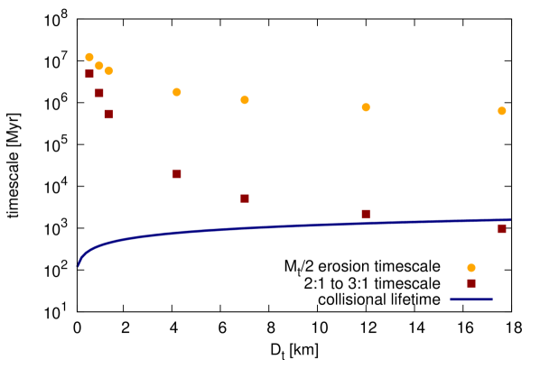
Figure 3: The timescale of the collisional erosion calculated in two ways. Orange circles are calculated as the time after which half the initial asteroid mass is ejected by collisions, dark-red squares are calculated using the number of small collisions experienced by the target asteroid during its collisional lifetime. The collisional lifetime is calculated by Eqn. 5 (Farinella et al. 1998).

The initial elongation of the asteroid (shorter series of collisions) leads to faster erosion. The timescale calculation is affected by larger mean diameter of an asteroid $D_{\rm t}$ in Eqn. 4 and also by wider interval of projectile sizes for more elongated asteroids.

5 Discussion

The explanation for the results of our simulations can be found in Harris (1990). Cratering erosion tends to change all dimensions by the same amount on average. Imagine a triaxial ellipsoid subjected to isotropic random impacts. We will concentrate only on the changing dimensions of the longest and the shortest axes of the ellipsoid for a while. We observe that impacts erode relatively larger part of the shortest axis of the ellipsoid than its longest axis. This leads to the increasing elongation of the ellipsoid or the ratio of the longest to the shortest axes leghts. That is exactly what we see in our present simulations as shown in Fig. 2.

However, from the results it is obvious that the timescale of this process is several orders of magnitude longer than the collisional lifetime of the asteroid. It is also visible in Fig. 3 that for increasing size of the target asteroid the erosion is faster. It is probably caused by the increasing specific energy threshold in gravity regime for the asteroid sizes from about $0.6\,{\rm km}$ used in our simulations (see, e.g., a review by Holsapple et al. 2002 and their Fig. 6). It means that larger asteroid can sustain larger collisions which excavate more material. In Fig 2, it can be seen that the “weak 17.6-km” asteroid model behaves much like the 4.2-km asteroid because it cannot sustain larger craters than this smaller asteroid. Therefore, we think that this strengthening (by gravity) of asteroids with increasing size is responsible for faster collisional erosion.

This is also supported by direct observations of large impact craters on various small solar system bodies. We illustrate this in Fig. 4 which we compiled from crater sizes and the parent bodies sizes listed in Thomas (1999), Asphaug (2008) and Burchell & Leliwa-Kopystyński (2010). The graph shows that larger bodies bear relatively larger impact craters.

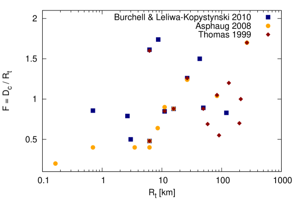
Figure 4: Relative sizes of large craters observed on small solar system bodies vs. mean body radius. Relative size $F$ is a ratio of the crater diameter and the mean body radius. Larger bodies usually bear relatively larger impact craters. Overlapping points are the same craters on the same objects.

We came to the similar conclusion as KA03, however, our particular results differ substantially. Our models are quite different and we think it could be useful to combine their main features to study the role of small collisions in a more complex way.

In our model, we did not work with the actual shape of the asteroid but with the dynamically equivalent ellipsoid as described above. Probably more serious drawback of our model is the absence of “landsliding” that was present in KA03 and is probably important for a shape relaxation to equilibrium (there is a limit of the angle of repose of the surface material observed on the asteroids studied by spacecraft mission as well as predicted by theory).

On the other hand, our model deals with angular momentum evolution of the target asteroid caused by projectiles, mass loss caused by impact excavation and we also allow for large craters up to the shattering threshold. All these characteristics were mentioned by KA03 as future plans of the modelling of impact evolution of shapes of asteroids.

Important difference between our and KA03’s model is that we do not model ejecta’s orbits and their reimpact on the surface of the target asteroid. In our model, all ejected material escapes the asteroid. This makes the model only valid for small asteroids in the size range of several hundred meters to about $18$–$20\,{\rm km}$ (see Sect. 2 for details).

We also differ in the resulting shape of the asteroids subjected to a series of small collisions. While KA03 obtained oblate shape in most of their simulations, we predict the elongation will grow for an already elongated initial shape. Our result seems to be consistent with an expected behaviour of large number of collisions as noted above. KA03 also noted the dependence of the result on the initial spin rate. We cannot verify this result since our model asteroids had random rotation period as described in Sect. 2.

We predict even longer timescale of the erosion than KA03 which can be attributed to different construction of the model and the timescale calculation. However, the qualitative result is the same – the timescale is several orders of magnitude longer than the collisional lifetime of the asteroid for the projectile population exponent $s=-2.574$.

What follows are few caveats concerning the construction of our model. It has several points that are affected by large uncertainties. First, scaling laws for impact crater formation were developed for halfspace impacts, not for impacts onto curved surfaces and also we used earth rock material constants which may or may not be realistic.

Second, the catastrophic disruption threshold comes from numerical simulations and scaling and is only one of many that can be found in literature as there is quite a large uncertainty in this.

Third, there is a large uncertainty in population estimates of such small projectiles (and also targets), since we are well beyond present observation size limit. The power-law exponent is taken from the numerical model of the Main Asteroid Belt evolution of Bottke et al. (2005). Other values are possible and would lead to faster or slower evolution of the asteroid shape.

Fourth, there is quite a questionable assumption about the isotropic distribution of projectiles. We assumed that the Main Belt asteroids have some moderate range in orbit inclination and also that the rotation axes of the target asteroids are randomly oriented. This last assumption may be erroneous, though, because small Main Belt asteroids may be trapped in Slivan state (Vokrouhlický et al. 2003) caused by the Yarkovsky–O’Keefe–Radzievskii–Paddack (YORP) effect which makes obliquity of their rotation axis gain specific values. It is, however, not clear whether this mechanism also works for smaller, km-sized asteroids. The above mentioned paper indicates that asteroids smaller than about $10\,{\rm km}$ may be able to leave the resonant spin state.

6 Conclusions

In a present paper we describe the effect of increasing elongation of a model asteroid represented by a homogeneous triaxial ellipsoid caused by consecutive small collisions. The changing shape of our model asteroid was indicated by changing intertia tensor and axial ratios of a dynamically equivalent equal mass ellipsoid. The effect can be explained by the fact that the shorter axis of the ellipsoid decreases relatively faster than the longer one for large number of isotropically distributed collisions.

However, the estimated timescale of this process seems to be much longer than collisional lifetime of asteroids in the size range of several hundred meters to about $20\,{\rm km}$. Therefore, this effect is probably not very important in formation of overall asteroid shapes and their evolution, unless some of our assumptions is unrealistic. For instance, if the exponent of the power-law projectile size distribution was smaller than $s=-2.574$, the erosion would be faster. It is therefore important to set new observational constraints on the small projectile population so that we can obtain more accurate timescale estimates.

There is a group of newly discovered asteroids called Barbarians after its first member, 234 Barbara, that are thought to be very old according to their polarimetric and spectral properties (Tanga et al. 2015). These observations indicate rather high content of calcium-aluminium-rich inclusions (Sunshine et al. 2008). Collisional erosion may possibly play some role for larger long living asteroids, but our present model cannot deal with reacumulated ejecta effects, that are necessary to include for asteroids larger than about $20\,{\rm km}$ in diameter. Further investigation of this area is necessary.

Appendix A Ejected mass timescale derivation

Here we derive the relations for erosion timescale estimate based on the excavated mass efficiency of projectiles from the Sect. 3.2. Eroded mass is given by the collision probability of a target asteroid with a diameter $D_{\rm t}$ and a projectile with a diameter $D_{\rm p}$, an efficiency of mass excavation by the projectile given by its volume $V_{\rm p}$ and a proportionality constant $A$ (it is given by the scaling laws of Holsapple 2003) per infinitesimal time interval ${\,\rm d}{}t$ times projectile size distribution $n(D_{\rm p})$. The probability of collision is given by the cross-sectional area of the sum of $D_{\rm t}$ and $D_{\rm p}$ times the intrinsic probability of collision $p_{\rm i}$ (basically the flux of projectiles per area per time, see O’Brien & Greenberg 2005)

$${\,\rm d}{}M_{\rm er}=\frac{1}{4}p_{\rm i}(D_{\rm t}+D_{\rm p})^{2}AV_{\rm p}n(D_{\rm p}){\,\rm d}{}D_{\rm p}{\,\rm d}{}t\,.$$ (9)

We plugin the projectile size distribution $n(D_{\rm p})=BD^{s}_{\rm p}$ (we used that from Bottke et al. 2005), a spherical projectile volume $V_{\rm p}=D^{3}_{\rm p}\pi/6$ and we integrate over a time interval $\Delta t$, projectile size interval from $D_{\rm p,min}$ to $D_{\rm p,max}$ on the right-hand side of Eqn. 9. We also approximate $(D_{\rm t}+D_{\rm p})^{2}\approx D^{2}_{\rm t}$ as the projectile’s diameter is much smaller than target’s diameter (few percent for the largest projectiles in our simulations). We can arbitrarily choose the interval of integration of the left-hand side of Eqn. 9. The reasonable choice is to put $\int\!\!{\,\rm d}{}M_{\rm er}=0.5M_{\rm t,initial}$ because a catastrophic disruption of an asteroid is defined the same way.

When we integrate Eqn. 9, we can finally evaluate the time $\Delta t$ after which the target asteroid subjected to consecutive collisions with a population of projectiles looses half its original mass as

$$\Delta t=\frac{12(s+4)M_{\rm t,initial}}{p_{\rm i}\pi ABD^{2}_{\rm t}(D_{\rm p,max\phantom{i}}^{s+4}\!\!-D_{\rm p,min}^{s+4})}\,.$$ (10)

When we plugin $M_{\rm t,initial}\sim D_{\rm t}^{3}$ to Eqn. 10, we see, that the timescale is proportional to the target’s mean diameter $D_{\rm t}$, inversely proportional to $p_{\rm i}$ (smaller flux of projectiles leads to a longer timescale) and inversely proportional to $A$, or erosion efficiency of projectiles.

References

- Asphaug (2008) Asphaug E., 2008, Meteoritics and Planetary Science, 43, 1075
- Bottke et al. (2005) Bottke W. F., Durda D. D., Nesvorný D., Jedicke R., Morbidelli A., Vokrouhlický D., Levison H. F., 2005, Icarus, 179, 63
- Burchell & Leliwa-Kopystyński (2010) Burchell M. J., Leliwa-Kopystyński J., 2010, Icarus, 210, 707
- Catullo et al. (1984) Catullo V., Zappala V., Farinella P., Paolicchi P., 1984, A&A, 138, 464
- Cellino et al. (1991) Cellino A., Zappala V., Farinella P., 1991, MNRAS, 253, 561
- Cibulková et al. (2014) Cibulková H., Brož M., Benavidez P. G., 2014, Icarus, 241, 358
- Dohnanyi (1969) Dohnanyi J. S., 1969, J. Geophys. Res., 74, 2531
- Domokos et al. (2009) Domokos G., Sipos A. Á., Szabó G. M., Várkonyi P. L., 2009, ApJ, 699, L13
- Farinella et al. (1998) Farinella P., Vokrouhlický D., Hartmann W. K., 1998, Icarus, 132, 378
- Farinella & Zappalà (1997) Farinella P., Zappalà V., 1997, Advances in Space Research, 19, 181
- Harris (1979) Harris A. W., 1979, Icarus, 40, 145
- Harris (1990) Harris A. W., 1990, Icarus, 83, 183
- Harris & Burns (1979) Harris A. W., Burns J. A., 1979, Icarus, 40, 115
- Harris et al. (2009) Harris A. W., Fahnestock E. G., Pravec P., 2009, Icarus, 199, 310
- Henych & Pravec (2013) Henych T., Pravec P., 2013, MNRAS, 432, 1623
- Holsapple et al. (2002) Holsapple K., Giblin I., Housen K., Nakamura A., Ryan E., 2002, Asteroids III, pp 443–462
- Holsapple (1993) Holsapple K. A., 1993, Annual Review of Earth and Planetary Sciences, 21, 333
-
Holsapple (2003)
Holsapple K. A., 2003, Theory and equations for ’Craters from Impacts and
Explosions’, Available online:
http://keith.aa.washington.edu/craterdata/scaling/
theory.pdf, cited on 15 April 2013. - Holsapple & Housen (2007) Holsapple K. A., Housen K. R., 2007, Icarus, 187, 345
- Housen (2009) Housen K., 2009, Planet. Space Sci., 57, 142
- Housen & Holsapple (2011) Housen K. R., Holsapple K. A., 2011, Icarus, 211, 856
- Kaasalainen (2001) Kaasalainen M., 2001, A&A, 376, 302
- Korycansky & Asphaug (2001) Korycansky D. G., Asphaug E., 2001, in Lunar and Planetary Science Conference Vol. 32 of Lunar and Planetary Science Conference, Shaping Asteroids via Small Impacts. p. 1433
- Korycansky & Asphaug (2003) Korycansky D. G., Asphaug E., 2003, Icarus, 163, 374
- Melosh & Ryan (1997) Melosh H. J., Ryan E. V., 1997, Icarus, 129, 562
- O’Brien & Greenberg (2005) O’Brien D. P., Greenberg R., 2005, Icarus, 178, 179
- Pravec et al. (2005) Pravec P., et al., 2005, Icarus, 173, 108
- Pravec et al. (2008) Pravec P., et al., 2008, Icarus, 197, 497
- Pravec et al. (2014) Pravec P., et al., 2014, Icarus, 233, 48
- Ronca & Furlong (1979) Ronca L. B., Furlong R. B., 1979, Moon and Planets, 21, 409
- Stewart & Leinhardt (2012) Stewart S. T., Leinhardt Z. M., 2012, ApJ, 751, 32
- Sunshine et al. (2008) Sunshine J. M., Connolly H. C., McCoy T. J., Bus S. J., La Croix L. M., 2008, Science, 320, 514
- Szabó & Kiss (2008) Szabó G. M., Kiss L. L., 2008, Icarus, 196, 135
- Tanga et al. (2009) Tanga P., Comito C., Paolicchi P., Hestroffer D., Cellino A., Dell’Oro A., Richardson D. C., Walsh K. J., Delbo M., 2009, ApJ, 706, L197
- Tanga et al. (2015) Tanga P., et al., 2015, MNRAS, 448, 3382
- Thomas (1999) Thomas P. C., 1999, Icarus, 142, 89
- Vokrouhlický et al. (2003) Vokrouhlický D., Nesvorný D., Bottke W. F., 2003, Nature, 425, 147
- Yanagisawa & Hasegawa (2000) Yanagisawa M., Hasegawa S., 2000, Icarus, 146, 270
- Yanagisawa et al. (1996) Yanagisawa M., Hasegawa S., Shirogane N., 1996, Icarus, 123, 192