Massive MIMO versus Small-Cell Systems: Spectral and Energy Efficiency Comparison

Abstract

In this paper, we study the downlink performance of two important 5G network architectures, i.e. massive multiple-input multiple-output (M-MIMO) and small-cell densification. We propose a comparative modeling for the two systems, where the user and antenna/base station (BS) locations are distributed according to Poisson point processes (PPPs). We then leverage both the stochastic geometry results and large-system analytical tool to study the SIR distribution and the average Shannon and outage rates of each network. By comparing these results, we observe that for user-average spectral efficiency, small-cell densification is favorable in crowded areas with moderate to high user density and massive MIMO with low user density. However, small-cell systems outperform M-MIMO in all cases when the performance metric is the energy efficiency. The results of this paper are useful for the optimal design of practical 5G networks.

I Introduction

The fifth generation (5G) communications system needs to deliver improvement over 4G, e.g. much higher user data rate/spectral efficiency, enhanced eco-friendliness and energy efficiency, seamless communications, and low latency etc. [1]. To meet the required performance, densified topologies with two main approaches, i.e., massive multiple-input multiple-output (M-MIMO) and small-cell densification, are promising candidate technologies [2].

In M-MIMO, each base station (BS) employs a large-scale antenna array in linear, cylindrical, or other shapes. The large number of antennas not only provides more diversity to the transmission but also “hardens” the channel, allowing low-complexity but sharp beamforming towards the user equipments (UEs) [3]. The results are less interference and higher spectral and energy efficiencies. The main drawback of M-MIMO is the channel estimation/acquisition and feedback, which require a high accuracy to attain the gain that M-MIMO promises [4, 5, 6]. Pilot contamination, itself an existing problem, also restricts the benefits of M-MIMO [4, 7].

In contrast, small-cell networks consists of many micro/femto cells with limited number of antennas, typically one or two, at each access point (AP). Due to the short distance between the APs and UEs, small-cell networks have smaller path loss and co-channel interferences while requiring lower power consumption, hence improving both spectral and energy efficiencies. The gain of small-cell densification, however, is subject to more complicated cell planning and inter-cell coordination/cooperation [8].

The evolution of high spectral/energy efficiency for 5G thus results in two opposing ideas: concentrating the antennas to form M-MIMO BSs, and distributing them to form small cells. It is thus natural to ask which approach performs better and under which scenarios. Despite many works studying either M-MIMO or small-cell networks, there exists few work in literature comparing their performance. One of the reasons is due to system modeling: no existing framework so far allows for an effective collation. In this paper, we aim to partially answer the above question using the metrics of spectral and energy efficiencies. In particular, we resort to stochastic geometry and random matrix theory (RMT) for the analysis. A brief introduction of stochastic geometry can also be found in [9].

RMT, also referred as large-system analysis in literature, was used to investigate large multi-user linear receivers and code division multiple access (CDMA) networks [10, 11] and various MIMO setups [12, 13]. While exact analyses are realizable under finite-dimensional matrix theory [14], they often lead to complicated expressions hence do not provide useful insights. The seminal monograph [15] and other works have shown that large-system analysis can reveal many more interesting properties of communication systems. Furthermore, although the analysis is mathematically accurate only for large random vectors/matrices, the obtained results remain good approximations for finite-dimensional cases. Recently, many studies have also advanced the so-called “deterministic equivalent” approach to investigate more sophisticated system models [16].

M-MIMO, which employs a large number of transmit/receive antennas, is a natural application of large-system analysis. A detailed survey can be found in [17], which lists many key M-MIMO performance analyses considering hardware impairments [18], channel state information (CSI) estimation/acquisition [7, 5], and resource allocation/precoding schemes [19, 20]. Note that most of the M-MIMO studies only consider a BS-centric analysis in which the relative locations of the BSs and UEs are fixed, thus neglecting the network topology. In order to compare M-MIMO with small-cell densification, a proper system modeling is necessary.

In this paper, we study both small-cell and M-MIMO networks using stochastic geometry and large-system tools. The aim is to provide an insightful comparison between these two topologies. The contributions of our paper are summarized as follows:

• System Modeling: We propose a model for M-MIMO and small-cell networks which incorporates the randomness of both transmitting distributed antennas (DAs)/BSs and single-antenna UEs. Particularly, the DA/BS and UE locations are distributed according to Poisson point process (PPPs) with possibly different densities. Therefore, there exists a transmission probability that some transmitting antennas/BSs are turned off due to no associated UE. We assume a time/frequency division multiplexing access (TDMA/FDMA) scheme in which the transmitting nodes associated with more than one UE will communicate with only one UE in each resource block. Finally, we assume non-coordinated DAs/BSs and employ conjugate beamforming, which is optimal for non-coordinated M-MIMO with single-antenna UEs.

• M-MIMO and Small-Cell Network Analysis: We study the performance of M-MIMO and show that the signal-to-interference ratio (SIR) distribution at a typical UE is similar to that under a non-fading ad-hoc network. Here, the important differences between the two cases are the M-MIMO gain and transmission probability. As discussed before, the results for fading ad hoc networks can be directly extended to the small-cell counterparts, with small but important modification again due to the transmission probability. We therefore utilize the results from [9, Sections III and IV] to derive the bounds for the SIR distribution of M-MIMO and small-cell networks. Based on these analyses, we further obtain the bounds for both the average Shannon and outage rates of the two systems. To better characterize the small interference regime, the performance of M-MIMO and small-cell networks is also derived under the assumption of asymptotically small UE density.

• Comparison between M-MIMO and Small-Cell Densification: We reveal that small-cell densification yields better rates than M-MIMO when the user density is moderate or large compared to the transmitting node density and number of antennas. However, M-MIMO outperforms small-cell systems under the asymptotically small UE density regime. This implies that there exists a UE density threshold lower than which we should employ M-MIMO and higher than which small-cell densification is more preferable, when spectral efficiency is the performance metric. We further compare the energy efficiency performance and show that small-cell always outperforms M-MIMO. The results are therefore useful for the optimal design of the upcoming 5G heterogeneous networks.

The rest of the paper is organized as follows. Section II describes our M-MIMO and small-cell network models, which incorporate the randomness of both transmitting nodes and UEs, for a fair comparison between M-MIMO and small-cell densification. In Sections III and IV, we investigate the M-MIMO and small-cell systems introduced in Section II, based on the results from [9, Sections III and IV]. The spectral and energy efficiency comparisons between M-MIMO and small-cell densification are given in Sections V and VI, respectively. Finally, Section VII concludes the paper with some remarks.

Notations: Scalars and vectors/matrices are denoted by lower-case and bold-face lower-case/upper-case letters, respectively. The conjugate, transpose, and conjugate transpose operators are denoted by $(\cdot)^{*}$, $(\cdot)^{T}$, and $(\cdot)^{H}$, respectively. $[\mbox{\boldmath{$A$}}]_{i,j}$ stands for the $(i,j)$th element of the matrix $A$. $\mathbb{E}_{X}[\cdot]$ denotes the statistical expectation over a random variable $X$. $\mathrm{Tr}(\cdot)$, $||\cdot||_{F}$, and $\det(\cdot)$ represent the trace, Frobenius norm, and determinant of a matrix, respectively. $\mbox{\boldmath{$I$}}_{M}$ denotes an $M$-by-$M$ identity matrix. $\mathbb{R}^{x\times y}$ and $\mathbb{C}^{x\times y}$ denote the space of $x$-by-$y$ real and complex matrices, respectively. Finally, the circularly symmetric complex Gaussian distribution with mean $\mu$ and variance $\sigma^{2}$ is represented by $\mathcal{CN}(\mu,\sigma^{2})$.

II Stochastic Modeling for Massive MIMO and Small-Cell Systems

II-A M-MIMO System

We consider a M-MIMO system where BS and UE locations are distributed according to homogeneous PPPs $\Phi_{C,d}$ and $\Phi_{C,u}$ of intensities $\lambda_{C,b}=\lambda_{b}$ and $\lambda_{C,u}=\lambda_{D,u}=\lambda_{u}$, respectively. Each UE is associated with the nearest BS each with $M$ antennas. Here, we assume that each BS is scheduled to serve only one UE at each time/frequency slot due to time/frequency division multiple access (TDMA/FDMA). In each slot, the received signal of the UE associated with BS $b$ is given as

$$y_{C,b}=\mbox{\boldmath{$h$}}_{C,b,b}^{H}\mbox{\boldmath{$x$}}_{C,b}+\displaystyle\sum_{b^{\prime}\in\mathcal{B}/\{b\}}\mbox{\boldmath{$h$}}_{C,b^{\prime},b}^{H}\mbox{\boldmath{$x$}}_{C,b^{\prime}}+n_{C,b},$$ (1)

where $\mathcal{B}$ is the set of transmitting BSs; $\mbox{\boldmath{$h$}}_{C,b^{\prime},b}^{H}$ is the channel between BS $b^{\prime}$ and the associated UE of BS $b$; and $\mbox{\boldmath{$x$}}_{C,b^{\prime}}$ is the transmit signal from BS $b^{\prime}$. Here, $\mbox{\boldmath{$h$}}_{C,b^{\prime},b}=\sqrt{\xi_{C,b^{\prime},b}}\widehat{\mbox{\boldmath{$h$}}}_{C,b^{\prime},b}$; $\xi_{C,b^{\prime},b}$ = $d_{C,b^{\prime},b}^{-\mu}$ is a large scale fading including path loss with $\mu$ denoting the path loss exponent; $\widehat{h}_{C,b^{\prime},b}$ follows a statistical distribution $\widehat{h}_{C,b^{\prime},b}\sim\mathcal{CN}(0,1),~{}\forall b,b^{\prime}\in\mathcal{B}$; and $n_{C,b}$ is the additive white Gaussian noise (AWGN) distributed as $\mathcal{CN}(0,\sigma_{n}^{2})$. For a fair comparison with small-cell systems, we assume that each BS has a total power constraint of $MP_{T}$ and therefore $\mathbb{E}|\mbox{\boldmath{$x$}}_{C,b^{\prime}}|^{2}=MP_{T}$.

We consider a practical regime in which each BS only knows the channel between itself and the associated UE via, e.g., channel estimation and feedback. Under such assumption, each BS implements the conjugate beamforming to transmit signals to its respective UEs.

Fig. 1 shows one channel realization of the M-MIMO system model. Here, the service area is assumed to be a square region of $20\times 20$. The BS and user densities are $\lambda_{C,b}=0.05$ and $\lambda_{u}=0.15$, respectively. Note that as the UE density is not sufficiently larger than the transmitter density, some BSs are not associated to any user. The corresponding cells are marked by green color for a clear illustration.

II-B Small-Cell System

For a fair comparison, we consider a small-cell system where distributed antenna (DA) and UE locations are distributed according to homogeneous PPPs $\Phi_{D,b}$ and $\Phi_{D,u}$ of intensities $\lambda_{D,b}=M\lambda_{b}$ and $\lambda_{D,u}=\lambda_{u}$, respectively, in the Euclidean plane. Each DA is associated with the nearest UE. For simple description, we consider one resource block (e.g., frequency and time), which is taken by only one UE, i.e., one DA serves one user at a time. The received signal at user $k$ is

$$y_{D,k}=h_{D,k,k}x_{D,k}+\sum_{k^{\prime}\in\mathcal{K}/\{k\}}h_{D,k,k^{\prime}}x_{D,k^{\prime}}+n_{D,k},$$ (2)

where $\mathcal{K}$ is the user set, $h_{D,k,k^{\prime}}$ is channel gain between user $k$ and selected DA for user $k^{\prime}$; $x_{D,k}$ is the transmit signal from user $k$; and $n_{D,k}$ is the AWGN $\mathcal{CN}(0,\sigma_{n}^{2})$. Here, $h_{D,k,k^{\prime}}=\sqrt{\xi_{D,k,k^{\prime}}}\widehat{h}_{D,k,k^{\prime}}$; $\xi_{D,k,k^{\prime}}$ = $d_{D,k,k^{\prime}}^{-\mu}$ is a large scale fading including path loss with $\mu$ denoting the path loss exponent; and $\widehat{h}_{D,k,k^{\prime}}$ follows a statistical distribution $\widehat{h}_{D,k,k^{\prime}}\sim\mathcal{CN}(0,1),~{}\forall k,k^{\prime}\in\mathcal{K},k^{\prime}\neq k$. We assume equal power constraint at each DA, i.e., $\mathbb{E}|x_{D,k}|^{2}=P_{T}$. Note that we can consider Fig. 1 as a channel realization for the small-cell system model with the DA and UE densities being $\lambda_{D,b}=0.05$ and $\lambda_{u}=0.15$.

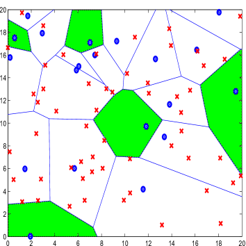
Figure 1: A channel realization for either M-MIMO or small-cell systems. Here “o”, “x”, and straight lines denote the transmitter (BS/DA), user, and boundaries between cells. The cells without any user are marked by green color.

III Massive MIMO System Analysis

In this section, we investigate the performance of M-MIMO systems based on the results in our paper [9, Section II]. First, we derive the distribution of the signal-to-interference-plus-noise ratio (SINR) and SIR. Note that if the UE intensity $\lambda_{u}$ is not sufficiently larger than $\lambda_{b}$, then some M-MIMO BSs may not possibly be associated to any UE, and thus, do not transmit signals. Therefore, it is necessary to study the transmission probability of each BS. The following result provides the area distribution of Voronoi cells.

Lemma 1 ([21])

Given a PPP $\Phi$ with homogeneous density $\lambda$. The probability distribution function (PDF) of $S$, the area of a typical Voronoi cell formed from $\Phi$, can be approximated as

$$f_{S}(x)\approx\frac{3.5^{3.5}}{\Gamma(3.5)}\lambda^{3.5}x^{2.5}e^{-3.5\lambda x}.$$ (3)

By using Lemma 1, the transmission probability of BSs is approximated as [22]

$$\epsilon_{C}\approx 1-\left(1+\frac{\lambda_{u}}{3.5\lambda_{b}}\right)^{-3.5}.$$ (4)

Note that given the transmission probability $\epsilon_{C}$, the transmitting BS locations are thus distributed according to a PPP $\widehat{\Phi}_{C,b}$ with density $\widehat{\lambda}_{C,b}$ $=\epsilon_{C}\lambda_{b}$.

III-A Conjugate Beamforming - Large System Analysis

Since all BSs employ conjugate beamforming, the transmit signal $\mbox{\boldmath{$x$}}_{C,b}$ is

$$\mbox{\boldmath{$x$}}_{C,b}=\mbox{\boldmath{$w$}}_{C,b}s_{C,b}=\frac{\sqrt{MP_{T}}\mbox{\boldmath{$h$}}_{C,b,b}}{\lVert\mbox{\boldmath{$h$}}_{C,b,b}\rVert}s_{C,b},$$ (5)

where $\mbox{\boldmath{$w$}}_{C,b}$ $=$ $\sqrt{MP_{T}}\mbox{\boldmath{$h$}}_{C,b,b}/\lVert\mbox{\boldmath{$h$}}_{C,b,b}\rVert$ $\in\mathbb{C}^{M\times 1}$ is the conjugate beamformer of BS $b$. As a consequence, the received signal of the UE associated to BS $b$ is given as follows

$$y_{C,b} =\sqrt{MP_{T}}\lVert\mbox{\boldmath{$h$}}_{C,b,b}\rVert s_{C,b}$$

$$+\displaystyle\sum_{b^{\prime}\in\mathcal{B}/\{b\}}\frac{\sqrt{MP_{T}}\mbox{\boldmath{$h$}}_{C,b^{\prime},b}^{H}\mbox{\boldmath{$h$}}_{C,b^{\prime},b^{\prime}}}{\lVert\mbox{\boldmath{$h$}}_{C,b^{\prime},b^{\prime}}\rVert}\mbox{\boldmath{$x$}}_{C,b^{\prime}}+n_{C,b},$$ (6)

The SINR of the UE associated to BS $b$ therefore can be expressed as

$$\text{SINR}_{b} =\frac{MP_{T}\lVert\mbox{\boldmath{$h$}}_{C,b,b}\rVert^{2}}{\sum\limits_{b^{\prime}\in\mathcal{B}/\{b\}}\displaystyle MP_{T}\frac{\mbox{\boldmath{$h$}}_{C,b^{\prime},b}^{H}\mbox{\boldmath{$h$}}_{C,b^{\prime},b^{\prime}}\mbox{\boldmath{$h$}}_{C,b^{\prime},b^{\prime}}^{H}\mbox{\boldmath{$h$}}_{C,b^{\prime},b}}{\lVert\mbox{\boldmath{$h$}}_{C,b^{\prime},b^{\prime}}\rVert^{2}}+\sigma_{n}^{2}}$$

$$=\frac{d_{C,b,b}^{-\mu}\left\lVert\widehat{\mbox{\boldmath{$h$}}}_{C,b,b}\right\rVert^{2}}{\sum\limits_{b^{\prime}\in\mathcal{B}/\{b\}}\displaystyle d_{C,b^{\prime},b}^{-\mu}\frac{\widehat{\mbox{\boldmath{$h$}}}_{C,b^{\prime},b}^{H}\widehat{\mbox{\boldmath{$h$}}}_{C,b^{\prime},b^{\prime}}\widehat{\mbox{\boldmath{$h$}}}_{C,b^{\prime},b^{\prime}}^{H}\widehat{\mbox{\boldmath{$h$}}}_{C,b^{\prime},b}}{\left\lVert\widehat{\mbox{\boldmath{$h$}}}_{C,b^{\prime},b^{\prime}}\right\rVert^{2}}+\frac{\sigma_{n}^{2}}{MP_{T}}}.$$ (7)

Note that the vector series $\frac{\widehat{\mbox{\boldmath{$h$}}}_{C,b,b}}{\sqrt{M}}$ $\in\mathbb{C}^{M\times 1}$ satisfy the condition of [16, Theorem 3.4]. Therefore, we have

$$\left\lVert\widehat{\mbox{\boldmath{$h$}}}_{C,b,b}\right\rVert^{2}/M\xrightarrow{M\to\infty}1,$$ (8)

Based on (8), the SINR of the UE associated to BS $b$ is expressed as

$$Q_{\text{M}}\triangleq\text{SINR}_{b}$$

$$=\frac{d_{C,b,b}^{-\mu}\left\lVert\widehat{\mbox{\boldmath{$h$}}}_{C,b,b}\right\rVert^{2}/M}{\sum\limits_{b^{\prime}\in\mathcal{B}/\{b\}}\displaystyle d_{C,b^{\prime},b}^{-\mu}\frac{\widehat{\mbox{\boldmath{$h$}}}_{C,b^{\prime},b}^{H}\widehat{\mbox{\boldmath{$h$}}}_{C,b^{\prime},b^{\prime}}\widehat{\mbox{\boldmath{$h$}}}_{C,b^{\prime},b^{\prime}}^{H}\widehat{\mbox{\boldmath{$h$}}}_{C,b^{\prime},b}}{M\left\lVert\widehat{\mbox{\boldmath{$h$}}}_{C,b^{\prime},b^{\prime}}\right\rVert^{2}}+\frac{\sigma_{n}^{2}}{M^{2}P_{T}}}$$

$$\xrightarrow{M\to\infty}\frac{Md_{C,b,b}^{-\mu}}{\sum\limits_{b^{\prime}\in\widehat{\Phi}_{C,d}/\{b\}}\displaystyle d_{C,b^{\prime},b}^{-\mu}|\tilde{h}_{b^{\prime}}|^{2}+\frac{\sigma_{n}^{2}}{MP_{T}}},$$ (9)

where $\tilde{h}_{b^{\prime}}\triangleq\frac{\widehat{\mbox{\boldmath{$h$}}}_{C,b^{\prime},b}^{H}\widehat{\mbox{\boldmath{$h$}}}_{C,b^{\prime},b^{\prime}}}{\left\lVert\widehat{\mbox{\boldmath{$h$}}}_{C,b^{\prime},b^{\prime}}\right\rVert}$; $\tilde{h}_{b^{\prime}}$’s are i.i.d. random variables each distributing as $\mathcal{CN}(0,1)$. The form (III-A) is similar to that investigated in [9, Section V]. It has been shown that (III-A) is difficult to study, in particular to derive the cumulative distribution probability (CDF) bounds. As discussed in [9, Section V], we can well approximate

$$\sum\limits_{b^{\prime}\in\widehat{\Phi}_{C,d}/\{b\}}\displaystyle d_{C,b^{\prime},b}^{-\mu}|\tilde{h}_{b^{\prime}}|^{2}\approx\sum\limits_{b^{\prime}\in\widehat{\Phi}_{C,d}/\{b\}}\displaystyle d_{C,b^{\prime},b}^{-\mu}.$$ (10)

As a consequence, we have

$$Q_{\text{M}}\approx\frac{Md_{C,b,b}^{-\mu}}{\sum\limits_{b^{\prime}\in\widehat{\Phi}_{C,d}/\{b\}}\displaystyle d_{C,b^{\prime},b}^{-\mu}+\frac{\sigma_{n}^{2}}{MP_{T}}}.$$ (11)

III-B Probability Distribution

We note that the form of the SINR in (11) is similar to that investigated in [9, Section II]. Therefore, we can apply the results for the outage probability, average achievable rate, and outage rate in [9, Section II] here. The only but important difference is that the interfering BSs’ locations are distributed according to the PPP $\widehat{\Phi}_{C,d}$ with density $\widehat{\lambda}_{d}$, while the PDF of the nearest distance follows that from PPP $\Phi_{C,d}$ with density $\lambda_{b}$. The following corollaries follow same reasonings as in [9, Theorem 1, (9), and (10)]. The proofs are given in Appendix A, where we only highlight the differences for brevity.

Corollary 1

Assume that the transmitting BSs follows a PPP $\widehat{\Phi}_{C,d}$ with density $\widehat{\lambda}_{C,d}$. The Laplace transform of $Q_{\text{M}}^{-1}$ can be expressed as

$$\mathcal{L}_{Q_{\text{M}}^{-1}}\left(s\right)=\pi\lambda_{b}\int_{0}^{\infty}\exp\bigg{\{}-\frac{sy^{\mu/2}\sigma_{n}^{2}}{M^{2}P_{T}}-\pi\widehat{\lambda}_{C,d}y$$

$$\left[1+\frac{1}{\epsilon_{C}}-e^{-s/M}+\left(\frac{s}{M}\right)^{2/\mu}\gamma\left(1-\frac{2}{\mu},\frac{s}{M}\right)\right]\bigg{\}}dy,$$ (12)

Corollary 2

Given that $M\to\infty$, the lower and upper bounds of the SIR distribution are given as follows

$$F^{\text{LB}}_{Q_{\text{M}}}(q)= 0, 0\leq q<M$$ , (13a)

$$F^{\text{LB}}_{Q_{\text{M}}}(q)= 1-\frac{1}{\epsilon_{C}M^{-\frac{2}{\mu}}q^{\frac{2}{\mu}}+1-\epsilon_{C}}, M\leq q$$ , (13b)

$$~{}~{}F^{\text{UB}}_{Q_{\text{M}}}(q) =1-\frac{1}{1+\epsilon_{C}\beta_{\text{n-fd}}M^{-2/\mu}q^{2/\mu}}.$$ (14)

Similar to [9, (10)], (14) is rigorously proved only for: (a) $q\geq M$, and (b) $q<M$ with $q\to 0$ or $q\to M$. The following result is a counterpart of [9, Corollary 1] for massive MIMO when $M\to\infty$. The proof can be deduced from Appendix A-B, and thus is omitted for brevity. Note that Corollary 3 does not require the approximation (10) since $\mathbb{E}_{\Phi}\left[M\text{SIR}_{b}^{-1}\right]$ already averages over the channel fading.

Corollary 3

Assuming a very large $M$, the expectation of $M\text{SIR}_{b}^{-1}$ is given as $\mathbb{E}_{\Phi}\left[M\text{SIR}_{b}^{-1}\right]=\frac{2\epsilon_{C}}{\mu-2}$.

Remark 1

It is important to remind that Corollaries 2 and 3 are derived by assuming that the noise power is negligible, i.e., $\sigma^{2}=0$, and considering the SIR instead of SINR. In small UE density network, i.e., $\lambda_{b}\gg\lambda_{u}$, such assumption is not accurate anymore since the interfering sources are far away and the interfering power is small. The noise effect therefore is more important. As a consequence, Corollaries 2 and 3 are not accurate in UE-sparse networks. Further results for M-MIMO with asymptotically small UE density will be presented in Section III-D.

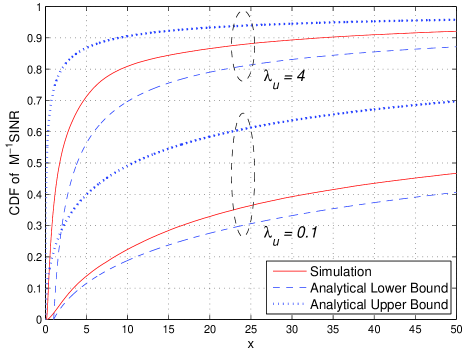
Figure 2: Simulated SINR CDF and its bounds (13b), (14) for M-MIMO with $M=64$, $\mu=3.7$, $\lambda_{b}=1$, and $P_{T}/\sigma^{2}=15$ dB.

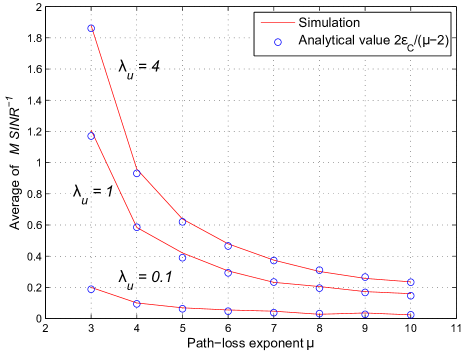
Figure 3: Average of $M\text{SINR}_{b}^{-1}$ for M-MIMO with $M=64$, $\mu=3.7$, $\lambda_{b}=1$, and $P_{T}/\sigma^{2}=15$ dB.

In Figs. 2 and 3, we confirm the validity of Corollaries 2 and 3, respectively. From Fig. 3, it is observed that the assumption that the transmitting BSs follow a PPP $\widehat{\Phi}_{C,d}$ with density $\widehat{\lambda}_{C,d}=\epsilon_{C}\lambda_{b}$ with $\epsilon_{C}$ given in (4) is quite accurate. However, the upper bound is only close to the exact SINR distribution when $\lambda_{u}$ is sufficiently large ($\lambda_{u}\geq\lambda_{b}$ by intensive simulations), as shown in Fig. 2. As $\lambda_{u}$ decreases compared to $\lambda_{b}$, the upper bound (14) becomes looser. The reason is that some inequalities, used to derive the upper bound in Appendix A-B, are not strict especially when $\epsilon_{C}$ is small. The lower bound, however, is not affected by the UE density due to its simple derivation.

III-C Average Achievable and Outage Rate

Based on Corollary 2, we investigate the average Shannon and outage rates for M-MIMO systems. We note that due to TDMA/FDMA, each user is only served for a fraction of time or a sub-band. Assuming that all users have the same transmission priority, that fraction can be defined as $\frac{1}{N_{b,u}}$, where $N_{b,u}$ is the number of users in cell $b$. The following result establishes $\mathbb{E}\left[N_{b,u}\right]$.

Lemma 2

The expectation of the number of users in a typical cell $b$ is given as

$$\mathbb{E}\left[N_{b,u}\right]=\frac{\lambda_{C,u}}{\lambda_{C,b}}=\frac{\lambda_{u}}{\lambda_{b}}.$$ (15)

Proof:

Please refer to Appendix B. ∎

As expected, the average number of users in a cell is proportional to the UE density while inversely proportional to the BS density. The simple linear scaling is surprising, but intuitive. The reason is due to the homogeneity of both BS and UE PPPs, which does not create clusters of either BSs or UEs. Therefore, with $\lambda_{u}$ UEs and $\lambda_{b}$ BSs in a region of $1$ km², we expect to see the UEs homogeneously distributed across all BSs, which leads to $\lambda_{u}/\lambda_{b}$. By comparing the simulated and analytical values of $\mathbb{E}\left[N_{b,u}\right]$, intensive simulations confirm the validity of Lemma 2. The comparison is not presented due to the space constraint.

Note that the rate of an UE associated to BS $b$ is given as

$$R_{b,u}=\frac{1}{N_{b,u}}\log_{2}\left(1+\text{SINR}_{b}\right),$$ (16)

where the fraction $\frac{1}{N_{b,u}}$ is due to TDMA/FDMA. We thus obtain the average Shannon rate of a typical user as follows

$$R_{\text{M}}=\mathbb{E}_{\Phi_{C,b},\Phi_{C,u}}\left[R_{b,u}\right]\overset{(a)}{=}\mathbb{E}\left[\frac{1}{N_{b,u}}\right]\mathbb{E}\left[\log_{2}\left(1+\text{SINR}_{b}\right)\right].$$ (17)

Here, $(a)$ is due to TDMA/FDMA and the fact that the random variables $\text{SINR}_{b}$ and $N_{b,u}$ are independent given that TDMA/FDMA is applied.

Based on Corollary 2 and Lemma 2, we can derive the bounds for the average achievable rate and the outage rate as follows. The proofs are similar to that of [9, Lemmas 3 and 4] and omitted for brevity.

Corollary 4

The average user rate $R_{\text{M}}$ is bounded above and below by $R^{\text{UB}}_{\text{M}}$ and $R^{\text{LB}}_{\text{M}}$, respectively, where

$$R^{\text{UB}}_{\text{M}} =\min\left\{1,\frac{\lambda_{b}}{\lambda_{u}}\right\}\Bigg{(}\log_{2}(1+M)$$

$$+\int_{\log_{2}(1+M)}^{\infty}\frac{dt}{\epsilon_{C}M^{-2/\mu}(2^{t}-1)^{2/\mu}+1-\epsilon_{C}}\Bigg{)},$$ (18)

$$R^{\text{LB}}_{\text{M}}=\min\left\{1,\frac{\lambda_{b}}{\lambda_{u}}\right\}\int_{0}^{\infty}\frac{dt}{1+\epsilon_{C}\beta_{\text{n-fd}}M^{-2/\mu}(2^{t}-1)^{2/\mu}}.$$ (19)

Corollary 5

The outage user rate $\text{OR}_{\text{M}}(\eta)$ is upper- and lower-bounded by $\text{OR}_{\text{M}}^{\text{UB}}(\eta)$ and $\text{OR}_{\text{M}}^{\text{LB}}(\eta)$, respectively, where
$\text{OR}_{\text{M}}^{\text{UB}}(\eta)$

$$= \min\left\{1,\frac{\lambda_{b}}{\lambda_{u}}\right\}\log_{2}(1+\eta), 0\leq\eta\leq M$$ , (20a)

$$= \min\left\{1,\frac{\lambda_{b}}{\lambda_{u}}\right\}\frac{\log_{2}(1+\eta)}{\epsilon_{C}\left(\frac{\eta}{M}\right)^{2/\mu}+1-\epsilon_{C}}, M<\eta$$ . (20b)

$$\text{OR}^{\text{LB}}_{\text{M}}(\eta) =\min\left\{1,\frac{\lambda_{b}}{\lambda_{u}}\right\}\frac{\log_{2}\left(1+\eta\right)}{1+\epsilon_{C}\beta_{\text{n-fd}}\left(\frac{\eta}{M}\right)^{2/\mu}}.$$ (21)

Here, the term $\min\left\{1,\frac{\lambda_{b}}{\lambda_{u}}\right\}$ in Corollaries 4 and 5 is due to the fact that TDMA is applied only when $N_{b,u}>1$, and we have approximated

$$\mathbb{E}\left[\frac{1}{N_{b,u}}\right]\approx\frac{1}{\mathbb{E}\left[N_{b,u}\right]}=\frac{\lambda_{b}}{\lambda_{u}}.$$ (22)

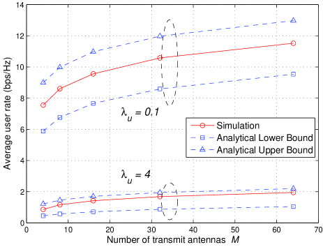
Figure 4: Average user rate and its bounds (4) and (19) for M-MIMO with respect to $M$. Here, $\mu=3.7$, $\lambda_{b}=1$, and $P_{T}/\sigma^{2}=15$ dB.

In Figs. 4 and 5, we compare the average and outage user rates with the bounds given in (4)-(21). We first observe that the scaling laws of the bounds are closely matched with the true rates. The gap, however, seems to increase as the UE-BS density ratio becomes smaller. Nevertheless, the bounds are useful for further studies on the M-MIMO performance under various network models.

III-D Asymptotically Small UE Density

In this section, we investigate the performance of M-MIMO under the asymptotically small UE density regime. As the transmission probability $\epsilon_{C}$ approaches $0$, the interference also goes to $0$ since the interfering BSs are farther apart from each other. In such cases, we can ignore the interference but not the noise due to its dominant effect. The SINR can now be approximated as the SNR and expressed as

$$Q_{\text{M}}=\text{SINR}_{b}\approx\text{SNR}_{b} =\frac{MP_{T}d_{C,b,b}^{-\mu}\left\lVert\widehat{\mbox{\boldmath{$h$}}}_{C,b,b}\right\rVert^{2}}{\sigma_{n}^{2}}$$

$$\xrightarrow{a.s.}\frac{M^{2}P_{T}d_{C,b,b}^{-\mu}}{\sigma_{n}^{2}}.$$ (23)

Since the PDF of $d_{C,b,b}$ is

$$f_{D_{C,b,b}}(x)=2\pi\lambda_{b}xe^{-\pi\lambda_{b}x^{2}},$$ (24)

it is straightforward to derive the SINR distribution as follows

$$\text{Pr}\left\{Q_{\text{M}}\leq q\right\} =\text{Pr}\left\{d_{C,b,b}\geq\left(\frac{M^{2}P_{T}}{q\sigma_{n}^{2}}\right)^{1/\mu}\right\}$$

$$=\exp\left(-\pi\lambda_{b}\frac{M^{4/\mu}P_{T}^{2/\mu}}{\sigma_{n}^{4/\mu}q^{2/\mu}}\right).$$ (25)

Therefore, the average Shannon and outage rates are given as

$$R_{\text{M}}=\int_{0}^{\infty}\left[1-\exp\left(-\pi\lambda_{b}\frac{M^{4/\mu}P_{T}^{2/\mu}}{\sigma_{n}^{4/\mu}(2^{t}-1)^{2/\mu}}\right)\right]dt,$$ (26)

$$\text{OR}_{\text{M}}(\eta)=\log_{2}(1+\eta)\left[1-\exp\left(-\pi\lambda_{b}\frac{M^{4/\mu}P_{T}^{2/\mu}}{\sigma_{n}^{4/\mu}\eta^{2/\mu}}\right)\right].$$ (27)

Figure 5: Outage rate and its bounds (20b) and (21) for M-MIMO with $M=64$, $\mu=3.7$, $\lambda_{b}=1$, and $P_{T}/\sigma^{2}=15$ dB.

IV Small-Cell System Analysis

Similar to M-MIMO, if the UE intensity $\lambda_{u}$ is not sufficiently larger than $\lambda_{b}$, then some DAs in the small-cell system may not be associated to any UE, and thus, do not transmit signals. Applying Lemma 1, we can derive the transmission probability of a DA in our system as [22]

$$\epsilon_{D}\approx 1-\left(1+\frac{\lambda_{u}}{3.5M\lambda_{b}}\right)^{-3.5}.$$ (28)

The transmitting DAs thus can be modeled as a homogeneous PPP $\widehat{\Phi}_{D,b}$ obtained by thinning the DA PPP $\Phi_{D,b}$ with a probability $\epsilon_{D}$ that DA is activated. In this case, the SINR of a typical UE $k$ can be described as

$$Q_{\text{SM}}\triangleq\frac{\big{|}\widehat{h}_{D,k,k}\big{|}^{2}d_{k,k}^{-\mu}P_{T}}{\sum_{k^{\prime}\in\Phi_{D,b}/\{k\}}^{K}{\big{|}\widehat{h}_{k,k^{\prime}}\big{|}^{2}P_{T}}{d_{k,k^{\prime}}^{-\mu}}+\sigma_{n}^{2}}.$$ (29)

Using $\epsilon_{D}$, we can obtain the coverage probability of a typical user $k$ in Lemma 3 [23].

Lemma 3 ([23])

Given that the transmitting DAs are modeled as PPP $\widehat{\Phi}_{D,b}$ and both desired and interfering signals obey Rayleigh distribution, the coverage probability for user $k$ is expressed as

$$\Pr\left(Q_{\text{SM}}\geq q\right) =\pi M\lambda_{b}\int_{0}^{\infty}\exp\bigg{\{}-\frac{\sigma_{n}^{2}}{P_{T}}qv^{\mu/2}$$

$$-\pi M\lambda_{b}v\left[1+\epsilon_{D}q^{2/\mu}\rho\left(q^{-2/\mu},\frac{\mu}{2}\right)\right]\bigg{\}}dv.$$ (30)

A direct corollary of Lemma 6 is the SIR distribution for the case $\sigma_{n}^{2}/P_{T}=0$ given as follows.

Corollary 6

The SIR distribution of a small cell system is given as

$$F_{Q_{\text{SM}}}(q)=1-\frac{1}{1+\epsilon_{D}q^{2/\mu}\rho\left(q^{-2/\mu},\frac{\mu}{2}\right)}.$$ (31)

Again, we obtain the SIR CDF, average achievable rate, and outage rate bounds for the small-cell system. The differences between the following Corollaries 7, 8 and [9, Lemma 6] are that the interfering cells follows a PPP with density $\epsilon_{D}\lambda_{b}$, and each DA might need to serve multiple UEs via TDMA/FDMA. We note that the expectation of the number of UEs associated with a typical DA $k$ is given as (cf. Lemma 2)

$$\mathbb{E}\left[N_{k,u}\right]=\frac{\lambda_{D,u}}{\lambda_{D,b}}=\frac{\lambda_{u}}{M\lambda_{b}}.$$ (32)

The proofs for the following results are similar to those of [9, Lemmas 5 and 6], and thus omitted for brevity.

Corollary 7

The lower and upper bounds for the distribution of $Q_{\text{SM}}$ defined in (29) are given as

$$F^{\text{LB}}_{Q_{\text{SM}}}(q) =1-\mathbb{E}_{h}\left[\frac{1}{1+\frac{2\epsilon_{D}q^{2/\mu}}{\mu|h|^{2/\mu}}\Gamma\left(\frac{2}{\mu},\frac{|h|^{2}}{q}\right)}\right],$$ (33)

$$F^{\text{UB}}_{Q_{\text{SM}}}(q) =1-\frac{1}{1+\epsilon_{D}\beta_{\text{fd}}q^{2/\mu}},$$ (34)

where $|h|^{2}$ is exponentially distributed.

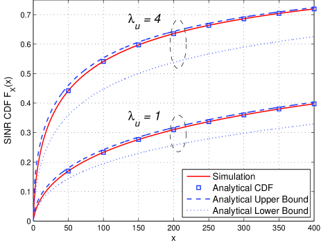
Figure 6: Simulated SINR distribution, analytical result (31), and bounds (33), (34) for small-cell system with $\lambda_{D,b}=M\lambda_{b}=64$, $\mu=3.7$, and $P_{T}/\sigma^{2}=15$ dB.

Corollary 8

The average Shannon rate $R_{\text{SM}}(\alpha)$ and the outage rate $\text{OR}_{\text{SM}}(\alpha,\eta)$ are bounded below, respectively, by

$$R^{\text{LB}}_{\text{SM}} =\min\left\{1,\frac{M\lambda_{b}}{\lambda_{u}}\right\}\int_{0}^{\infty}\frac{dt}{1+\epsilon_{D}\beta_{\text{fd}}\left(2^{t}-1\right)^{2/\mu}},$$ (35)

$$\text{OR}^{\text{LB}}_{\text{SM}}(\eta) =\min\left\{1,\frac{M\lambda_{b}}{\lambda_{u}}\right\}\frac{\log_{2}\left(1+\eta\right)}{1+\epsilon_{D}\beta_{\text{fd}}\eta^{2/\mu}}.$$ (36)

Again, the term $\min\left\{1,\frac{M\lambda_{b}}{\lambda_{u}}\right\}$ is due to the fact that TDMA/FDMA is applied only when $N_{k,u}>1$, and we have approximated

$$\frac{1}{N_{k,u}}\approx\frac{1}{\mathbb{E}\left[N_{k,u}\right]}=\frac{M\lambda_{b}}{\lambda_{u}}.$$ (37)

In Fig. 6, we compare the SINR distribution, analytical result (31), and bounds (33), (34) for two small-cell systems. It is observed that the upper-bound (34), although simple, is quite tight when compared with the lower-bound (33). Figs. 7 and 8 illustrate the average and outage user rate for various small-cell systems. We also show the analytical rate lower bounds given in Corollary 8 for comparison. In contrast to the M-MIMO case, the bounds for small-cell systems are quite tight. Note that we do not derive and present the analytical upper bounds for the rates here since they are complicated and of limited use for subsequent analyses.

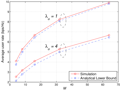
Figure 7: Average user rate and its lower bound (35) with respect to $M$ for small-cell system. Here, $\lambda_{b}=1$, $\mu=3.7$, $P_{T}/\sigma^{2}=15$ dB, and $\lambda_{D,b}=M\lambda_{b}$.

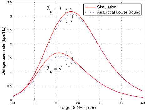
Figure 8: Outage rate and its lower bound (36) for small-cell system with $\lambda_{D,b}=M\lambda_{b}=16$, $\mu=3.7$, and $P_{T}/\sigma^{2}=15$ dB.

IV-A Asymptotically Small UE Density

Under the asymptotically small UE density regime, the interference is negligible and the SINR of small-cell system can be expressed as

$$Q_{\text{SM}}=\text{SINR}_{k}\approx\text{SNR}_{k}=\frac{\big{|}\widehat{h}_{D,k,k}\big{|}^{2}d_{k,k}^{-\mu}P_{T}}{\sigma_{n}^{2}}.$$ (38)

Since the PDF of $d_{k,k}$ is

$$f_{D_{k,k}}(x)=2\pi M\lambda_{b}xe^{-\pi M\lambda_{b}x^{2}},$$ (39)

it is straightforward to derive the SINR distribution as follows

$$\text{Pr}\left\{Q_{\text{SM}}\leq q\right\} =\mathbb{E}_{h}\left[\exp\left(-\pi M\lambda_{b}\frac{P_{T}^{2/\mu}|h|^{2/\mu}}{\sigma_{n}^{4/\mu}q^{2/\mu}}\right)\right],$$ (40)

where the random variable $h\sim\mathcal{CN}(0,1)$.

Therefore, the average Shannon and outage rate are

$$R_{\text{SM}}=\int_{0}^{\infty}\left(1-\mathbb{E}_{h}\left[\exp\left(-\pi M\lambda_{b}\frac{P_{T}^{2/\mu}|h|^{2/\mu}}{\sigma_{n}^{4/\mu}(2^{t}-1)^{2/\mu}}\right)\right]\right)dt,$$ (41)

$$\text{OR}_{\text{SM}}(\eta)$$

$$=\log_{2}(1+\eta)\left(1-\mathbb{E}_{h}\left[\exp\left(-\pi M\lambda_{b}\frac{P_{T}^{2/\mu}|h|^{2/\mu}}{\sigma_{n}^{4/\mu}\eta^{2/\mu}}\right)\right]\right).$$ (42)

To derive the bounds for (40)-(IV-A), we note that the function $\exp(-\alpha x^{\beta})$ with $\beta\leq 1$ is convex in $x>0$. Therefore, applying Jensen’s inequality, we obtain

$$F_{Q_{\text{SM}}}(q) \geq\exp\left(-\pi M\lambda_{b}\frac{P_{T}^{2/\mu}\mathbb{E}_{h}\left[|h|^{2/\mu}\right]}{\sigma_{n}^{4/\mu}q^{2/\mu}}\right)$$

$$=\exp\left(-\pi M\lambda_{b}\frac{P_{T}^{2/\mu}\Gamma(1+\frac{2}{\mu})}{\sigma_{n}^{4/\mu}q^{2/\mu}}\right)\triangleq F^{\text{LB}}_{Q_{\text{SM}}}(q).$$ (43)

The upper bounds for $R_{\text{SM}}$ and $\text{OR}_{\text{SM}}(\eta)$ are therefore given as

$$R_{\text{SM}}^{\text{UB}}=\int_{0}^{\infty}\left(1-\exp\left(-\pi M\lambda_{b}\frac{P_{T}^{2/\mu}\Gamma(1+\frac{2}{\mu})}{\sigma_{n}^{4/\mu}(2^{t}-1)^{2/\mu}}\right)\right)dt,$$ (44)

$$\text{OR}_{\text{SM}}^{\text{UB}}(\eta)$$

$$=\log_{2}(1+\eta)\left(1-\exp\left(-\pi M\lambda_{b}\frac{P_{T}^{2/\mu}\Gamma(1+\frac{2}{\mu})}{\sigma_{n}^{4/\mu}q^{2/\mu}}\right)\right).$$ (45)

V Rate Comparison for M-MIMO and Small-Cell Systems

M-MIMO and small-cell represent two densification approaches in 5G communication systems. The lack of a performance comparison between them is even more surprising given the fact that each approach has attracted significant attention in the literature. In this section, we exploit the newly obtained results in Sections III and IV to draw several observations on M-MIMO and small-cell networks, revealing which approach is better and under which setup. Here, the metric is the outage rate for simple arguments, but our observations can be readily extended to the average Shannon rate. The key parameter here is the UE density $\lambda_{u}$.

V-A Very Large UE Density: $\lambda_{u}\geq M\lambda_{b}$

In this case, the lower bounds of the outage rate are reduced to

$$\text{OR}^{\text{LB}}_{\text{M}}(\eta)=\frac{\lambda_{b}}{\lambda_{u}}\frac{\log_{2}\left(1+\eta\right)}{1+\epsilon_{C}\beta_{\text{n-fd}}M^{-2/\mu}\eta^{2/\mu}},$$ (46)

$$\text{OR}^{\text{LB}}_{\text{SM}}(\eta)=\frac{M\lambda_{b}}{\lambda_{u}}\frac{\log_{2}\left(1+\eta\right)}{1+\epsilon_{D}\beta_{\text{fd}}\eta^{2/\mu}},$$ (47)

where $\epsilon_{C}\approx 1-\left(1+\frac{\lambda_{u}}{3.5\lambda_{b}}\right)^{-3.5}\approx 1$. Simple manipulation shows that $\text{OR}^{\text{LB}}_{\text{SM}}(\eta)\geq\text{OR}^{\text{LB}}_{\text{M}}(\eta)$ iff

$$M+M^{1-2/\mu}\epsilon_{C}\beta_{\text{n-fd}}\eta^{2/\mu}\geq 1+\epsilon_{D}\beta_{\text{fd}}\eta^{2/\mu}.$$ (48)

As a loose approximation, (48) holds if $M^{1-2/\mu}\epsilon_{C}\beta_{\text{n-fd}}\geq\epsilon_{D}\beta_{\text{fd}}$, which is true since $\beta_{\text{n-fd}}>\beta_{\text{fd}}$, $\epsilon_{C}\approx 1\geq\epsilon_{D}$, and $M$ is large. We thus observe that a small-cell system outperforms a M-MIMO counterpart when the UE density is very large. This is due to the effect of multiplexing large number of users under TDMA/FDMA, which diminishes the interference-mitigation benefit of M-MIMO.

V-B Intermediate UE density: $\lambda_{b}<\lambda_{u}<M\lambda_{b}$

Since $\frac{\lambda_{u}}{3.5M\lambda_{b}}$ is small, we have

$$\epsilon_{D}\approx 1-\left(1+\frac{\lambda_{u}}{3.5M\lambda_{b}}\right)^{-3.5}\approx\frac{\lambda_{u}}{M\lambda_{b}}.$$ (49)

Based on (21) and (36), we can express the outage rates as

$$\text{OR}^{\text{LB}}_{\text{M}}(\eta)=\frac{\lambda_{b}}{\lambda_{u}}\frac{\log_{2}\left(1+\eta\right)}{1+\epsilon_{C}\beta_{\text{n-fd}}M^{-2/\mu}\eta^{2/\mu}},$$ (50)

$$\text{OR}^{\text{LB}}_{\text{SM}}(\eta)=\frac{\log_{2}\left(1+\eta\right)}{1+\epsilon_{D}\beta_{\text{fd}}\eta^{2/\mu}}.$$ (51)

The condition for $\text{OR}^{\text{LB}}_{\text{SM}}(\eta)\geq\text{OR}^{\text{LB}}_{\text{M}}(\eta)$ is

$$1+\frac{1}{M^{2/\mu}}\epsilon_{C}\beta_{\text{n-fd}}\eta^{2/\mu}\geq\frac{\lambda_{b}}{\lambda_{u}}+\frac{1}{M}\beta_{\text{fd}}\eta^{2/\mu}.$$ (52)

We note that (52) is true since $1\geq\frac{\lambda_{b}}{\lambda_{u}}$ and $M\geq M^{2/\mu}$. Therefore, s small-cell system outperforms a M-MIMO counterparts when the UE density is moderate. Similar to Section V-A, the reason is again due to the effect of multiplexing a large number of users under TDMA/FDMA M-MIMO.

Remark 2

In Sections V-A and V-B, a stronger and stricter result which states that $\text{OR}^{\text{LB}}_{\text{SM}}(\eta)\geq\text{OR}^{\text{UB}}_{\text{M}}(\eta)$ is also provable using the same arguments. However, we have used the lower bounds $\text{OR}^{\text{LB}}_{\text{M}}(\eta)$ instead due to the symmetry and for the ease of explanation.

V-C Asymptotically Small UE Density: $\lambda_{u}\ll\lambda_{b}$

Assuming a small UE density, it is difficult to compare M-MIMO and small-cell systems since the M-MIMO lower bounds are not close to the exact distribution or rates. In this subsection, we consider the asymptotic regime where $\lambda_{u}$ is very small compared to $\lambda_{b}$ to reveal some insights for the small UE density case. Note that

$$\exp\left(-\frac{\pi\lambda_{b}P_{T}^{2/\mu}}{\sigma_{n}^{4/\mu}q^{2/\mu}}M^{4/\mu}\right)\leq\exp\left(-\frac{\pi\lambda_{b}P_{T}^{2/\mu}}{\sigma_{n}^{4/\mu}q^{2/\mu}}M\Gamma\Big{(}1+\frac{2}{\mu}\Big{)}\right),$$ (53)

when $\mu<4$ and $M$ is large enough, i.e., $M^{\frac{4}{\mu}-1}>\Gamma\Big{(}1+\frac{2}{\mu}\Big{)}$. From (26), (27), (44), and (IV-A), it is straightforward to prove that $R_{\text{M}}\geq R^{\text{UB}}_{\text{SM}}$ and $\text{OR}_{\text{M}}(\eta)\geq\text{OR}^{\text{UB}}_{\text{SM}}(\eta)$.

The above result essentially asserts that M-MIMO outperforms small-cell densification, albeit when the UE density is asymptotically small and $\mu<4$. Combined with observations from Sections V-A and V-B, we note that there exists a threshold with smaller UE density than which we should employ M-MIMO and larger UE density than which small-cell densification is more preferable, in terms of spectral efficiency. As an example, we compare the achievable user rates of M-MIMO and small-cell systems in Fig. 9. Note that as the path-loss exponent $\mu$ approaches $4$, $\lambda_{u}$ needs to be smaller so that M-MIMO rate can outperform small-cell counterpart. When $\mu\geq 4$, the M-MIMO rate is always worse than that of small-cell, as suggested by (53).

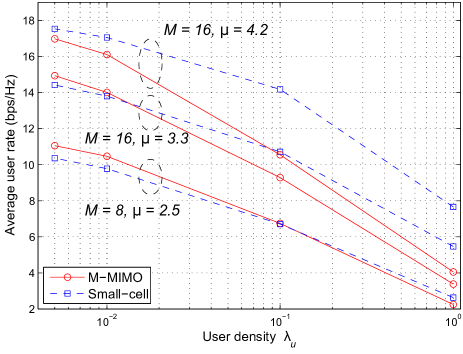
Figure 9: Comparison of the achievable user rate between M-MIMO and small-cell systems with $\lambda_{b}=1$.

We would like to highlight here that our study have not considered the deployment cost, the signaling overhead, the handover implementation, etc. We have also not considered multiuser beamforming in M-MIMO. Due to the space constraint, we leave such interesting and important investigations as our future works.

Note that we can consider small-cell and M-MIMO systems as two extrema of a balancing problem, where the number of BS antennas and BS density can vary while their product always equals to $M\lambda_{b}$. In other words, the problem is to distribute the antennas from a pool with density $M\lambda_{b}$ so that the resulting rate performance is optimal. The analysis of this problem is partially covered by Sections III and IV. The above arguments suggest that the optimal setup should be a moderate M-MIMO system with sufficient beamforming gain and a sufficiently dense BS deployment.

VI Energy Efficiency Comparison for M-MIMO and Small-Cell Systems

Apart from spectral efficiency, energy efficiency (EE) is also an important factor for evaluating future communications networks due to several environmental concerns. In this section, we compare M-MIMO and small-cell systems using EE as the metric. In the literature, a conventional definition for EE is

$$\text{EE}\triangleq\frac{R_{\text{AP/BS}}}{P_{\text{AP/BS}}},$$ (54)

where $P_{\text{AP/BS}}$ and $R_{\text{AP/BS}}$ are the transmit power and sum-rate of the corresponding AP/BS to all users, respectively. However, for ease of analysis, we consider the following EE definition based on the outage rate

$$\text{EE}(\eta)\triangleq\frac{\text{OR}_{\text{AP/BS}}(\eta)}{P_{\text{AP/BS}}}.$$ (55)

We can interpret $\text{EE}(\eta)$ as the energy efficiency of the AP/BS given that the user SINR satisfies the constraint SINR $\geq\eta$. Observations for EE based on (54) can be similarly obtained. Note that due to the transmission probability, the expected transmission power for each M-MIMO BS and small-cell AP are given as $\epsilon_{C}MP_{T}$ and $\epsilon_{D}P_{T}$, respectively. We first consider the moderate to large UE density regime where $\lambda_{b}<\lambda_{u}$ and obtain

$$\text{EE}^{\text{LB}}_{\text{SM}}(\eta)=\frac{\text{OR}^{\text{LB}}_{\text{SM}}(\eta)}{\epsilon_{D}P_{T}}>\frac{\text{OR}^{\text{LB}}_{\text{M}}(\eta)}{\epsilon_{D}P_{T}}\gg\frac{\text{OR}^{\text{LB}}_{\text{M}}(\eta)}{\epsilon_{C}MP_{T}}=\text{EE}^{\text{LB}}_{\text{M}}(\eta),$$ (56)

since $\epsilon_{D}<\epsilon_{C}$, $M\gg 1$, and $\text{OR}^{\text{LB}}_{\text{SM}}(\eta)>\text{OR}^{\text{LB}}_{\text{M}}(\eta)$ from Sections V-A and V-B.

Furthermore, under the asymptotically small UE density regime with $\lambda_{u}\ll\lambda_{b}$, we have $\epsilon_{C}\approx\frac{\lambda_{u}}{\lambda_{b}}$ and $\epsilon_{D}\approx\frac{\lambda_{u}}{M\lambda_{b}}$. Therefore, $\epsilon_{C}\gg\epsilon_{D}$. From (26), (27), (41), and (IV-A), it is straightforward to show that $\text{EE}_{\text{SM}}>\text{EE}_{\text{M}}$ and $\text{EE}_{\text{SM}}(\eta)>\text{EE}_{\text{M}}(\eta)$ by noting that the exponential function approaches $0$ as $M$ grows large.

The above result reveals that small-cell systems are more energy-efficient than M-MIMO counterparts with large, moderate, or asymptotically small UE densities. Strictly speaking, such results do not cover the small UE density regime. However, we conjecture that small cells outperforms M-MIMO in terms of EE under all cases. This conclusion is likely to hold even with multiuser beamforming/precoding applied at each M-MIMO BS.

From Sections V and VI, we observe another important aspect of the trade-off between M-MIMO and small-cell densification. Particularly, even through M-MIMO have a higher spectral efficiency as under small UE density regime, small-cell densification might still be a preferable option for certain communication systems due to its higher EE performance.

VII Conclusions

In this paper, we have compared the spectral and energy efficiencies of massive MIMO and small-cell systems. Particularly, we have derived SIR distribution bounds for both systems, based on which the average Shannon and outage rate bounds are obtained. We have also analyzed the performance of M-MIMO and small-cell under asymptotically small UE density regime, which represents UE-sparse networks. The M-MIMO and small-cell systems were then compared in terms of spectral and energy efficiencies. For the rate performance, we observe that M-MIMO surpasses small-cell densification when the UE density is small compared with BS/AP density and number of antennas, and vice versa. However, small-cell network yields better energy efficiency than M-MIMO counterpart under all cases. The results of this paper are useful for the optimal design of practical 5G networks and other 5G system performance analyses.

Appendix A Proof of Corollaries 1 and 2

A-A Proof of Corollary 1

Given that $d_{C,b,b}=x$. The Laplace transform is given as [9, (26)]

$$\mathcal{L}_{Q_{\text{M}}^{-1}}\left(s|d_{C,b,b}=x\right)=e^{-\frac{s}{M}x^{\mu}\delta}\exp\bigg{\{}-\pi\widehat{\lambda}_{C,b}x^{2}(1-e^{-s/M})$$

$$\qquad\qquad-\pi\widehat{\lambda}_{C,b}\left(\frac{s}{M}\right)^{2/\mu}x^{2}\gamma\left(1-\frac{2}{\mu},\frac{s}{M}\right)\bigg{\}},$$ (57)

where $\delta=\frac{\sigma_{n}^{2}}{MP_{T}}$. Now we observe that $d_{C,b,b}$ is the distance from an arbitrary origin to the nearest point of a PPP with density $\lambda_{b}$. The PDF of $d_{C,b,b}$ is expressed as follows

$$f_{D_{C,b,b}}(x)=2\pi\lambda_{b}xe^{-\pi\lambda_{b}x^{2}}.$$ (58)

The Laplace transform of $\text{SINR}_{b}^{-1}$ is thus obtained as

$$\mathcal{L}_{Q_{\text{M}}^{-1}}\left(s\right)$$

$$=\int_{0}^{\infty}\mathcal{L}_{\text{SINR}^{-1}}\left(s|d_{C,b,b}=x\right)f_{D_{C,b,b}}(x)dx$$

$$=2\pi\lambda_{b}\int_{0}^{\infty}x\exp\bigg{\{}-\frac{s}{M}x^{\mu}\delta-\pi\widehat{\lambda}_{C,b}x^{2}\bigg{[}1+\frac{\lambda_{b}}{\widehat{\lambda}_{C,b}}$$

$$\qquad\qquad-e^{-s/M}+\left(\frac{s}{M}\right)^{2/\mu}\gamma\left(1-\frac{2}{\mu},\frac{s}{M}\right)\bigg{]}\bigg{\}}dx$$

$$=\pi\lambda_{b}\int_{0}^{\infty}\exp\bigg{\{}-\frac{sy^{\mu/2}\sigma_{n}^{2}}{M^{2}P_{T}}-\pi\widehat{\lambda}_{C,b}y\bigg{[}1+\frac{1}{\epsilon_{C}}$$

$$\qquad\qquad-e^{-s/M}+\left(\frac{s}{M}\right)^{2/\mu}\gamma\left(1-\frac{2}{\mu},\frac{s}{M}\right)\bigg{]}\bigg{\}}dy.$$ (59)

This concludes the proof of Corollary 1.

A-B Proof of Corollary 2

For ease of presentation, we will consider $Q_{\text{M}}/M$. The lower bound is given as

$$F^{\text{LB}}_{Q_{\text{M}}/M}(q) =\int_{0}^{\infty}F^{\text{LB}}_{Q_{M}/M}(q|d_{C,b,b}=x)f_{D_{C,b,b}}(x)dx$$

$$=\int_{0}^{\infty}\left(1-e^{-\widehat{\lambda}_{C,b}\pi\left(q^{2/\mu}-1\right)x^{2}}\right)2\pi\lambda_{b}xe^{-\pi\lambda_{b}x^{2}}dx$$

$$=1-\frac{1}{\epsilon_{C}q^{2/\mu}+1-\epsilon_{C}}.$$ (60)

Now assume that $d_{C,b,b}=x$, $q\geq 1$, and $\xi\geq 1$. Similar to [9, (39)], the distribution for massive MIMO case can be bounded as

$$F_{Q_{\text{M}}/M}(q|d_{C,b,b}=x)\leq 1-e^{-\widehat{\lambda}_{C,b}\pi\left((\xi q)^{2/\mu}-1\right)x^{2}}$$

$$\qquad+e^{-\widehat{\lambda}_{C,b}\pi\left((\xi q)^{2/\mu}-1\right)x^{2}}\frac{2\pi\widehat{\lambda}_{C,b}x^{2}\xi^{2/\mu-1}q^{2/\mu}}{\mu-2},$$ (61)

We therefore obtain

$$F_{Q_{\text{M}}/M}(q)$$

$$\leq 2\pi\lambda_{b}\int_{0}^{\infty}\left(1-e^{-\widehat{\lambda}_{C,b}\pi\left((\xi q)^{2/\mu}-1\right)x^{2}}\right)xe^{-\pi\lambda_{b}x^{2}}dx$$

$$+\frac{(2\pi\lambda_{b})^{2}\epsilon_{C}\xi^{2/\mu-1}q^{2/\mu}}{\mu-2}\int_{0}^{\infty}x^{3}e^{-\pi\lambda_{b}\left(\epsilon_{C}(\xi q)^{2/\mu}+1-\epsilon_{C}\right)x^{2}}dx$$

$$=1-\frac{1}{\epsilon_{C}(\xi q)^{2/\mu}+1-\epsilon_{C}}$$

$$\qquad\qquad+\frac{2\epsilon_{C}\xi^{2/\mu-1}q^{2/\mu}}{\mu-2}\frac{1}{\left(\epsilon_{C}(\xi q)^{2/\mu}+1-\epsilon_{C}\right)^{2}}$$ (62)

$$\overset{(a)}{=}1-\frac{1}{\widehat{\xi}^{2/\mu}\left(\epsilon_{C}q^{2/\mu}+1-\epsilon_{C}\right)}$$

$$\qquad\qquad+\frac{2\xi^{2/\mu-1}\epsilon_{C}q^{2/\mu}}{\mu-2}\frac{1}{\widehat{\xi}^{4/\mu}\left(\epsilon_{C}q^{2/\mu}+1-\epsilon_{C}\right)^{2}}$$

$$\overset{(b)}{\leq}1-\frac{(\mu-2)\widehat{\xi}-2}{(\mu-2)\widehat{\xi}^{1+2/\mu}}\frac{1}{\epsilon_{C}q^{2/\mu}+1-\epsilon_{C}},$$ (63)

where in $(a)$ we have defined

$$\widehat{\xi}\triangleq\frac{\epsilon_{C}(\xi q)^{2/\mu}+1-\epsilon_{C}}{\epsilon_{C}q^{2/\mu}+1-\epsilon_{C}};$$ (64)

and $(b)$ is due to the fact that $\xi^{2/\mu-1}\leq\widehat{\xi}^{2/\mu-1}$ with $\mu>2$ and $0\leq\epsilon_{C}\leq 1$. Note that $\widehat{\xi}$ has the same support as $\xi$, i.e., $\widehat{\xi}\in[1,\infty)$. The next step is to find the maximum of the function

$$f\left(\widehat{\xi}\right)=\frac{(\mu-2)\widehat{\xi}-2}{(\mu-2)\widehat{\xi}^{1+2/\mu}}$$ (65)

given that $\widehat{\xi}\geq 1$. The optimal $\widehat{\xi}^{*}$ is $\frac{\mu+2}{\mu-2}$. This value is a guidance for our subsequent analysis.

Specifically, from (62), we will show that

$$1-\frac{1}{1+\epsilon_{C}\beta_{\text{n-fd}}q^{2/\mu}}\geq 1-\frac{1}{\epsilon_{C}(\xi_{0}q)^{2/\mu}+1-\epsilon_{C}}$$

$$\qquad\qquad+\frac{2\epsilon_{C}\xi_{0}^{2/\mu-1}q^{2/\mu}}{\mu-2}\frac{1}{\left(\epsilon_{C}(\xi_{0}q)^{2/\mu}+1-\epsilon_{C}\right)^{2}},$$ (66)

where $\xi_{0}=\frac{\mu+2}{\mu-2}$. After some manipulations, it is observed that (A-B) holds true if and only if

$$\frac{2}{\mu-2}q^{2/\mu}\xi_{0}^{2/\mu-1}+\frac{2}{\mu-2}\xi_{0}^{2/\mu-1}q^{4/\mu}\epsilon_{C}\beta_{\text{n-fd}}$$

$$\qquad\leq\epsilon_{C}\xi_{0}^{2/\mu}\left(\beta_{\text{n-fd}}-\xi_{0}^{2/\mu}\right)q^{4/\mu}+1-\epsilon_{C}+\epsilon_{C}(\xi_{0}q)^{2/\mu}$$

$$\qquad\qquad+(1-\epsilon_{C})\left(\beta_{\text{n-fd}}-\xi_{0}^{2/\mu}\right)q^{2/\mu}.$$ (67)

Now note that with $\beta_{\text{n-fd}}=\frac{(\mu+2)^{2/\mu+1}}{\mu(\mu-2)^{2/\mu}}$ and $\xi_{0}=\frac{\mu+2}{\mu-2}$, we have

$$\beta_{\text{n-fd}}-\xi_{0}^{2/\mu}=\frac{2}{\mu-2}\beta_{\text{n-fd}}\frac{1}{\xi_{0}}=\frac{2}{\mu+2}\beta_{\text{n-fd}},$$ (68)

which leads to

$$\epsilon_{C}\xi_{0}^{2/\mu}\left(\beta_{\text{n-fd}}-\xi_{0}^{2/\mu}\right)q^{4/\mu}=\frac{2}{\mu-2}\xi_{0}^{2/\mu-1}q^{4/\mu}\epsilon_{C}\beta_{\text{n-fd}}.$$ (69)

Furthermore, we obtain

$$\epsilon_{C}(\xi_{0}q)^{2/\mu}+(1-\epsilon_{C})\left(\beta_{\text{n-fd}}-\xi_{0}^{2/\mu}\right)q^{2/\mu}-\frac{2}{\mu-2}q^{2/\mu}\xi_{0}^{2/\mu-1}$$

$$=q^{2/\mu}\frac{(\mu+2)^{2/\mu-1}}{(\mu-2)^{2/\mu}}\left(\epsilon_{C}(\mu+2)+(1-\epsilon_{C})\frac{2(\mu+2)}{\mu}-2\right)$$

$$=q^{2/\mu}\frac{(\mu+2)^{2/\mu-1}}{(\mu-2)^{2/\mu}}\left(\epsilon_{C}\mu+(1-\epsilon_{C})\frac{4}{\mu}\right)\geq 0.$$ (70)

Combining (69) and (A-B) we thus showed that (A-B) holds true. Therefore, for $q\geq 1$, we conclude that

$$F_{Q_{\text{M}}/M}(q)\leq 1-\frac{1}{1+\epsilon_{C}\beta_{\text{n-fd}}q^{2/\mu}}=F^{\text{UB}}_{Q_{\text{M}}/M}(q).$$ (71)

Similar to [9, Lemma 2], we can show that

$$F_{Q_{\text{M}}/M}(q)<1-\frac{1}{1+\epsilon_{C}\beta_{\text{n-fd}}q^{2/\mu}}$$ (72)

as $q\to 0$ or $q<1$ but $q\to 1$. Intensive simulations show that (72) holds true for all intermediate values $0<q<1$ as well.

This concludes the proof of Corollary 2.

Appendix B Proof of Lemma 2

Applying Lemma 1, the PDF of $S$, the area of a typical Voronoi cell formed from $\Phi_{C,b}$, can be given as [21, (12)]

$$f_{S}(x)=\frac{3.5^{3.5}}{\Gamma(3.5)}\lambda_{b}^{3.5}x^{2.5}e^{-3.5\lambda_{b}x}.$$ (73)

Since the UEs are distributed according to a homogeneous PPP with density $\lambda_{u}$, the probability of the number of UEs in an area $x$ is given by

$$\text{Pr}\{N_{u}=n|\text{area}=x\}=e^{-\lambda_{u}x}\frac{\lambda_{u}^{n}x^{n}}{n!}.$$ (74)

The distribution of the number of UEs is thus equal to

$$\text{Pr}\{N_{b,u}=n\}=\int_{0}^{\infty}\text{Pr}\{N_{b,u}=n|\text{area}=x\}f_{S}(x)dx$$

$$=\frac{3.5^{3.5}}{\Gamma(3.5)}\lambda_{b}^{3.5}\frac{\lambda_{u}^{n}}{n!}\int_{0}^{\infty}x^{n+2.5}e^{-(\lambda_{u}+3.5\lambda_{b})x}dx$$ (75)

Note that by using [24, (3.371)], we can express the distribution of the number of UEs as

$$\text{Pr}\{N_{b,u}=n\}$$

$$\qquad=\frac{(2n+5)!!}{n!}\frac{3.5^{3.5}}{15\times 2^{n}}\lambda_{b}^{3.5}\lambda_{u}^{n}\left(\frac{1}{\lambda_{u}+3.5\lambda_{b}}\right)^{n+3.5}.$$ (76)

This expression, however, is difficult to manipulate. In the following derivation, we use (B) instead. The expectation of $N_{b,u}$ is given as

$$\mathbb{E}\left[N_{b,u}\right]=\sum_{n=1}^{\infty}n\text{Pr}\{N_{b,u}=n\}$$

$$\qquad=\frac{3.5^{3.5}}{\Gamma(3.5)}\lambda_{b}^{3.5}\int_{0}^{\infty}\left(\sum_{n=1}^{\infty}n\frac{\lambda_{u}^{n}x^{n}}{n!}\right)n^{2.5}e^{-(\lambda_{u}+3.5\lambda_{b})x}dx$$

$$\qquad\overset{(a)}{=}\frac{3.5^{3.5}}{\Gamma(3.5)}\lambda_{b}^{3.5}\lambda_{u}\int_{0}^{\infty}e^{-3.5\lambda_{b}x}x^{3.5}dx\overset{(b)}{=}\frac{\lambda_{u}}{\lambda_{b}},$$ (77)

where $(a)$ comes from the fact that $\sum_{n=1}^{\infty}n\frac{x^{n}}{n!}=e^{x}x$ and $(b)$ is due to [24, (3.371)]. This concludes the proof of Lemma 2.

References

- [1] J. G. Andrews, S. Buzzi, W. Choi, S. Hanly, A. Lozano, A. Soong, J. C. Zhang, “What will 5G be?,” invited paper in IEEE J. Sel. Areas Commun., vol. 32, no. 6, pp. 1065–1082, June 2014.
- [2] V. Jungnickel, K. Manolakis, W. Zirwas, B. Panzner, V. Braun, M. Lossow, M. Sternad, R. Apelfröjd, and T. Svensson, “The role of small cells, coordinated multipoint, and massive MIMO in 5G,” IEEE Commun. Mag., vol. 52, no. 5, pp. 44–51, May 2014.
- [3] B.M. Hochwald, T.L. Marzetta, and V. Tarokh, “Multiple-antenna channel hardening and its implications for rate feedback and scheduling,” IEEE Trans. Inf. Theory, vol. 50, no. 9, pp. 1893–1909, Sep. 2004.
- [4] F. Rusek, D. Persson, B. K. Lau, E. G. Larsson, T. L. Marzetta, O. Edfors, and F. Tufvesson, “Scaling up MIMO: opportunities and challenges with very large arrays”, IEEE Signal Process. Mag., vol. 30, no. 1, pp. 40–46, Jan. 2013.
- [5] H. Yin, D. Gesbert, M. Filippou, and Y. Liu, “A coordinated approach to channel estimation in large-scale multiple-antenna systems,” IEEE J. Sel. Areas Commun., vol. 31, no. 2, pp. 264–273, Feb. 2013.
- [6] J. Ma and L. Ping, “Data-aided channel estimation in large antenna systems,” IEEE Trans. Signal Process., vol. 62, no. 12, pp. 3111–3124, June 2014.
- [7] J. Jose, A. Ashikhmin, T. L. Marzetta, and S. Vishwanath, “Pilot contamination and precoding in multi-cell TDD systems,” IEEE Trans. Wireless Commun., vol. 10, no.8, pp. 2640–2651, Aug. 2011.
- [8] I. Hwang, B. Song, and S. S. Soliman, “A holistic view on hyper-dense heterogeneous and small cell networks,” IEEE Commun. Mag., vol. 51, no. 6, pp. 20–27, June 2013.
- [9] H. D. Nguyen and S. Sun, “Stochastic Geometry-Based performance bounds for non-fading and Rayleigh fading ad hoc networks,” submitted to IEEE Trans. Wireless Commun., 2015.
- [10] D. N. Tse and S. V. Hanly, “Linear multi-user receivers: effective interference, effective bandwidth, and user capacity,” IEEE Trans. Inf. Theory, vol. 45, no. 2, pp. 641–657, Mar. 1999.
- [11] S. Verdu, Multiuser Detection, Cambridge University Press, 1998.
- [12] E. Telatar, “Capacity of multi-antenna Gaussian channels,” Euro. Trans. Telecommun., vol. 10, pp. 585–595, Nov.-Dec. 1999.
- [13] G. Foschini and M. Gans, “On limits of wireless communications in fading environment when using multiple antennas,” Wireless Pers. Commun., vol. 6, No. 6, pp. 315–335, Mar. 1998.
- [14] M. R. McKay, Random Matrix Theory Analysis of Multiple Antenna Communication Systems, Ph.D. thesis in Electrical Engineering, University of Sydney, 2006.
- [15] A. M. Tulino and S. Verdu, Random Matrices and Wireless Communications, Found. Trends Commun. Inf. Theory, vol. 1, no. 1, pp.1–182, June 2004.
- [16] R. Couillet, M. Debbah, Random Matrix Theory Methods for Wireless Communications, Cambridge University Press, 2011.
- [17] Massive MIMO info point. Available online at: http://www.massivemimo.eu/research-library.
- [18] E. Björnson, J. Hoydis, M. Kountouris, and M. Debbah, “Massive MIMO systems with non-ideal hardware: energy efficiency, estimation, and capacity limits,” IEEE Trans. Inf. Theory, vol. 60, no. 11, pp. 7112–7139, Nov. 2014.
- [19] H. Huh, G. Caire, H. C. Papadopoulos, and S. A. Ramprashad, “Achieving massive MIMO spectral efficiency with a not-so-large number of antennas,” IEEE Trans. Wireless Commun., vol. 11, no. 9, pp. 3226–3239, Sep. 2012.
- [20] H. Q. Ngo, E. G. Larsson, and T. L. Marzetta, “Energy and spectral efficiency of very large multiuser MIMO systems,” IEEE Trans. Commun., vol. 61, no. 4, pp. 1436–1449, Apr. 2013.
- [21] J. S. Ferenca and Z. Neda, “On the size distribution of Poisson Voronoi cells,” Phys. Stat. Mech. Appl., vol. 385, no. 2, pp. 518–526, Aug. 2007.
- [22] S. Lee and K. Huang, “Coverage and economy of cellular networks with many base stations,” IEEE Commun. Lett., vol. 16, no. 7, pp. 1038–1040, Jul. 2012.
- [23] J. Joung, H. D. Nguyen, and S. Sun, “Pecuniary efficiency of distributed antenna systems,” IEEE Wireless Commun. Lett., vol. 19, no. 5, pp. 775–778, May 2015.
- [24] I. S. Gradshteyn and I. M. Ryzhik, Table of Integrals, Series and Products, 7th ed, A. Jeffrey and D. Zwillinger (Editors), Academic Press, 2007.