Searching for candidates of Lyman continuum sources - revisiting the SSA22 field

Abstract

We present the largest to date sample of hydrogen Lyman continuum (LyC) emitting galaxy candidates at any redshift, with $18$ Ly$\alpha$ Emitters (LAEs) and $7$ Lyman Break Galaxies (LBGs), obtained from the SSA22 field with Subaru/Suprime-Cam. The sample is based on the $159$ LAEs and $136$ LBGs observed in the field, all with spectroscopically confirmed redshifts, and these LyC candidates are selected as galaxies with counterpart in a narrow-band filter image which traces LyC  at $z\geq 3.06$. Many LyC candidates show a spatial offset between the rest-frame non-ionizing ultraviolet (UV) detection and the LyC-emitting substructure or between the Ly$\alpha$ emission and LyC. The possibility of foreground contamination complicates the analysis of the nature of LyC emitters, although statistically it is highly unlikely that all candidates in our sample are contaminated by foreground sources. Many viable LyC LAE candidates have flux density ratios inconsistent with standard models, while also having too blue UV slopes to be foreground contaminants. Stacking reveals no significant LyC detection, suggesting that there is a dearth of objects with marginal LyC signal strength, perhaps due to a bimodality in the LyC emission. The foreground contamination-corrected $3\sigma$ upper limits of the observed average flux density ratios are $f_{LyC}/f_{UV}<0.08$ from stacking LAEs and $f_{LyC}/f_{UV}<0.02$ from stacking LBGs. There is a sign of a positive correlation between LyC and Ly$\alpha$, suggesting that both types of photons escape via a similar mechanism. The LyC detection rate among proto-cluster LBGs is seemingly lower compared to the field.

1 Introduction

The escape fraction $f_{esc}$ of Lyman continuum (LyC) is the fraction of hydrogen ionizing radiation that escapes into the intergalactic medium (IGM) and contributes either to reionizing the Universe at redshifts $z\gtrsim 6$ or to keeping it ionized at lower redshifts. Despite copious amount of research using ground-based and space telescopes (Leitherer et al., 1995; Steidel et al., 2001; Shapley et al., 2006; Siana et al., 2007, 2010, 2015; Cowie et al., 2009; Iwata et al., 2009; Vanzella et al., 2010, 2015; Nestor et al., 2011, 2013; Leitet et al., 2011, 2013; Mostardi et al., 2013, 2015; Smith et al., 2016; Guaita et al., 2016) $f_{esc}$ is still poorly constrained due to its sensitivity to neutral hydrogen (H I). With increasing redshifts the Universe becomes more opaque to LyC radiation and directly measuring $f_{esc}$ from individual galaxies becomes almost impossible beyond $z\sim 5$ (Inoue & Iwata, 2008; Inoue et al., 2014), although indirect measurements should be possible well into the epoch of reionization with the upcoming James Webb Space Telescope (Zackrisson et al., 2013). At low redshifts the IGM is much more transparent. However, efforts to measure $f_{esc}$ from $z\lesssim 2$ galaxies have so far resulted only in upper limits (e.g., Leitherer et al., 1995; Cowie et al., 2009; Siana et al., 2007, 2010), with only few detections of LyC leakage from $z\sim 0$ galaxies (Leitet et al., 2011, 2013; Leitherer et al., 2016; Izotov et al., 2016). On a side note, space-based instruments, whose availability is relatively limited, are required for studies at $z\lesssim 2$, while at $z\gtrsim 3$ the more numerous ground-based telescopes are well-suited for this type of research. The redshift that has proven most fruitful in the search for LyC leaking candidates is $z\sim 3$, with tens of candidates found in the SSA22 proto-cluster at $z\sim 3.1$ (Iwata et al., 2009; Nestor et al., 2011, 2013), or in the HS1549+1933 field at $z\sim 2.85$ (Mostardi et al., 2013), although the latter detections have been recently revised (Mostardi et al., 2015). Evidence of the evolution of $f_{esc}$ can be found in the literature (e.g., Inoue et al., 2006; Iwata et al., 2009; Siana et al., 2010; Bergvall et al., 2013; Dijkstra et al., 2014; Smith et al., 2016), with low-$z$ galaxies showing a practically zero escape fraction in spite of the usually much fainter limiting magnitude in surveys of local galaxies, and the higher redshift galaxies showing large ionizing emissivities.

1.1 The SSA22 proto-cluster

First discovered by Steidel et al. (1998) the SSA22 proto-cluster at $z\sim 3.1$ is one of the most dense concentrations of galaxies known to date. The abundance of galaxies populating this field lends itself well to the search and analysis of various types of galaxies and their properties, e.g. the formation of massive galaxies (Uchimoto et al., 2012; Kubo et al., 2013), the so-called Lyman $\alpha$ Blobs (Matsuda et al., 2004), or large scale structure and clustering (Hayashino et al., 2004; Yamada et al., 2012). With improved observing strategies, specially designed filters with precise transmission ranges, and with the combining of years of existing observations, the number of significantly detected Lyman $\alpha$ Emitters (LAEs) and Lyman Break Galaxies (LBGs) in the SSA22 field has been revised and increased. Such a rich, well-defined, $z\sim 3.1$ sample can in turn be used to search for galaxies showing any evidence of LyC leakage.

One such work is that by Iwata et al. (2009) who compile a sample of LyC candidates using direct detections in a narrowband filter. We re-analyze the data, including newer deeper data in BVRi^′z^′of the same field and present a larger catalog of additional LyC detections, with updated photometry and improved astrometry in the LyC filter. We now have a larger base sample of both LAEs and LBGs, and a larger LyC candidate sample. Some of the LyC candidates in Iwata et al. (2009) already show observed flux density ratios $f_{LyC}/f_{UV}\gtrsim 1$. A possible solution to this was already presented in Inoue (2010) with the Lyman Bump model, in which nebular LyC escapes through matter-bound nebulae along the same paths as stellar LyC and boosts the ionizing to non-ionizing flux density ratio. Additionally, Inoue et al. (2011) assume a two component model in which a primordial stellar population (PopIII) and a normal stellar population with subsolar metallicity and Salpeter initial mass function (IMF) coexist. This model simultaneously reproduces the observed non-ionizing UV slope and the large flux density ratios of the LyC candidates.

Detailed analysis of the observed flux density ratios is beyond the scope of this paper, however, and here we only present the new LyC candidate sample and the extended base sample of the $295$ LAEs and LBGs at spectroscopically confirmed redshifts of $z\geq 3.06$, with observed flux density ratios from average stacking of the LAEs and LBGs. This work is accompanied by an online photometric catalog of all galaxies in our sample in the BVRi^′z^′ broadband and NB497, NB359 narrowband filters.

1.2 Structure of this paper

In Section 2 we present the observations and image quality of the data. Section 3 shows the data selection and contamination analysis. The photometry of the full sample is in Section 4. In Section 5 we examine the properties of the LyC sample. Sections 6 and 7 show the discussion and conclusions. Appendix A shows available HST images and complementary unpublished spectra for the LyC sample, as well as notes on individual objects. Appendix B shows light curves from the brightness variability test. Throughout this paper we adopt a flat $\Lambda$CDM cosmology with $H_{0}=70$ km s^-1 Mpc^-1, $\Omega_{M}=0.3$, and $\Omega_{\Lambda}=0.7$. All magnitudes are in the AB magnitude system.

Table 1: LyC candidates in the SSA22 field. Objects with AGN spectral features are excluded.

ID	$\alpha$	$\delta$	$z$	$z$ Reference†	NED name
LAE
LAE01⋆	22 16 46.9	00 26 25.5	3.099	FOCAS 2003/2010	-
LAE02⋆	22 16 51.4	00 25 02.4	3.127	M04,FOCAS 2010	LAB 06
LAE03⋆	22 16 52.7	00 27 05.0	3.090	FOCAS 2010	-
LAE04⋆	22 16 53.9	00 21 37.1	3.085	Y12	LAE J221653.9+002137
LAE05⋆	22 16 59.3	00 25 00.6	3.088	Y12	LAE J221659.3+002501
LAE06	22 17 08.0	00 19 32.0	3.075	I11	[IKI2011] f
LAE07⋆	22 17 16.7	00 23 08.3	3.065	I11,Y12	LAE J221716.7+002309
LAE08⋆	22 17 29.4	00 06 28.2	3.080	I11	[IKI2011] h
LAE09⋆	22 17 34.8	00 15 41.1	3.099	N13 [LAE 038]	-
LAE10⋆	22 17 39.0	00 17 25.7	3.090	Y12	LAE J221739.0+001726
LAE11⋆	22 17 39.2	00 22 41.7	3.098	Y12	LAE J221739.2+002242
LAE12⋆	22 17 40.3	00 11 28.8	3.065	Y12	LAE J221740.3+001129
LAE13⋆	22 17 43.3	00 21 48.5	3.097	Y12	LAE J221743.3+002149
LAE14	22 17 45.9	00 23 18.7	3.095	I11,Y12	LAE J221745.9+002319
LAE15	22 17 53.2	00 12 37.4	3.094	I11,Y12	LAE J221753.2+001238
LAE16	22 18  8.0	00 11 50.8	3.096	Y12	LAE J221808.0+001151
LAE17	22 18 13.9	00 22 21.8	3.089	Y12	LAE J221813.9+002222
LAE18⋆	22 18 20.2	00 12 35.6	3.087	Y12	LAE J221820.8+001241
LBG
LBG01	22 16 47.1	00 18 43.2	3.680	VIMOS 2006	-
LBG02	22 17 01.4	00 27 07.8	3.113	VIMOS 2008/FOCAS 2010	-
LBG03	22 17 08.0	00 09 58.3	3.287	VIMOS 2006	-
LBG04	22 17 23.5	00 03 57.3	3.311	S01,S03	SSA 22b oct96D08
LBG05⋆	22 17 23.7	00 16 01.4	3.102	FOCAS 2008/S03	SSA 22a MD032
LBG06⋆	22 17 27.3	00 18 09.9	3.080	FOCAS 2008/VIMOS 2008/S03/N13	SSA 22a MD046
LBG07⋆	22 17 37.9	00 13 44.2	3.094	LRIS 2010/ S03	SSA 22a MD014
Confirmed contaminants in the LyC image
ID	$\alpha$	$\delta$	z	NED name	Ref‡
LBG08	22 17 19.8	00 18 19.0	3.151	SSA 22a C049	S15
LAE19	22 17 24.8	00 17 17.0	3.100	-	N13, Na13
LAE20	22 17 26.2	00 13 19.3	3.100	[IKI2011] d	N13
LBG09	22 17 30.9	00 13 10.7	3.285	SSA 22a aug96M016	N13
LAE21	22 17 36.7	00 16 28.8	3.091	[NSS2011] LAE 025	N13

$\dagger$: Redshift reference: I11 - Inoue et al. (2011), N13 - Nestor et al. (2013), S01 - Shapley et al. (2001), S03 - Steidel et al. (2003), M04 - Matsuda et al. (2004), Y12 - Yamada et al. (2012)

$\ddagger$: Contamination confirmation reference: N13 - Nestor et al. (2013), S15 - Siana et al. (2015), Na13 - Nakahiro et al. (2013)

$\star$: possible but unconfirmed contaminant

2 Observations and data calibration

The data we use in our analysis have been previously compiled and published (Nakamura et al., 2011; Hayashino et al., 2004; Iwata et al., 2009). While two of those studies concentrate on the search for high redshift Ly$\alpha$ emitters in the direction of the SSA22 field, Iwata et al. (2009) perform an analysis similar to ours, using the same set of filters. Our re-analysis, however, utilizes the deeper available data from Nakamura et al. (2011) and improved astrometry in the NB359 filter, resulting in a larger LyC candidate sample. The astrometric uncertainty in the NB359 band is now $\sim 0.2$″.

2.1 Subaru/Suprime-Cam Data

The primary optical imaging data were collected with the Subaru $8.2$ meter telescope on Maunakea during the years $2001-2008$, and consist of Suprime-Cam (Miyazaki et al., 2002) broadband (Nakamura et al., 2011) and narrowband (Hayashino et al., 2004; Iwata et al., 2009) observations of the SSA22 proto-cluster field ($\alpha=22^{h}17^{m}34^{s},\delta=+00\degr 17^{\prime}00\arcsec$; J2000) in the filters Johnson-Cousins B, V, R and SDSS i^′, z^′, as well as those with NB359 (FWHM$=15$ nm, central $\lambda=359$ nm) and NB497 (FWHM$=7.7$ nm, central $\lambda=497.7$ nm). The broadband filters cover the rest-frame UV regime of redshift $\sim 3$ sources, while the narrowband NB359 samples the LyC region for galaxies at $z\geq 3.06$ and NB497 samples the redshifted Lyman $\alpha$ (Ly$\alpha$) line for galaxies at $3.06<z<3.13$. It is noteworthy that the NB359 filter was especially designed by our group for the search of ionizing radiation from redshift $z\geq 3.06$ sources and has a transmission of less than $0.01\%$ beyond a wavelength of $400$ nm in the laboratory. The size of the surveyed field is $530$ arcmin².

2.1.1 Calibration check

We compared our photometry to the literature using AGN in our field of view (Gavignaud et al., 2008) in the B, V, and R bands, and data from the Gemini Deep Deep Survey (GDDS, Abraham et al., 2004) in the V band. We found no systematic offsets in our measurements. In the i^′ and z^′ bands we compared our stellar photometry to the SDSS. We found no systematic differences, however we note that since the Suprime-Cam detector becomes non-linear above $\sim 30000$ counts all bright stars in our frames (i^′$\lesssim 20.5$ mag) are either saturated or in the non-linear regime and hence could not be used for comparison. At the same time the number of faint stars in our field of view with reliable SDSS photometry decreases rapidly beyond i $\gtrsim 21.5$ mag, hence the comparison region was limited to a $1.5$ magnitude range and a few hundred stars. As a final check we verified that our stellar photometry is consistent with the Kurucz and Pickles synthetic stellar libraries in all filters (Kurucz, 1993; Pickles, 1998).

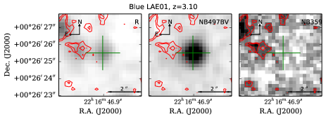
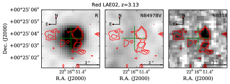
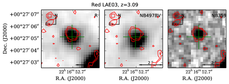
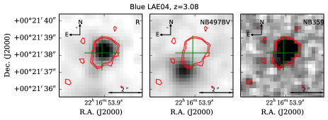
Figure 1: LAE LyC candidates. The green cross marks the location of the R band detection. The filter order is always R, NB497$-$BV (continuum-subtracted Ly$\alpha$), NB359 (LyC). The $2$ and $3\sigma$ contours trace the LyC detection in the NB359 band, and are overplotted in all other bands. For display purposes each filter has global contrast settings, so that direct brightness comparison between LAE objects is possible. For example LAE02 is very faint in Ly$\alpha$ relative to LAE01 or LAE03. The scale bar is 2″in all images. The color map is inverted.

2.1.2 Image quality and limiting magnitude

The PSF FWHM was measured in all filters by fitting a Moffat function to stars in the field. The number of stars varied from filter to filter but the final FWHM was always the median of $\gtrsim 1200$ stars. The B band PSF had FWHM$=0.78\arcsec\pm 0.12\arcsec$. For the V, R, i^′, z^′, NB359, and NB497 bands the measurements were $0.82\arcsec\pm 0.12\arcsec$, $1.06\arcsec\pm 0.12\arcsec$, $0.78\arcsec\pm 0.22\arcsec$, $0.77\arcsec\pm 0.18\arcsec$, $0.80\arcsec\pm 0.27\arcsec$, and $1.00\arcsec\pm 0.11\arcsec$, respectively. When performing analysis involving all seven filters, we therefore convolve all images to a common PSF of $\sim 1.00\arcsec$. However, since the PSF is not only better in the majority of filters but also fairly similar, we also separately analyze the unconvolved images in the B,V, i^′, z^′, and NB359 bands. Although there is scatter, there is no discernible systematic pattern in the spatial distribution of stellar FWHMs across the frames in any filter. The $3\sigma$ limiting magnitudes were obtained from $\sim 20000$ rectangular apertures with area equivalent to a $\diameter=1.2\arcsec$ circular aperture (difference $\sim 1\%$) on empty sky regions and measured to be B $=28.6^{m}$, V $=28.3^{m}$, R $=28.1^{m}$, i^′ $=27.8^{m}$, z^′ $=27.2^{m}$, NB359 $=27.4^{m}$, and NB497 $=27.7^{m}$ on $1.0\arcsec$ PSF convolved and Galactic extinction corrected frames.

All photometry has been corrected for Galactic extinction following Schlafly & Finkbeiner (2011), with individual $A_{V}$ values obtained for each object from the galactic Dust Reddening and Extinction calculator at the NASA/IPAC Infrared Science Archive. The individual extinction $A_{V}$ corrections in magnitudes are provided in the online catalog.

2.1.3 Images and Contours

In Figures 1 and 3 we present images of our LyC candidates in the reference R band, and the two other most informative bands, NB359 (LyC) and NB497 (Ly$\alpha$ for sources at $z\sim 3.09$). To highlight the Ly$\alpha$ emission we actually show NB497$-$BV, which subtracts the continuum making it easier to detect any offsets between Ly$\alpha$ and LyC. The BV image was constructed following $(2B+V)/3$ (Hayashino et al., 2004). Overplotted on all images are the $2$ and $3\sigma$ contours of the NB359 detection, and the position of the R detection is marked with a green cross.

2.2 HST data

For some targets Hubble Space Telescope (HST) Advanced Camera for Surveys (ACS) and/or Wide Field Camera 3 (WFC3) data is available from the archive in filters overlapping our observed wavelength range. We use this data only for visual analysis of the visible substructure since ground-based resolution precludes such insight. World coordinate system (WCS) inconsistencies in the HST images compared to our data were corrected beforehand with a full plate solution where possible. The LyC candidates with available HST data are summarized in Table 5, the images shown in Figure 17.

3 Sample selection

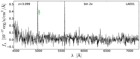
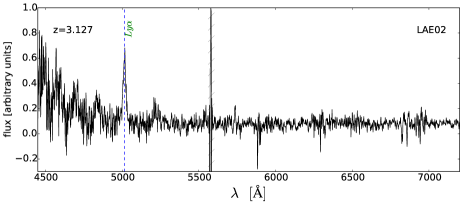
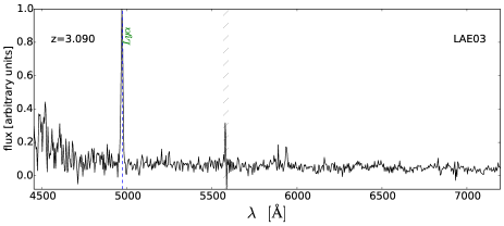
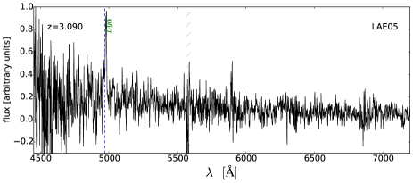
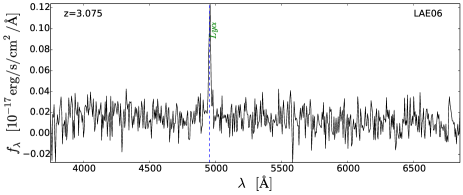
Figure 20: Spectra of the LyC candidates from FOCAS $2003$ (LAE01), FOCAS $2010$ (LAE02, LAE03, LAE05), VIMOS $2008$ (LAE06, LAE07, LAE08, LAE10, LAE14, LAE15, LBG02), and VIMOS $2006$ (LBG01, LBG03).

We found a total of $308$ galaxies ($136$ LBGs, $159$ LAEs, and $13$ AGN) in the SSA22 field, all with spectroscopically confirmed redshifts of $z\geq 3.06$. To qualify as a LyC candidate a source had to be detected at $\geq 3\sigma$ significance with $1.2\arcsec$ diameter aperture and it had to be within a radius $r=1.4\arcsec$ ($\sim 10$ kpc at $z\sim 3.1$) from the R band detection position. The obtained $30$ LyC candidates, listed in Table 1, contained five confirmed contaminants which we include in our contamination estimation (Sec. 3.1) but exclude from the all other analysis and figures. Excluding the confirmed contaminants the sample of LyC candidates consists of $7$ LBGs and $18$ LAEs. Suprime-Cam images are presented in Figures 1 (LAEs) and 3 (LBGs), and the accompanying spectra in Figure 20 in the appendix.

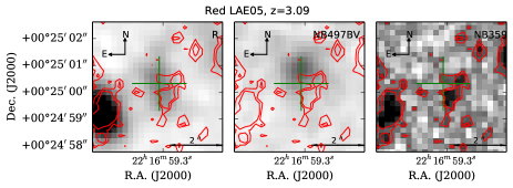
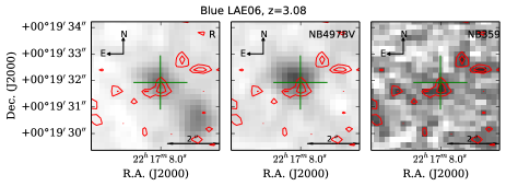
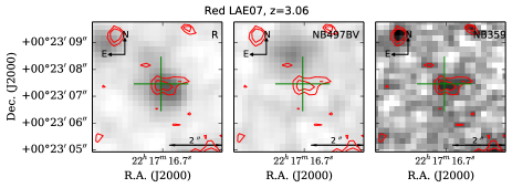
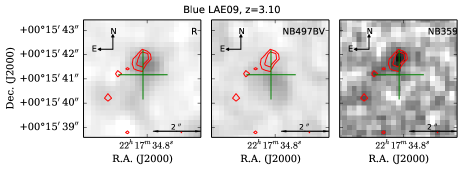
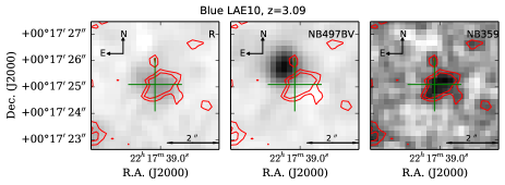
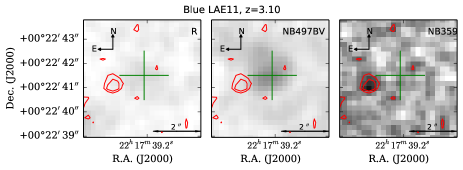
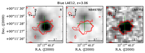
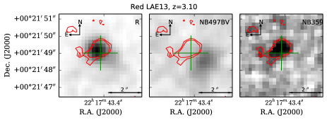
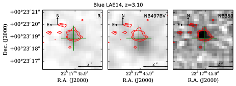
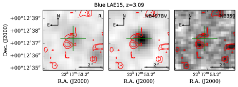
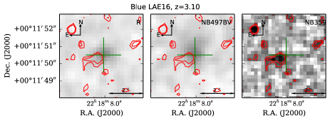
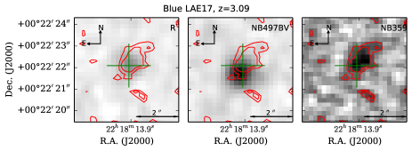
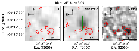
Figure 2: continued

SourceExtractor detections in the R band were considered to be the reference positions of the sources. For some targets the position of the LyC emission was offset from the reference position or from the position of the Ly$\alpha$ emission. Similar offsets have been found in previous studies (e.g., Iwata et al., 2009; Mostardi et al., 2013; Nestor et al., 2011, 2013). The reason we considered offset LyC-emitting objects to possibly be a part of the main galaxy at the reference position is because strongly star-forming galaxies are likely to have disturbed morphology with clumpy substructures spread throughout the galaxy. There are also arguments in the literature that dust and gas geometry plays a significant role in creating escape tunnels for both Ly$\alpha$ and LyC (e.g., Rauch et al., 2011), and consequently the LyC leakage would not be expected to be isotropic and may only be detectable from an individual star-forming region in the galaxy. In such a case, restricting ourselves to non-offset LyC candidates, as often done in the literature (e.g. Vanzella et al., 2010; Siana et al., 2015; Guaita et al., 2016), would cause an underestimation of the number density of LyC emitting galaxies and the cosmic average $f_{esc}$. However, our approach indeed allows for foreground contamination of the LyC candidates, and thus, we correct for contamination statistically in Sec 3.1.2. Note that these two approaches are both meaningful and complementary.

We have flagged $13$ out of $18$ LyC LAEs and $3$ out of $7$ LyC LBGs as possible but unconfirmed contaminants. Our reasoning and justification is summarized in Section A in the appendix, together with available HST images and spectra. The distribution of LyC offsets for the entire sample is shown in Figure 5, where NB359 traces LyC, NB497 traces Ly$\alpha$, and NB497-BV is the continuum subtracted Ly$\alpha$ emission.

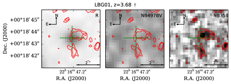
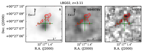
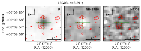
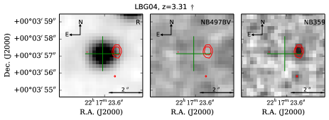
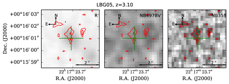
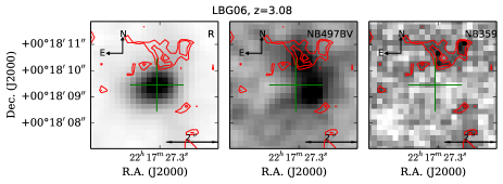
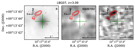
Figure 3: Same as in Fig. 1 but for the LBG LyC candidates. Note that for LBGs with redshifts outside the NB497 filter range ($3.06<z<3.13$) the NB497$-$BV image does not represent Ly$\alpha$ emission. These redshifts are marked with $\dagger$.

3.1 Contamination

The contamination rate in general would depend on the depth of the data, the spatial resolution, and the redshift (Siana et al., 2015). It was not possible to spectroscopically determine if there are any more foreground contaminants in our sample due to the lack of any convincing feature in their spectra. We therefore turn to statistical estimates.

3.1.1 False detection rate

We estimated the false detection rate by using a SourceExtractor catalog of detections obtained from a negative of the NB359 frame, crossmatched with the catalog of R band detections. The search radius for spurious detections was $1.4$″, as in the original detection procedure for LyC candidates. The false detection rate for sources above our detection limit is $1.9\%$, or $2.6$ false detections among $136$ LBGs, and $3.0$ false detections among $159$ LAEs. Additionally, we have checked the reliability of the detections in the NB359 image. We have confirmed that all LyC candidates are detected (at the $2\sigma$ level) separately in the two images comprising the final stacked NB359 image.

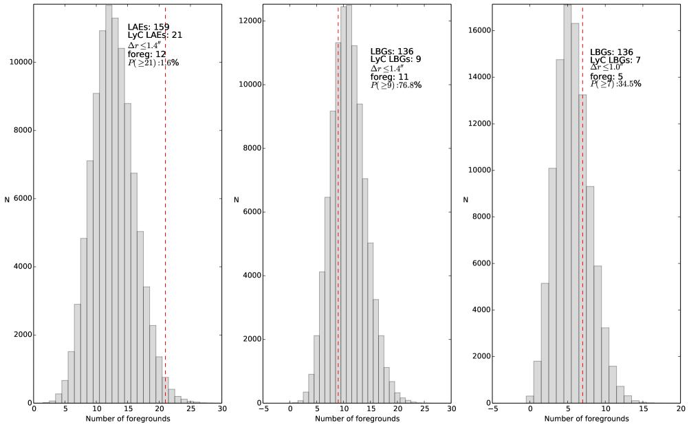
Figure 4: Expected number of contaminants from $100,000$ MC realizations for different $\Delta r$ offset measurements. The total number of objects in the current base sample, the total number of LyC candidates, the assumed offset $\Delta r$, the median number of contaminants in MC tests ’foreg’, and the probability $P$ that all LyC candidates are contaminants are indicated in the inset of each panel. The number of input objects in each simulation is marked by the dashed red line.

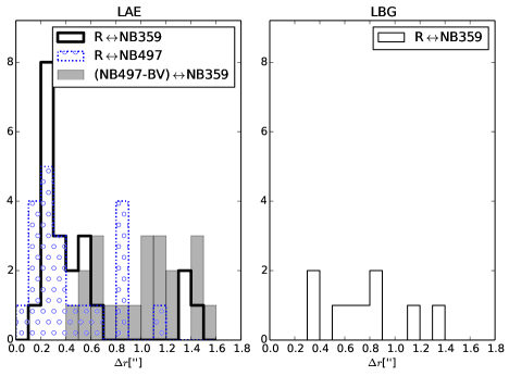
Figure 5: Offset distributions for LAEs and LBGs. For LAEs we have made use of the available multiwavelength data to investigate additional offset measurements.

3.1.2 Statistical contamination rate

We estimate the statistical probability of contamination in three different ways. Our primary procedure relies on the actual detections in the NB359 (LyC) image. The effect of possible spurious detections is therefore taken into account. This procedure assumes that foreground objects and our target LAEs and LBGs are not spatially correlated and is based on a Monte-Carlo (MC) simulation. In each MC realization we randomly place $N$ number of sample galaxies in the NB359 frame, where $N$ is $159$ for LAEs, and $136$ for LBGs. We search a circular area with a radius of $\Delta r$ around each randomly placed position for objects with detection significance $\geq 3\sigma$ in the SourceExtractor catalog. For each position if at least one object is detected the total number of contaminants for that realization is increased by one. This procedure is repeated $100,000$ times. The resulting distribution of expected number of contaminants for the $N=159$ LAEs and $\Delta r=1.4\arcsec$ is shown in the left panel of Figure 4. For LAEs the contaminant distribution shows that it is statistically unlikely for all $21$ LyC LAEs to be foreground contaminated. The median number of the contaminants is $12$ out of $21$. For $N=136$ LBGs and $\Delta r=1.4\arcsec$ the distribution is shown in the middle panel of Figure 4. The probability that there are at least $9$ foreground contaminants is $P(\geq 9)\sim 77\%$. All except two LyC LBG candidates have offsets lower than $1\arcsec$ (see Figure 5), so in the right panel of Figure 4 we show the expected number of contaminants for an assumed offset of $\Delta r\leq 1\arcsec$. The probability that all seven LyC LBGs are contaminated is $P(\geq 7)\sim 35\%$, still high, but significantly reduced.

We also investigated the possible effect of large scale structure variations on the results. To remove any large scale fluctuations in the spatial distribution of NB359 detections we performed the same MC simulation but this time assuming a uniform distribution of the NB359 detections, while preserving their total number. The expected number distribution of contaminants from this test did not show any significant differences, so in our case large scale fluctuations are not expected to alter the results.

We perform two additional tests. We adopt the same method as Vanzella et al. (2010), who used number counts from the ultradeep VIMOS U band imaging of the GOODS-South field (Nonino et al., 2009) to estimate the chance of foreground contamination of redshift $z\gtrsim 3$ galaxies. The magnitude range in our NB359 band is $24.0\leq AB\leq 27.0$. The corresponding U band surface number density of sources in our magnitude range is $\rho=248000$ deg^-2 according to Nonino et al. (2009). With our resolution of $1\arcsec$, the chance that an individual object is contaminated by a foreground galaxy is thus $P_{cont,obj}=6.0\%$. This is the Poisson probability to get one contaminant within a circular aperture with a radius of $1\arcsec$ under the expected number of $0.06$ according to the Nonino et al. (2009) number counts. The probability that at least $10$ out of $295$ objects are contaminated by foregrounds is very high, $P_{cont,10}\sim 98.5\%$. This is a binomial distribution probability assuming a success probability of $P_{cont,obj}$. The probability that all $30$ LyC candidates are foreground contaminants is negligible, $P_{cont,ALL}\sim 0.40\%$. Similarly, the probability for all $21$ LyC LAEs to be contaminants is $P_{cont,LAEs}\sim 0.06\%$. For $P_{cont,ALL}$ to go up to $\sim 50\%$ the U band number counts in Nonino et al. (2009) would have to be underestimated by a factor of $1.67$, or $67\%$. The number counts in the literature can vary, for example for the same magnitude range the number counts reported by Rovilos et al. (2009) differ by those of Nonino et al. (2009) by $10\%$. A $67\%$ uncertainty is therefore unlikely. This second contamination estimation is fully consistent with the results from the MC procedure based on our actual NB359 image.

As a final test, we have compared our primary MC procedure to the method presented in Nestor et al. (2013), which takes the individual offsets for each object into account but assumes a constant U band number density across the field of view. A test run of $1000$ MC realizations of the Nestor method with a search radius of $\Delta r=1.4$″ results in five (three) expected contaminants out of nine ($21$) LyC LBGs (LyC LAEs) using the offset $\Delta r=$R$\leftrightarrow$ LyC. Using the $\Delta r=$Ly$\alpha$$\leftrightarrow$ LyC offset for LAEs results in $15$ expected contaminants out of $21$ LyC LAEs. These results are qualitatively consistent with our method if we also assume constant number counts. As demonstrated they are highly dependent on which offset measurement one uses (e.g., $\Delta r=$R$\leftrightarrow$ LyC, $\Delta r=$R$\leftrightarrow$ Ly$\alpha$, or $\Delta r=$Ly$\alpha$$\leftrightarrow$ LyC, where the double arrow indicates the offset is measured between the corresponding two filters).

In conclusion, it is highly unlikely at a $98\%$ confidence level that all $21$ LyC LAEs are contaminants. The situation for the LyC LBGs is statistically much less convincing, however this group contains some of our most viable candidates, with no spatial offsets in LyC emission, and clean spectra with no mysterious emission lines.

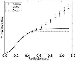
Figure 6: Example growth curve modeling, here for LAE06 in the i^′ band.

Table 2: Photometry of LyC candidates at the position of the R band detection. FWHM($\arcsec$) is measured from the reference R band. The omitted uncertainties for the R($1.2\arcsec$) column are $<0.1$ mag. Galactic extinction by Schlafly & Finkbeiner (2011) has been applied to all values. The $(f_{1500}/f_{900})$ column at the position of the R band is the observed total flux density ratio. Possible (but unconfirmed) contaminants are indicated with a ’^⋆’.

Red LAEs
ID	z	FWHM(″)	R	R($1.2\arcsec$)	NB359	NB359($1.2\arcsec$)	$(f_{1500}/f_{900})_{obs}$
LAE01⋆	$3.099$	$1.3$	$25.81\pm 0.04$	$26.79$
LAE02⋆	$3.127$	$1.4$	$23.53\pm 0.02$	$24.79$	$24.58\pm 0.06$	$26.56\pm 0.10$	$2.64\pm 0.16$
LAE03⋆	$3.090$	$1.1$	$24.41\pm 0.03$	$25.29$	$25.44\pm 0.08$	$26.32\pm 0.09$	$2.59\pm 0.20$
LAE05⋆	$3.088$	$1.4$	$25.26\pm 0.07$	$26.43$	$25.19\pm 0.11$	$26.85\pm 0.11$	$0.94\pm 0.11$
LAE07⋆	$3.065$	$1.3$	$25.19\pm 0.06$	$26.28$	$25.91\pm 0.10$	$26.83\pm 0.11$	$1.94\pm 0.20$
LAE08⋆	$3.080$	$1.4$	$24.84\pm 0.04$	$26.04$	$25.09\pm 0.09$	$26.49\pm 0.10$	$1.25\pm 0.12$
LAE13⋆	$3.097$	$1.1$	$24.93\pm 0.02$	$25.85$	$25.31\pm 0.09$	$26.27\pm 0.09$	$1.42\pm 0.11$
Blue LAEs
ID	z	FWHM(″)	R	R($1.2\arcsec$)	NB359	NB359($1.2\arcsec$)	$(f_{1500}/f_{900})_{obs}$
LAE04⋆	$3.085$	$1.0$	$24.74\pm 0.02$	$25.61$	$24.37\pm 0.08$	$25.52\pm 0.06$	$0.71\pm 0.06$
LAE06	$3.075$	$1.1$	$25.64\pm 0.05$	$26.53$	$25.45\pm 0.12$	$26.76\pm 0.11$	$0.85\pm 0.10$
LAE09⋆	$3.099$	$1.5$	$25.37\pm 0.05$	$26.73$	$25.63\pm 0.12$	$27.24\pm 0.13$	$1.27\pm 0.15$
LAE10⋆	$3.090$	$1.2$	$25.69\pm 0.07$	$26.72$	$25.34\pm 0.10$	$26.47\pm 0.09$	$0.72\pm 0.08$
LAE11⋆	$3.098$	$1.6$	$26.53\pm 0.08$	$27.78$	$25.89\pm 0.10$	$27.93\pm 0.18$	$0.56\pm 0.07$
LAE12⋆	$3.065$	$1.7$	$23.96\pm 0.05$	$25.53$	$24.40\pm 0.09$	$25.73\pm 0.07$	$1.49\pm 0.14$
LAE14	$3.095$	$1.1$	$25.78\pm 0.07$	$26.73$	$25.26\pm 0.10$	$26.39\pm 0.09$	$0.62\pm 0.07$
LAE15	$3.094$	$1.3$	$25.67\pm 0.08$	$26.81$	$25.35\pm 0.12$	$26.82\pm 0.11$	$0.75\pm 0.10$
LAE16	$3.096$	$0.8$	$26.15\pm 0.04$	$26.93$	$25.74\pm 0.14$	$27.09\pm 0.13$	$0.69\pm 0.09$
LAE17	$3.089$	$0.8$	$26.19\pm 0.04$	$26.78$	$25.27\pm 0.10$	$26.32\pm 0.09$	$0.43\pm 0.04$
LAE18⋆	$3.087$	$1.1$	$26.45\pm 0.06$	$27.22$	$25.51\pm 0.17$	$28.22\pm 0.21$	$0.42\pm 0.07$
LBGs
ID	z	FWHM(″)	R	R($1.2\arcsec$)	NB359	NB359($1.2\arcsec$)	$(f_{1500}/f_{900})_{obs}$
LBG01	$3.680$	$0.9$	$24.66\pm 0.02$	$25.53$	$25.49\pm 0.12$	$26.76\pm 0.11$	$2.15\pm 0.25$
LBG02	$3.113$	$1.2$	$24.31\pm 0.02$	$25.46$	$26.05\pm 0.22$	$27.18\pm 0.13$	$4.98\pm 1.00$
LBG03	$3.287$	$0.8$	$24.69\pm 0.02$	$25.44$	$25.18\pm 0.11$	$27.22\pm 0.13$	$1.58\pm 0.17$
LBG04	$3.311$	$1.0$	$23.44\pm 0.01$	$24.30$	$26.64\pm 0.27$	$27.83\pm 0.18$	$19.01\pm 4.72$
LBG05⋆	$3.102$	$1.1$	$25.05\pm 0.05$	$26.11$	$25.87\pm 0.14$	$27.17\pm 0.13$	$2.13\pm 0.28$
LBG06⋆	$3.080$	$1.4$	$23.44\pm 0.01$	$24.61$	$24.54\pm 0.30$	$28.83\pm 0.27$	$2.76\pm 0.76$
LBG07⋆	$3.094$	$1.4$	$24.25\pm 0.02$	$25.43$	$25.63\pm 0.34$	$28.07\pm 0.20$	$3.57\pm 1.12$

4 Suprime-Cam Photometry

Two types of BVRi^′z^′, NB497, and NB359 measurements are used in the analysis and made available in the online catalog, along with FWHM, Galactic extinction correction, and LyC offset. One magnitude measurement represents the total magnitude of the source with individual aperture size, and one with a fixed $\diameter=1.2\arcsec$ aperture size for all sources. UV and LyC photometry are summarized in Table 2. Additionally, in Table 3 we list the V$-$i^′ and NB359$-$R colors for each object, along with probability of contamination $P$ based on measured offsets between the NB359 detection and either NB497$-$BV (for LAEs) and R band (for LBGs). For the calculation of $P$ we obtain the surface number density $\rho=177327$ deg^-2 from the NB359 image.

The existence of spatial offsets implies that for some LyC candidates the $\diameter=1.2\arcsec$ aperture photometry at the R band position will not represent the total strength of the LyC emission. Therefore the online catalog also provides the $\diameter=1.2\arcsec$ aperture photometry at the position of the NB359 detection. This fixed aperture is not large enough to measure the total magnitude in every case but it could highlight any intrinsic differences between the sources on equal spatial scales (for objects at the same redshift). For the position of the R band we perform both types of photometry in all filters, while for the position of the NB359 band we only obtain the $\diameter=1.2\arcsec$ aperture photometry.

To measure the total magnitude of a given source we first construct its growth curve with the IRAF PHOT task and a range of apertures. Then we model a synthetic object with the same axis ratio as the original object, same total magnitude and Gaussian radial profile, convolve it with the seeing of the frame, and measure its growth curve. We do this for a range of total magnitudes and FWHMs, centered at the preliminary results obtained through SExtractor photometry, which also provides the axis ratio of the synthesized object. For each galaxy in the sample all model growth curves are examined visually and an individual decision on the cutoff radius is made, resulting in one cutoff radius per galaxy. The growth curve which gives the smallest $\chi^{2}$ compared to the original growth curve is chosen as the best model for that object and is used to provide its asymptotic total magnitude. In an attempt to accommodate differences in object shapes this procedure is performed for two initial models, one with a synthetic object following a Gaussian profile, convolved with a Gaussian PSF, and the other with a synthetic object following a Gaussian profile, convolved with a Moffat PSF. One model is therefore a pure Gaussian even after convolution, while the other is a Gaussian/Moffat hybrid. For brevity we refer to the latter simply as the Moffat model. For each object we therefore have two best model growth curves. When these two show significant differences in their asymptotic magnitudes we visually examine which growth curve best follows the original growth curve and choose the appropriate asymptotic total magnitude for that object. The concept is illustrated in Figure 6. The same procedure gives the best FWHMs for each object. Here we note that the resolution is such that the measured FWHM is unreliable since it is often comparable to those of the point sources. We therefore cannot use the best-fit FWHM as a measure of the object size in the absence of atmospheric distortion.

4.1 Uncertainties

The photometric uncertainties for the fixed $\diameter=1.2\arcsec$ aperture are obtained from the output of IRAF PHOT, with some modifications. Initial tries showed unsatisfactory estimation of the sky background value with IRAF PHOT for a number of targets due to the far wings of bright saturated stars in the sky annuli. The calculated mode of the values inside the sky annulus did not take into account the cases where the sky histogram had several nearby peaks with similar amplitudes. To estimate the background more reliably we instead measured for each target the weighted average of all data points within $\pm 5\%$ of the mode in the sky annulus histogram. This constant sky value was then used in IRAF PHOT to obtain new error measurements. To correct for the effect that a constant sky value has on the IRAF PHOT errors, we additionally corrected these with the uncertainty in the sky level (Section 2.1.2), which was assumed constant throughout the frame. These are the errors listed in our catalog for fixed $\diameter=1.2\arcsec$ aperture photometry.

The uncertainties in the asymptotic total magnitudes (“model mag”) are obtained by an MC simulation with 1000 runs per object per model per filter, where each realization perturbs each data point of the original growth curve by a random value drawn from a $1\sigma$ normal distribution, where $\sigma$ is the error of the current data point. This gives a range of model growth curves which best fit each perturbed realization. The asymptotic magnitude uncertainty for a given target, model, and filter is then the standard deviation of the $1000$ asymptotic magnitudes from the MC simulation. The MC uncertainties for Gaussian models are on average larger than those for the Moffat models by $\lesssim 10\%$. For derived quantities, such as the flux density ratios and the equivalent width, the uncertainties were obtained through error propagation.

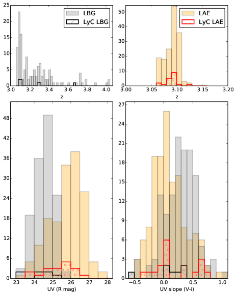
Figure 7: Rest-frame UV magnitude (R band, left) and the distribution of the measured UV slopes (V$-$i^′, right) for all LAEs (orange bars) and all LBGs (gray bars) in the sample. LyC LAE (dotted bars) and LyC LBG (hatched bars) candidates are also shown. AGN and confirmed foreground contaminants are not included. All measurements are of the total magnitudes. The redshift distributions of the full LAE and LBG samples, as well as the LyC subsamples, are shown in the top panels.

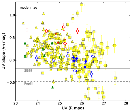
Figure 8: Rest frame UV slope versus non-ionizing total UV magnitude at the position of the R band for the full sample. The control sample of non-LyC are shown in yellow markers (triangle - LBG, square - LAE). Red and blue LyC LAEs are colored accordingly, LyC LBGs with green triangles. Possible but unconfirmed LyC contaminants are indicated with open markers of the corresponding shape and color. Bluest V$-$i^′ model predictions from a SB 99 and a Pop III model are plotted with solid, respectively dashed lines.

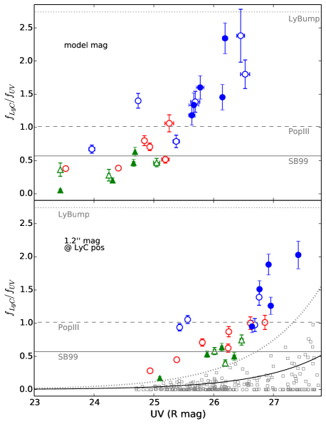
Figure 9: Observed flux density ratios for total brightness at the R position (upper panel) and $1.2\arcsec$ fixed aperture measurements at the NB359 position (lower panel) for the LyC candidates. The horizontal lines and the marker legend are the same as in Fig. 8, with an added line for the LyBump Pop III model (see Sec. 5.2 for details). For convenience the $1\sigma$ (black curve) and $3\sigma$ (gray dotted curve) detection limits from $1.2\arcsec$ apertures in the NB359 (LyC) band are also shown. LAE11 and LAE18 are omitted from the lower panel because they are too faint in $1.2\arcsec$ R band photometry at the position of the NB359 band. The open gray squares are the LyC non-detections from both the LAE and LBG base samples.

4.2 Variability

Vanzella et al. (2015) suggest that low luminosity AGNs hidden in star forming galaxies could be responsible for the detected LyC emission from these galaxies. We performed a brightness variability test on all objects in our samples to detect potential AGNs. None of the LyC candidates show any variability in brightness over the span of 6 years, however it is still possible that low luminosity AGNs could be present and either be non-variable, vary on amplitudes below our detection level, or vary with a shorter time-scale than our sampling ($\sim 1$ year). The individual light curves are shown in Figure 23 in the appendix.

5 Properties of LyC sources

With respect to the UV continuum on average the LBGs in the sample are brighter than the LAEs, which is expected since the strong Ly$\alpha$ emission line deepens the detection limit in spectroscopically confirmed samples of galaxies. The distribution of total rest-frame UV brightness for the sample is shown in Figure 7, where we also show the distribution of V$-$i^′ colors and redshifts from Table 3. We use V$-$i^′ color (approximately flux density ratio between 133nm and 188nm for a galaxy at $z=3.1$) to investigate rest-frame UV slope. Despite the difference in brightness ranges, the color distribution has an overlapping range for LAEs and LBGs, with the LBGs being on average redder than the LAEs, which is consistent with the literature (e.g. Gronwall et al., 2007) and reflects the different nature of these types of galaxies. Note that the fraction of LyC LBG candidates seems to be relatively small in the proto-cluster. A comparatively similar amount of LyC LBG candidates are found at higher redshifts, unassociated with the proto-custer. The LyC LAEs show a broad range of colors. To highlight any effects such color differences may have on the properties of these galaxies, we divide them into red LAE (V$-$i^′$>0.2$) and blue LAE (V$-$i^′$\lesssim 0.2$). Note that this separation is quite arbitrary, we simply aim to distinguish between the very red and very blue LAEs. We feel such a separation may be meaningful because the number of LyC candidates is overrepresented among the extremely red LAEs. The two photometry tables (Tab. 2 and 3) show the blue/red labels for the LAE sample.

Table 3: LyC candidates V$-$i^′ and NB359$-$R colors at the position of the R band detection. Redshift $z$ and LyC offset $\Delta r$ (″) are indicated for convenience. The individual probability for contamination $P$, indicated in per cent, is calculated as $P=\rho\pi\Delta r^{2}$, where $\rho=1.77327e5$ deg^-2 is the surface number density we obtain from the NB359 image.

ID	z	V$-$i′	NB359$-$R	$\Delta r^{\dagger}$	$P[\%]$
Red LAE viable candidates
-
Red LAE possible contaminants
LAE01	$3.099$	$0.65\pm 0.06$		$1.4$	$8.4$
LAE02	$3.127$	$0.67\pm 0.02$	$1.05\pm 0.07$	$0.9$	$3.5$
LAE03	$3.090$	$0.65\pm 0.04$	$1.03\pm 0.08$	$0.5$	$1.1$
LAE05	$3.088$	$0.38\pm 0.09$	$-0.06\pm 0.13$	$1.1$	$5.2$
LAE07	$3.065$	$0.74\pm 0.08$	$0.72\pm 0.11$	$1.3$	$7.3$
LAE08	$3.080$	$0.55\pm 0.05$	$0.24\pm 0.10$	$1.5$	$9.7$
LAE13	$3.097$	$0.35\pm 0.05$	$0.38\pm 0.09$	$1.2$	$6.2$
Blue LAE viable candidates
LAE06	$3.075$	$0.06\pm 0.06$	$-0.18\pm 0.13$	$0.4$	$0.7$
LAE14	$3.095$	$0.04\pm 0.07$	$-0.51\pm 0.12$	$0.8$	$2.8$
LAE15	$3.094$	$-0.01\pm 0.08$	$-0.32\pm 0.15$	$0.5$	$1.1$
LAE16	$3.096$	$-0.15\pm 0.08$	$-0.41\pm 0.14$	$0.7$	$2.1$
LAE17	$3.089$	$-0.02\pm 0.05$	$-0.92\pm 0.11$	$0.7$	$2.1$
Blue LAE possible contaminants
LAE04	$3.085$	$0.01\pm 0.04$	$-0.37\pm 0.09$	$1.4$	$8.4$
LAE09	$3.099$	$0.10\pm 0.08$	$0.26\pm 0.13$	$0.8$	$2.8$
LAE10	$3.090$	$-0.23\pm 0.09$	$-0.35\pm 0.12$	$1.0$	$4.3$
LAE11	$3.098$	$0.09\pm 0.11$	$-0.64\pm 0.13$	$1.2$	$6.2$
LAE12	$3.065$	$0.06\pm 0.06$	$0.43\pm 0.10$	$1.1$	$5.2$
LAE18	$3.087$	$-0.31\pm 0.07$	$-0.94\pm 0.18$	$1.2$	$6.2$
LBG viable candidates
LBG01	$3.680$	$0.39\pm 0.04$	$0.83\pm 0.12$	$0.5$	$1.1$
LBG02	$3.113$	$0.11\pm 0.02$	$1.74\pm 0.22$	$0.9$	$3.5$
LBG03	$3.287$	$-0.60\pm 0.02$	$0.50\pm 0.12$	$0.8$	$2.8$
LBG04	$3.311$	$0.38\pm 0.02$	$3.20\pm 0.27$	$0.8$	$2.8$
LBG possible contaminants
LBG05	$3.102$	$0.08\pm 0.07$	$0.82\pm 0.15$	$0.3$	$0.4$
LBG06	$3.080$	$0.09\pm 0.02$	$1.10\pm 0.30$	$1.1$	$5.2$
LBG07	$3.094$	$0.24\pm 0.02$	$1.38\pm 0.34$	$1.3$	$7.3$

$\dagger$ For LAEs, $\Delta r=($NB497$-$BV$)\leftrightarrow$NB359. For LBGs $\Delta r=$R$\leftrightarrow$NB359. The double arrow indicates the offset is measured between the corresponding filters.

5.1 The UV slope

In Figure 8 we show the color-magnitude distribution of the LyC candidates and the control sample using modeled asymptotic growth curve magnitude measurements from Tables 2 and 3. The red LyC LAEs are on average brighter than the blue LyC LAEs. Note that our morphology/spectrum analysis in Sec. 3 flagged all red LyC LAEs as possible but unconfirmed contaminants independently of their extreme red colors. The LyC candidates in general occupy the same parameter space as the non-LyC sample and in both groups there are some galaxies that show extremely blue UV slopes independent of magnitude. These violate the model predictions from Starburst 99 (Leitherer et al., 1999, SB 99) shown as a gray horizontal line, and also those from a Population III model (Schaerer, 2003, Pop III), shown as a gray dashed line. Both models are for zero age, with mass range $1$-$100M_{\sun}$, a Salpeter IMF ($\alpha=2.35$), no nebular emission, and either zero or low ($Z=0.0004$) metallicity. These are the bluest stellar evolutionary models for this IMF since increased age and metalicity, as well as accounting for nebular emission, will make the colors redder. Although the larger uncertainty at fainter magnitudes affects the colors, fainter galaxies appear to have bluer UV slopes. These galaxies are dominated by LAEs because of the faint limit detection bias favoring LAEs over LBGs.

5.2 Ionizing to non-ionizing flux density ratios

Figure 9 shows the flux density ratios of the ionizing to non-ionizing radiation as it varies with UV brightness using data from Table 2 and our online catalog. For both axes we use the R band to sample the non-ionizing radiation. It is immediately obvious that some LyC candidates, mostly the blue LAEs, have extremely high flux density ratios. While these galaxies are among the faintest, their LyC detections are well above the $3\sigma$ limit. The extreme ratios are preserved when measuring the flux at the offset position of the NB359 (LyC) band (bottom panel). The possible contaminants LAE11 and LAE18 are omitted from the bottom panel because they are very faint already at the R band position and are well below the detection limit in R at the position of the NB359 band.

As Figure 9 demonstrates, many of the observed LAE flux density ratios imply at least a flat spectrum with no Lyman Break, i.e. a ratio of $f_{LyC}/f_{UV}=1$ (NB359$-$R $=0$) which is inconsistent with current “standard” population synthesis models, as indicated by the SB99 line in the figure. The presence of IGM is expected to further decrease the observed flux density ratio.

There are, however, physically consistent models which predict higher flux density ratios than the standard models, such as the so-called Lyman limit ’bump’ model (Inoue, 2010). The model proposes that, instead of being completely absorbed, nebular LyC can escape through matter-bound nebulae along the same paths as stellar LyC. This nebular LyC contribution would compensate for the Lyman break by significantly contributing to the flux bluewards of the Lyman limit, causing the so-called ’bump’ and making the NB359$-$R much bluer than the “standard” models. The bluest NB359$-$R color prediction from this model is shown with a dotted line, for PopIII with a high mass range (50-500 $M_{\sun}$).

The existence of PopIII stars at $z\sim 2\mbox{-}3$ has been suggested by several theoretical works in the literature (e.g. Tornatore et al., 2007; Johnson, 2010), and pristine gas clouds in the IGM have already been found at $z\sim 3$ (e.g. Fumagalli et al., 2011) and Inoue et al. (2011) present a two component model which offers an explanation for the co-existence of PopIII stars and dust. In addition, there are other scenarios resulting in an effectively top-heavy IMF, which would contribute to a boost of the observed $f_{LyC}/f_{UV}$. Namely, runaway massive stars (Conroy & Kratter, 2012), and stochasticity in the IMF sampling (Forero-Romero & Dijkstra, 2013). The most massive stars from these scenarios, as well as the massive binary model, BPASS (Eldridge & Stanway, 2009), can give intrinsic $f_{LyC}/f_{UV}\sim 1$. This, in combination with the Lyman Bump mechanism, may help explain our observations.

Many of the LyC LAEs with flux density ratios $f_{LyC}/f_{UV}\gtrsim 1$ have small to insignificant spatial offsets, and were therefore not flagged as possible contaminants. We have shown in Sec. 3.1.2 that it is statistically highly unlikely for the full LyC LAE sample to be foreground contaminants: the cumulative probability to have $21$ or more contaminants is $1.6\%$, with a probability of $1\%$ to have exactly $21$ contaminants. Our observations are one single trial. We find no compelling reason to assume that in one single trial we have managed to observe an event which has $1\%$ probability of realization.

Consider further that even if all LyC LAE candidates with $f_{LyC}/f_{UV}\gtrsim 1$ are assumed to be foreground contaminants, this would not automatically explain their observed flux density ratios. Most of these objects have $1.5\lesssim f_{LyC}/f_{UV}\lesssim 2$. As a reminder, LyC is measured in the NB359 band with effective wavelength $\lambda_{eff}=359$ nm, and UV in the R band with $\lambda_{eff}=650$ nm. These objects therefore have $f_{\nu}\propto\nu^{0.7}$ to $f_{\nu}\propto\nu^{1.2}$, respectively. The corresponding UV slope range is $-2.7\lesssim\beta_{UV}\lesssim-3.2$. The average $\beta_{UV}$ for galaxies at $1\leq z<3$ is $\beta_{UV}=-1.5$ (e.g Bouwens et al., 2009; Kurczynski et al., 2014). Even if such extreme foreground objects exist, they would be very rare, further decreasing the probability that all of them are foreground contaminants.

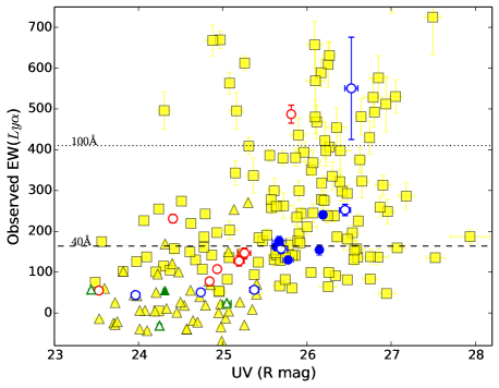
Figure 10: $EW($Ly$\alpha$$)$ vs. total UV magnitude. Rest-frame $EW($Ly$\alpha$$)$ for $z=3.1$ indicated with dashed/dotted lines for convenience. Only objects with redshift $3.06\leq z\leq 3.13$ are shown.

5.3 Observed Ly$\alpha$ Equivalent width

The NB497 band measures the Ly$\alpha$ line for galaxies in the redshift range $3.06<z<3.13$. Matsuda et al. (2009) derive a conversion formula for the observed equivalent width using the same NB497 band and a so-called BV image (BV$=(2$B$+$V$)/3$) with the same effective wavelength as the NB497 band:

$$EW(Ly_{\alpha})=\frac{(887+936)\times 77\times(10^{0.4(BV-NB497)}-1)}{(887+936)-0.6\times 77\times 10^{0.4(BV-NB497)}}$$

where $887$ Å, $936$ Å, and $77$ Å are the FWHMs of the B, V, and NB497 respectively. Using their formula in Figure 10 we show the observed $EW($Ly$\alpha$$)$ for objects associated with the proto-cluster. The redshift constraint imposed by the Ly$\alpha$ filter limits the non-LyC LBG sample to $46$ galaxies, and the non-LyC LAEs to $132$. Similar to previous results in the literature (e.g., Shapley et al., 2003; Ando et al., 2006), we find a statistically significant correlation at the $9\sigma$ level between decreasing galaxy brightness and increasing Ly$\alpha$ emission strength using both Spearman’s $\rho$ and Kendall’s $\tau$, which are $0.59$ and $0.41$, respectively. Nestor et al. (2011) find that LAE galaxies with LyC detection tend to have lower $EW($Ly$\alpha$$)$ than non-LyC LAE. In our sample of non-LyC LAEs the average is $\left<EW(Ly\alpha)\right>\sim 279\pm 16$Å, where the uncertainty is the standard error. For LyC LAEs it is $\left<EW(Ly\alpha)\right>\sim 178\pm 33$Å, which is significantly lower than the general population at a $>99\%$ confidence level, although the sample scatter is large. For the LBGs it is difficult to draw conclusions because there are only four LyC LBG candidates within the redshift range of the Ly$\alpha$ filter (Fig. 10). However small the sample, we can note that contrary to the literature, the average ($\sim 26$Å), weighted average ($\sim 34$Å, the individual uncertainty of each data point was used as weight), and median ($\sim 40$Å) $EW($Ly$\alpha$$)$ for these four LyC LBGs are consistent with or larger than those of the full LBG sample ($EW($Ly$\alpha$$)$$~{}\sim 34$Å, $~{}\sim 2$Å, $~{}\sim 19$Å). We cannot confirm or refute the claim that galaxies with LyC detection tend to have lower Ly$\alpha$ based on this investigation. However, even if true, this does not preclude the possibility of a positive LyC/Ly$\alpha$ correlation among the subgroup of galaxies with LyC emission.

5.4 Ly$\alpha$ vs LyC

The mechanisms that allows Ly$\alpha$ to escape from the confines of a galaxy are likely to also fascilitate the escape of LyC, especially if the main reason behind a successful escape is the geometry of the dust and gas distribution in the galaxy, and the presence of possible tunnels of low dust and gas density through which both Ly$\alpha$ and LyC can escape (Rauch et al., 2011). On the other hand, a simplified view of the post-production fate of ionizing radiation states that if most of the ionizing photons produce Ly$\alpha$ then the amount of LyC will be significantly decreased, if not zero. The intrinsic Ly$\alpha$ or LyC cannot be measured but it is nonetheless interesting to examine the observed Ly$\alpha$ and observed LyC for any possible correlations. There is a lot of scatter in Figure 11, in part surely due to the $EW($Ly$\alpha$$)$ conversion formula, and a statistically significant correlation cannot be inferred from e.g. Spearman’s $\rho=0.67$ or Kendall’s $\tau=0.5$ because the number of available data points is too small. Taken at face value, the figure would suggest that with decreasing $EW($Ly$\alpha$$)$ the flux density ratio also decreases and the most extreme $f_{LyC}/f_{UV}$ objects have significant $EW($Ly$\alpha$$)$. On the one hand this seeming correlation may be secondary, a product from the correlations between flux density ratio and luminosity in Figure 9, and $EW($Ly$\alpha$$)$ and luminosity in Figure 10. On the other hand, such a correlation would be consistent with the idea that both a Ly$\alpha$ and a LyC photon benefit from the same environmental conditions to escape. This is further supported by the fact that on average LAEs, which have a stronger Ly$\alpha$ emission, show a LyC emission greater than that of LBGs, as Figure 11 clearly indicates. Another possible explanation for this correlation may be a selection bias of the Lyman Break method which preferentially rejects galaxies with small amount of IGM attenuation and strong LyC emission (Cooke et al., 2014). Either way, we cannot reject the null hypothesis that $f_{LyC}/f_{UV}$ and $EW($Ly$\alpha$$)$ in Figure 11 are statistically independent with any confidence level worth mentioning.

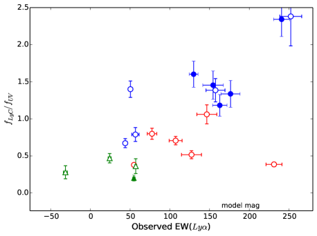
Figure 11: LyC versus Ly$\alpha$ equivalent width. LAE11 is omitted because it is too faint in B, V for reliable conversion to $EW($Ly$\alpha$$)$. Spearman’s correlation coefficient $\rho$ is $0.67$, and Kendall’s $\tau=0.5$, however the sample size is too small to infer a statistically significant correlation. If the correlation is real it suggests that with decreasing $EW($Ly$\alpha$$)$ the flux density ratio also decreases. Marker legend is the same as in Fig. 8.

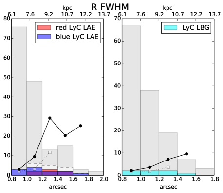
Figure 12: Distribution for FWHMs for all LAEs (left panel, gray bars) and all LBGs (right panel, gray bars). The dashed histogram in the left panel is all LyC LAE. The black connected circles are the ratio of LyC to non-LyC galaxies plotted on arbitrary horizontal scales in the corresponding bin (bin size 0.2″). In both panels the square markers with dotted connecting line are the same ratio but excluding the possible (but unconfirmed) contaminants.

5.5 Indications of mergers

We have measured the FWHMs of the LyC candidates as described in Sec. 4. In all filters there is a trend for the “large” galaxies to be more often also LyC leakers compared to the smaller galaxies. We show this for the R band in Figure 12. This is especially clear for LBGs but the trend is also there for LAEs. The Point Spread Function (PSF) of the images is $\sim 1\arcsec$ and consequently any FWHM which measures $\lesssim 1\arcsec$ simply indicates that we cannot resolve that object. Equally important is the fact that large FWHM does not indicate greater mass of the galaxy. Instead the large FWHMs come from the presence of offset substructures. Such substructures could indicate the infall/accretion of a minor object. For LBGs in the SSA22 proto-cluster a high merger fraction compared to field LBGs was recently found by Hine et al. (2016). We interpret the increased number of LyC candidates among the objects with large FWHMs as an indication that infall/accretion provides the necessary disturbance of the otherwise regular distribution of dust and gas in the galaxy, perhaps creating tunnels with low dust and gas density through which LyC escapes.

The probability for foreground contamination increases with offset between the LyC and UV positions (Vanzella et al., 2010). If large $f_{LyC}/f_{UV}$ ratios were due to foreground contaminants one may then expect large offsets for those objects as well. In Figure 13 we do not see such a trend.

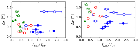
Figure 13: Flux density ratio versus the offset $\Delta r$, measured between R and NB359 (left panel), and between $($NB497$-$BV$)$ and NB359 (right panel). Marker legend is the same as in Fig. 8.

5.6 $\left<f_{LyC}/f_{UV}\right>_{obs}$ from stacking

We estimate the average flux density ratio from stacking. We exclude the confirmed contaminants from this analysis, however since our candidate sample may contain foreground contaminants we use a MC method with 100 realizations to obtain statistically corrected averages. All measurements are from $\diameter=1.2\arcsec$ apertures and corrected for Galactic extinction. First, for all galaxies in the sample we make $10\arcsec\times 10\arcsec$ cutouts from the NB359 image. For each object we normalize the cutout by the corresponding R band flux. In each MC realization the number of contaminants $n_{cont}$ is randomly drawn from the probability mass function we obtained in Section 3.1.2, shown in Figure 4. When stacking all LAEs (LBGs) a number of $N+n$ images are stacked, where $N=138$ ($N=127$) for LAE (LBG) non-detections in the NB359 filter, and $n$ is the remaining number of LyC candidates in that run, $n=18-n_{cont}$ ($n=7-n_{cont}$) for LAEs (LBGs). Occasionally the number of contaminants $n_{cont}$ is greater than the number of candidates, and we set $n=0$ so that only $N$ images are stacked in that MC run. The uncertainty in the resulting averages is estimated in each MC run for each object by randomly placing $100$ apertures on empty sky, normalizing each one by the object’s R band flux, and measuring the standard deviation of the aperture photometries at the 100 sky positions. As a sanity check of the uncertainty estimation we directly measured $\sigma$ from the final stacked images by placing a few apertures away from the central region and obtaining the standard deviation of the photometries. Although the available area is small, and the number of apertures therefore limited, these measurements are consistent with our MC estimation of the uncertainties.

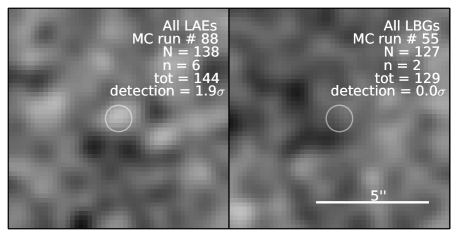
Figure 14: Average stacks of $10\arcsec\times 10\arcsec$ cutouts of NB359$-$R from example MC runs for all (LyC and non-LyC) LAEs and LBGs. $N$ is the number of non-detections in NB359 objects, $n$ is the number of LyC candidates for that MC run, and the MC run number is the realization identifier. The aperture is indicated with a circle. The contrast levels are set to $\pm 5\sigma$.

Figure 14 shows random MC runs for the stacks of all LAEs and LBGs. These example runs show a marginal detection of $1.9\sigma$ for the stack of all LAEs (left panel), and a non-detection for the stack of all LBGs (right panel). Note that even if there is a detection for a stack from a single MC realization, we obtain the average flux density ratio of all MC realizations and the final result may therefore be a non-detection.

Table 4: The average observed $3\sigma$ upper limits on $\left<f_{LyC}/f_{UV}\right>_{obs}$ from stacking all LAEs and all LBGs. The observed $\left<\textit{V}-\textit{i}^{\prime}\right>_{obs}$ is used to estimate the dust attenuation by comparing to model $(\textit{V}-\textit{i}^{\prime})_{i}$ predictions from SB99, with 100Myr. The relative and absolute escape fractions are shown for median IGM attenuation $\tau_{IGM}^{med}=0.74^{m}$. $(\textit{NB359}-\textit{R})_{i}$ is the intrinsic color. The average dust attenuation $\left<A_{UV}\right>$ is given for completion. The effect of foreground contamination is statistically corrected; see text for details.

stack	$\left<f_{LyC}/f_{UV}\right>_{obs}$	$\left<\textit{V}-\textit{i}^{\prime}\right>_{obs}$	$(\textit{NB359}-\textit{R})_{i}$	$(\textit{V}-\textit{i}^{\prime})_{i}$	$f_{esc}^{rel}$	$\left<A_{UV}\right>$	$f_{esc}$
LAEs	$<0.077$	$0.127$	$1.57$	$-0.19$	$<0.685$	$1.67$	$<0.147$
LBGs	$<0.020$	$0.350$	$1.57$	$-0.19$	$<0.181$	$2.80$	$<0.014$

Table 4 summarizes the results in terms of the average flux density ratios of $100$ such MC realizations. Since we have no $>3\sigma$ detection, we present $3\sigma$ upper limits instead. Nestor et al. (2013) obtain an observed emsemble average of $f_{LyC}/f_{UV}$ of $0.086\pm 0.036$ for LAEs and $0.017\pm 0.011$ for LBGs in the SSA22 field with a smaller areal coverage of $42$ arcmin². These are consistent with our $3\sigma$ limits of $<0.077$ for LAEs and $<0.020$ for LBGs. Our results are also consistent with Mostardi et al. (2013), who find an emsemble average of $0.060\pm 0.029$ for LAEs and $0.0043\pm 0.0024$ for LBGs in the proto-cluster HS1549+1933 at a comparable redshift of $z=2.85$. In fact, our upper limits are similarly consistent with all previous results in the literature, e.g. Vanzella et al. (2010, $z=3.6$ LBGs, $f_{LyC}/f_{UV}<0.002$), Boutsia et al. (2011, $z=3.3$ LBGs, $f_{LyC}/f_{UV}<0.013$), Grazian et al. (2016, $z=3.3$ LBGs, $f_{LyC}/f_{UV}<0.006$), Guaita et al. (2016, $z=3.4$ LBGs, $f_{LyC}/f_{UV}<0.026$), Smith et al. (2016, $z=3.5$ LBGs, $f_{LyC}/f_{UV}=4.66\cdot 10^{-3}\pm 1.20\cdot 10^{-3}$). We also tested stacking only non-detections in LyC but the result remained a non-detection, suggesting a possible bimodality of the LyC escape.

5.7 Escape fraction estimation

The escape fraction of LyC is defined as:

$$f_{esc}=\frac{L_{LyC,out}}{L_{LyC,int}}=\frac{\left(f_{LyC}/f_{UV}\right)_{obs}}{\left(f_{LyC}/f_{UV}\right)_{int}}10^{-0.4A_{UV}}e^{\tau_{IGM,LyC}}$$

where $\left(f_{LyC}/f_{UV}\right)_{int}$ is the intrinsic flux density ratio at $<912$Å to $1500$Å, $A_{UV}$ is the attenuation by dust at $1500$ Å, and $\tau$ is the optical depth of the IGM for the LyC photons. The relative escape fraction is given by

$$f_{esc,rel}=\frac{f_{esc}^{LyC}}{f_{esc}^{UV}}=\frac{f_{obs}^{LyC}}{f_{obs}^{UV}}e^{\tau_{IGM,LyC}}$$

where $f_{obs}^{LyC}$ and $f_{obs}^{UV}$ are the observed flux densities in LyC and UV continuum respectively.

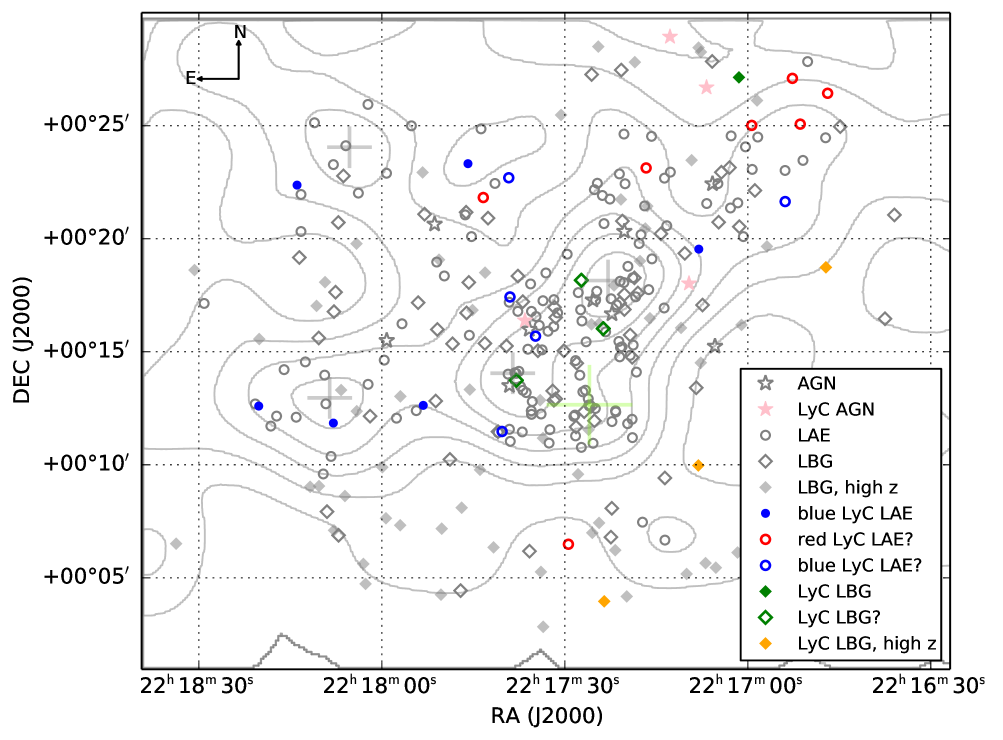
Figure 15: Spatial distribution of the samples with Yamada et al. (2012) density contours. The position of LAB01 is marked with a green cross. Also marked are the 4 highest overdensities (gray crosses). Possible LyC contaminants are shown with open markers of the corresponding shape and color.

For the IGM attenuation we use the results of the new transmission model in Inoue & Iwata (2008), but with an updated IGM absorbers’ statistics described in Inoue et al. (2014). This transmission model finds significantly smaller IGM attenuation of LyC than the Madau (1995) model. For example the cumulative probability to have an IGM attenuation of $<1$ mag in our LyC filter for galaxies at redshift $z\sim 3.1$ is $\sim 20\%$ for the Madau model but $\sim 65\%$ for the Inoue et al. (2014) model. We use the median of all sightlines, $\tau^{med}_{IGM}=0.74^{m}$, which is appropriate for general LAEs and LBGs.

Direct observation of $\left(f_{LyC}/f_{UV}\right)_{int}$ is not possible so we must obtain it from population synthesis models. For $\left(f_{LyC}/f_{UV}\right)_{obs}$ we take the values from Section 5.6, which have been statistically corrected for foreground contamination. We use a standard SB99 model with a Salpeter IMF ($\alpha=2.35$), with mass range $1$-$100$M_☉, low-metallicity ($Z=0.0004$), and $100$Myr age. The average relative escape fraction from LAEs and LBGs is shown in Table 4.

To obtain absolute $f_{esc}$, we estimate the amount of dust attenuation in the individual galaxies by comparing the average observed V$-$i^′ color of each stacking sample to dust-free model predictions. We assume the dust attenuation follows $A(1500)=10.33E(B-V)$ (Calzetti et al., 2000). With $E(B-V)=0.1$, the predicted reddening in $($V$-$i^′$)$ is then $0.199$. The average absolute $f_{esc}$ and the $A(1500)$ values are also listed in Table 4.

5.8 Spatial distribution

In Figure 15 we examine the spatial distribution of all galaxies in the sample together with the LyC candidates, superimposed on density contours from Yamada et al. (2012). There are four major overdensity peaks, with maxima $6.3,5.5,4.3,$ and $3.9$ photometric LAEs per square arcminute. All viable LyC candidates seem to occupy regions either at the edges of these concentrations or far away from any overdensity peak. This can be shown more qualitatively by looking at the distribution of minimum distances to any one of the four overdensity peaks in Figure 16. The figure shows that viable LyC candidates seem to avoid overdense regions and are instead found at distances $\gtrsim 1\arcmin\approx 450$ kpc in physical units away from any density maximum. The one LyC candidate found in the center of an overdensity peak, LBG07, is already flagged as a possible contaminant for morphological reasons in Section 3. The remaining LyC candidates are found in regions with lower spatial density compared to their parent sample. The average overdensity at the positions of the non-LyC LAEs is $\sim 3.9$, while for the LyC LAEs it is $\sim 2.7$. If we only consider viable LyC LAEs the average overdensity is $\sim 3.0$. Note that the number of LyC LBG candidates unassociated with the proto-cluster is three which is comparable to four LyC LBGs proto-cluster members if we count possible contaminants, and is three times greater if we consider only viable candidates ($3:1$). Recently, Hine et al. (2016) reported a higher merger fraction for LBGs in the SSA22 proto-cluster compared to field galaxies. A dynamical perturbation such as a merger could facilitate the building of low density tunnels and holes in the ISM which in turn possibly enables the escape of both Ly$\alpha$ and LyC. It is then noteworthy that among LBGs LyC escape remains curiously unenhanced by the dynamic high density, high merger fraction environment that comprises the SSA22 proto-cluster, and we have in fact only one viable LyC LBG candidate (LBG02) at the redshift of the proto-cluster, located very far away from any overdensity peak ($\sim 4.5$Mpc from the nearest peak). A similarly puzzling absence of LyC leaking proto-cluster LBGs can be noted in Mostardi et al. (2015), who revised their HS1549+1933 LyC detections with new multiband HST observations and found one secure LyC leaking LBG detection at a redshift of $z\sim 3.14$, clearly unassociated with the proto-cluster at $z\sim 2.85$. Higher HI column densities in the IGM of proto-clusters (Cucciati et al., 2014; Stark et al., 2015, Hayashino et al. in preparation) may be responsible for this apparent dearth of LyC LBGs in rich proto-cluster environments and could be an indication that one should instead be searching for them in the field.

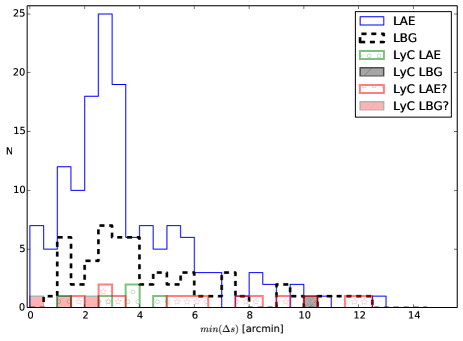
Figure 16: Distribution of minimum distances $\Delta s$, measured between a galaxy and the position of the closest overdensity peak. Only galaxies associated with the proto-cluster are included.

6 Discussion

The mechanism that allows LyC to escape could be a major merger event in which extreme dynamical disturbance of the ISM clears escape paths for the ionizing photons. Another possibility is that the star formation is instead flocculent, with high mass stars ionizing the gas and blowing holes in the ISM via strong stellar winds and/or during their supernova (SN) stage. Alternatively, the ionizing high mass stars could be formed through cold accretion of pristine gas onto the main system, with the gas compressing and forming stars before it enters the main body of the galaxy where large quantities of neutral hydrogen prevent ionizing photons from escaping. This latter scenario could account for the observed offsets between main galaxy body (in UV) and the substructures associated with the LyC leakage (Inoue et al., 2011). The LyC emission in our candidate sample comes from relatively compact clumps for both LAEs and LBGs. Spatial offsets between these clumps and the position of the galaxy in the R band are predominantly detected for LBGs (for about half of the LyC LBG sample), while few LAE show similar offsets. If not all of them are just due to the chance coincidence of foreground objects, these offset substructures could be accretion or infall of a smaller galaxy with very low metallicity, forming stars for the first time. The fact that the offset substructures are present more often for LBGs than for LAEs possibly reflects the intrinsic differences in the properties of these two types of galaxies. LBGs are generally more luminous than LAEs in rest-frame UV continuum and more massive both kinematically and in stellar populations. Additionally, the data suggest a possible correlation between LyC and Ly$\alpha$ strength. While such a correlation seemingly indicates spatial coincidence of both emissions and, consequently, no offsets, Ly$\alpha$ is a resonant line and it is possible for Ly$\alpha$ to escape the galaxy but then be scattered in the circum-galactic medium, thus showing a spatial offset from the LyC and UV emissions.

The escape fraction of LyC appears to be bimodal in nature, with some galaxies showing very large LyC emission, while others have no discernible LyC signal. The stacking analysis indicates that there is a dearth of objects with marginal LyC detections. If all galaxies leak LyC, these non-detections could be due to the viewing angle and the geometry of the distribution of the individual galaxy’s dust and gas. Alternatively, the bimodality may instead reflect an intrinsic difference in the geometry of the ISM between LyC leaking and non-LyC galaxies. The geometry may be such that it does not allow for the formation of low density tunnels. We note that if the LyC emission is extended and diffuse it would be practically invisible in our images. It is also possible that the apparent bimodality may reflect the different nature of the stellar populations. Perhaps the LyC candidates we observe are only a few special LAEs/LBGs which have exotic stellar populations whose high LyC emissivity makes them detectable in LyC.

The LBGs data indicate that the LyC candidates are dominated by a very young extremely metal-poor or Pop III stellar population. The LAE data are difficult to interpret since they are inconsistent with models which assume a standard or even a top-heavy IMF. The debate on IMF variations in the upper mass end for high-$z$ galaxies ($z\geq 3$) is ongoing in the literature (e.g., Ricotti et al., 2004; Chary, 2008; Murphy, 2011), and a top-heavy IMF at high-$z$ seems appropriate given the low metallicity environment. The situation is still unresolved, however, and constraints on the upper mass end have proven very hard to obtain. Our LyC LAEs data indicate that a dominant young and zero metallicity population seems to be a necessary feature, and further suggest that an exotic IMF comprising predominantly high-mass stars is necessary.

Our LyC LBG detection rate ($6.6\%$) is a factor of $\sim 2$ lower than that of the LyC LAEs ($13\%$), further strengthening a possible luminosity dependence for the LyC escape fraction. It may be harder for LyC to escape from LBGs, perhaps due to the lack of strong Ly$\alpha$. This is supported by the clearly lower average $EW($Ly$\alpha$$)$ for LBGs in the protocluster (Figure 10) compared to LAEs. Some of the LyC candidates show offsets between the LyC detection and the Ly$\alpha$ emission, with no discernible counterpart of Ly$\alpha$ emission at the position of the LyC detection. These could be galaxies that have recently completely exhausted their HI supply and thus are no longer making new stars. If the star formation has only recently been quenched so that massive young stars are still present and producing ionizing radiation, the galaxies would still be detectable in UV continuum observations and the lack of circum-galactic gas would facilitate the escape of LyC without an accompanying emission in Ly$\alpha$.

7 Conclusions

We present the largest to date sample of LyC candidates at any redshift with $18$ LyC LAEs and $7$ LyC LBGs from a base sample of $156$ LAEs and $134$ LBGs, with very low statistical probability that all candidates are foreground contaminated. Many LyC candidates show a spatial offset between the rest-frame UV detection and the compact LyC-emitting substructure. These vary in size (anywhere between $0$ to $\sim 1.4\arcsec$), depend on how they are measured, and could indicate infall or accretion of a smaller object, which may facilitate the escape of LyC. Although the sample number is small, especially if excluding also the possible but unconfirmed contaminants, we find evidence for a positive LyC/Ly$\alpha$ correlation, which is consistent with the idea that both types of photons benefit from the same escape route through the galaxy’s ISM.

The LyC emission seems to be bimodal - stacking non-detections reveals no significant LyC signal in either LAEs or LBGs - but are unable with the current data to decide on the nature of this seeming bimodality as it may be intrinsic or a product of the viewing angle. From stacking we obtain $3\sigma$ upper limits on the average flux density ratio, statistically corrected for foreground contamination. For LAEs we obtain $\left<f_{LyC}/f_{UV}\right><0.08$, for LBGs $\left<f_{LyC}/f_{UV}\right><0.02$. Assuming a Salpeter IMF ($\alpha=2.35$), a standard SB99 model with low metallicity $Z=0.0004$, and age $100$ Myr the $3\sigma$ upper limits on the absolute escape fractions are $f_{esc}<0.15$ and $f_{esc}<0.01$ for LAEs and LBGs, respectively.

Many of the LyC LAE candidates in our sample are very strong LyC sources, with flux density ratios $f_{LyC}/f_{UV}>1$, which are difficult to explain with standard models. They are also hard to explain as foreground contaminants, since their UV slope $\beta$ is unusually blue, $-2.7<\beta_{UV}<-3.2$.

There are indications that the dense rich environment of the proto-cluster is not hospitable to LyC LBGs, resulting in higher detection rate of viable LyC LBG candidates in the field. The spatial distribution of the LyC candidates revealed that they seemingly avoid the very dense regions around the overdensity peaks of the proto-cluster.

The possibility of foreground contamination prevents us from definitive discussion of the nature of strong LyC sources and further statistical analysis of LyC emissivity and escape fraction of star-forming galaxies at $z\gtrsim 3.1$. Sensitive spectroscopy and high spatial resolution imaging for all candidates are necessary.

Appendix A Notes on individual LyC candidates

Here we briefly summarize our analysis of the individual objects and justify the decision to treat them as viable candidates or possible contaminants. In addition, in Figure 17 we show $5\arcsec\times 5\arcsec$ cut-out images of LyC candidates with available HST ACS, WFC3/UVIS or WFC3/IR imaging. The HST data are summarized in Table 5. These data are only used for visual analysis of the visible substructure. Data from WFPC2 are too shallow to be useful. We have tried to match the coordinates of the HST image to the Subaru images with a full plate solution but in some images there seems to be a residual offset in the WCS. This is especially visible for LBG05 in the F336W image with overplotted NB359 contours. In Figure 20 we also show complementary spectra for the LyC candidates which cannot be found in the literature. Most of our sample is based on the spectroscopic sample of Steidel et al. (2003).

Table 5: Summary of the HST data^† for the LyC candidates with object ID in our catalog (ID), filter name, instrument (Inst), exposure time (Exp) in seconds, HST proposal number (P. ID), and name of principle investigator (PI). Confirmed contaminants not included.

ID	Filter	Inst	Exp	P. ID	PI
LAE08	F814W	ACS	6144	10405	S. Chapman
LAE17
LBG05
LBG06
LAE12	F160W	WFC3	2612	11735	F. Mannucci
	F625W	ACS	2208
LAE09	F814W	ACS	4670	9760	R. Abraham
LAE10			4670
LBG07			7320
LBG05	F110W	WFC3	2612	11636	B. Siana
LBG05	F160W		2612
LBG05	F336W		5300
LBG06	F336W		5300

$\dagger$ WFPC2 data not listed due to their very low exposure time.

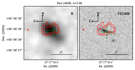
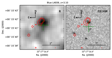
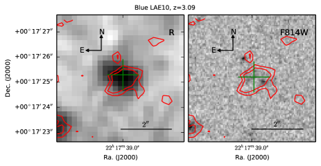
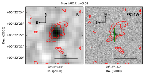
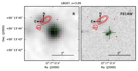
Figure 17: HST data of the LyC candidates. The intensity scales of the display are individual for each image. The green cross marks the location of the R band detection in Subaru/Suprime-Cam. The red lines are 2 and 3$\sigma$ contour levels in NB359. Passbands in HST and Subaru images are noted in the images.

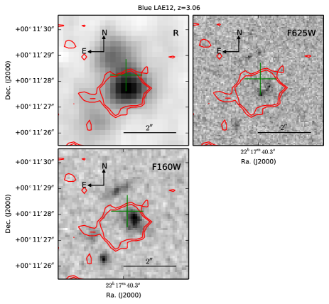
Figure 18: continued

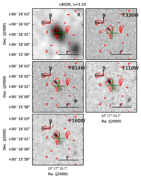
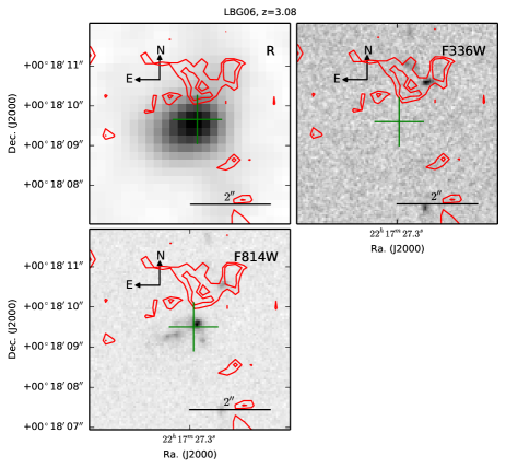
Figure 19: continued

LAE01 This object has one of the largest offsets between LyC (NB359) and Ly$\alpha$ (NB497) ($1.3$″) and we therefore flag it as a possibly but unconfirmed contaminated object.

LAE02 There are multiple components in the broadband images, but no HST data is available for higher resolution. Ly$\alpha$ (NB497) is extended in the South-East direction. In the FOCAS spectrum (Figure 20) taken at the position of LyC (NB359) emission, the strongest line is detected at $\lambda_{obs}=5021$Å. If this is Ly$\alpha$ then $z=3.123$. There is another detected line at $\lambda_{obs}=5734.8$Å, which at this redshift gives rest-frame $\lambda_{0}=1391$Å, where no major line is expected. If the strongest line is instead [OII] $\lambda_{0}=3728.3$Å then the redshift would be $z=0.347$. The second line would then be at $\lambda_{0}=4257$Å, where again, no major line is expected. Since we have an unidentified line in the spectrum we flag this object as a possibly but unconfirmed contaminated object.

LAE03 The major line in the spectrum at the LyC (NB359) emission position at $\lambda_{obs}=4969.6$Å gives $z=3.088$ if it is Ly$\alpha$ (Figure 20). There is a second line at $\lambda_{obs}=5583.9$Å, which implies $\lambda_{0}=1365.9$Å. If the strongest line is instead [OII], then $z=0.333$ and the second line would be at $\lambda_{0}=4186$Å. No major lines are expected at any of these positions. If the second line is indicating a foreground contaminant, then this object would have to be exactly aligned within the PSF with the position of the continuum in the FOCAS spectrum. Since we have an unidentified line we flag this object as a possibly but unconfirmed contaminated object.

LAE04 There is a visible counterpart in the rest-frame non-ionizing UV image (R band) to the Ly$\alpha$ emission, which is offset from the source with LyC emission by $1.3$″. Due to the large offset we flag this as a possibly but unconfirmed contaminated object.

LAE05 The primary emission line in the spectrum taken at LyC (NB359) position indicates $z=3.096$ if it is Ly$\alpha$ (Figure 20). Similarly to LAE03, there is another line at $\lambda_{obs}=7480$Å, giving $\lambda_{0}=1826$Å at this redshift. If the primary line is instead [OII], then $z=0.336$ and the secondary line is at $\lambda_{0}=5598$Å. No major lines are expected at any of these positions. The secondary line is close to a sky line and may be simply noise. Also, the contaminating object would have to be perfectly aligned with the continuum (within the PSF). This object is flagged as a possibly but unconfirmed contaminated one.

LAE06 This is object ’f’ in Inoue et al. (2011). There are no significant offsets between LyC and the reference position or the Ly$\alpha$ position, and the spectrum is clean. This is a convincing object.

LAE07 This is object ’e’ in Inoue et al. (2011). There is a large offset between broadband and Ly$\alpha$ ($0.89$″), and also between Ly$\alpha$ and LyC ($1.06$″). We flag this object as possibly contaminated by a foreground object.

LAE08 This is object ’h’ in Inoue et al. (2011). There are two distinct objects in the R image. The Ly$\alpha$ emission is associated with the object to the South-West, as seen also from the HST F814W image. The LyC (NB359) emission seems more spatially coincident with the object to the North-East. Since the Ly$\alpha$ and LyC sources are spatially different, this may be contaminated by a foreground object and we flag it as such.

LAE09 This object is a LyC candidate from Nestor et al. (2013, LAE038). We did not detect any emission in our FOCAS 2008 spectrum. The spectrum of the source spatially associated with the LyC emission has no emission line and the peak of Ly$\alpha$ emission (NB497) is offset by $0.66$″, where there is a corresponding substructure seen in the HST image (Figure 17). We therefore flag this object as a possibly but unconfirmed contaminated object.

LAE10 This is object ’b’ in Inoue et al. (2011). Ly$\alpha$ is offset and appears to be associated with a separate object seen in B and V bands, and HST F814W. We mark it as possibly contaminated.

LAE11 The UV continuum (R band) and the Ly$\alpha$ emission (NB497) are well aligned, with no offset. However, there is a large offset ($1.1$″) between Ly$\alpha$ and LyC (NB359), and consequently we flag this object as a possibly but unconfirmed contaminated object.

LAE12 The Ly$\alpha$ emission in our data is extended and appears to spatially cover both the UV and LyC positions. HST data in both F625W and F160W reveal a faint continuum “edge-on” source at the position of Ly$\alpha$ (NB497). The offset between the centroid detections of Ly$\alpha$ and LyC is large ($1.3$″) and we therefore flag this object as a possibly but unconfirmed contaminated object.

LAE13 There is a large offset between LyC and Ly$\alpha$ ($1.0$″) and also between Ly$\alpha$ and rest-frame UV ($0.85$″). We therefore flag this object as possibly contaminated by a foreground object.

LAE14 This is object ’c’ in Inoue et al. (2011). Rest-frame UV (R band) and LyC (NB359) are spatially aligned, and although there is a small ($0.8$″) offset between Ly$\alpha$ and LyC, the line is clearly visible in the spectrum, which is otherwise clean. We retain this object as a candidate due to lack of evidence to the contrary.

LAE15 This is object ’g’ in Inoue et al. (2011). The LyC detection is marginal, $3.3\sigma$ at the reference position, and $2.7\sigma$ at the position of Ly$\alpha$. There is no high resolution data for this object and we keep it as a candidate due to lack of evidence to the contrary.

LAE16 The offset between LyC and R is relatively small, $0.59$″. Ly$\alpha$ appears to be extended and there is no apparent offset from the broadband images. We keep this object as a viable candidate.

LAE17 The HST F814W image shows a counterpart to the Ly$\alpha$ emission. The offset between Ly$\alpha$ and the broadband images is, however, small. We keep this object as a viable candidate.

LAE18 UV and Ly$\alpha$ are well aligned but there is a large offset between Ly$\alpha$ and LyC ($1.2$″). We therefore flag this object as a possibly but unconfirmed contaminated one.

LBG01 We see no apparent substructure in the broadband images, but the LyC emission comes from two clumps, one with a larger offset. The spectrum is clean and this is a viable candidate.

LBG02 The LyC emission is associated with a substructure (with a $0.8$″ separation) to the North. The continuum subtracted Ly$\alpha$ is negative at the reference position but there is positive signal surrounding the position, including the location of the LyC emission. This is a viable candidate.

LBG03 The LyC emission comes from two clumps surrounding the UV continuum. The spectrum shows strong Ly$\alpha$ at $z=3.287$ and this is a viable candidate.

LBG04 The redshift for this object ($z=3.31$) was established by Steidel et al. (2003). The LyC detection is offset from the broadband by $0.8$″ and it is marginal even for measurements at the offset position ($3.1\sigma$). This object is retained as a viable candidate.

LBG05 This object is from Nestor et al. (2013), whose optical spectrum shows a Ly$\alpha$ line at $z=3.1$. They mention (but do not show) a near-IR spectrum with a possible [OIII] emission at $z=2.88$, at $0.7$″separation. This object was consequently removed from their LyC candidate list. Our FOCAS 2008 spectrum, although noisy, confirms the $z=3.102$ of the Ly$\alpha$ emission and shows no emission at Ly$\alpha$ for an assumed redshift of $z=2.88$, which is why we retain this object as a LyC candidate. The available F336W HST image shows an object well aligned with the substructure we see in our narrowband LyC image, and there is no offset between the UV peak and F336W or the narrowband LyC image. However, this object was recently flagged as a foreground contaminant by Siana et al. (2015) based on a single emission line in their near-IR spectrum of the LyC emitting substructure. We flag this object as a possibly but unconfirmed contaminated one.

LBG06 This object was treated in Nestor et al. (2013) as a confirmed LyC source, and a new investigation by Siana et al. (2015) could not definitively demonstrate contamination. However, the offset between the UV continuum and LyC emission is rather large ($1.1$″) and we flag it as a possibly but unconfirmed contaminated object.

LBG07 Our LRIS 2010 spectrum for this object is of poor quality and heavily affected by a nearby star, and no line was identified. However, this object is placed at $z=3.09$ from spectroscopy by both Steidel et al. (2003) and Nestor et al. (2013), so we consider its redshift confirmed. The HST F814W shows a diffuse counterpart to the LyC emission, however we measure a large offset ($1.3$″) between UV and LyC, and flag this object as a possibly but unconfirmed contaminated one.

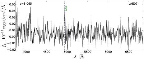
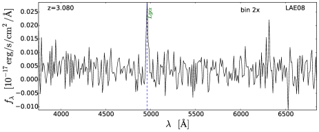
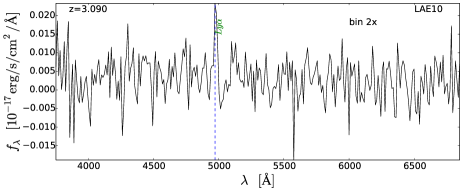
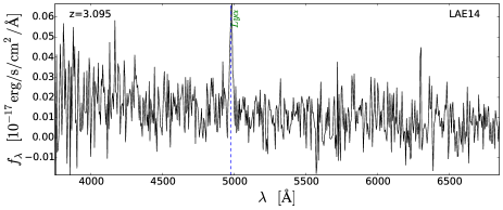
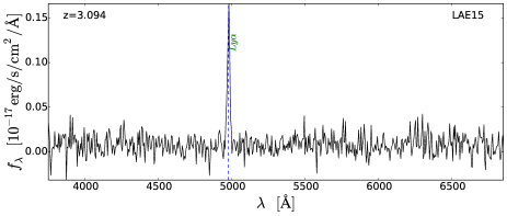
Figure 21: continued

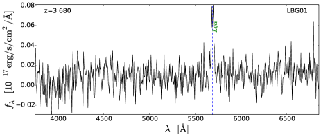
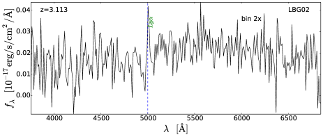
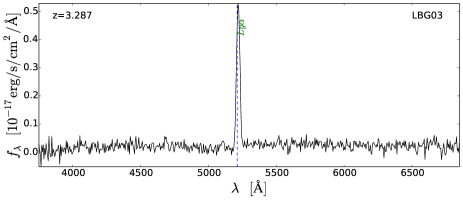
Figure 22: continued

Appendix B Brightness variability

None of the non-AGN LyC candidates show any variability in brightness over the span of 6 years. The variability test we performed involved reducing B band Suprime-Cam data of the SSA22 field taken in the years $2002$, $2003$, $2007$, $2008$. After equalizing the zeropoint between the four years we compared the resulting four magnitudes per object, which revealed no variation of LyC candidates with the exception of two LyC AGN, which show variation with high significance. From the non-LyC objects only known X-ray AGN in our sample were found to vary. More details on the variability test and its results can be found in the forthcoming paper on AGN in the SSA22 field (Micheva et al. in preparation). We show the light curves of the LAE and LBG LyC candidates in Figure 23. LAE11 is too faint in the four individual frames and is not shown. LAE18 is too faint in the frame from $2003$, and is not shown.

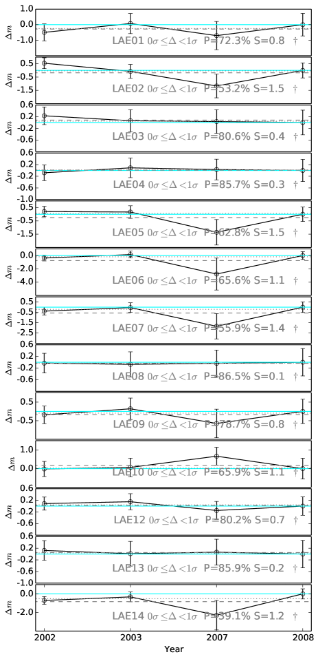
Figure 23: Light curves for all LyC candidates. The source ID is indicated for each object, as well as the variability “strength” $\Delta$ in multiples of $\sigma$, the probability of a random match to the current profile (P in percent), and the formal variability significance (S) as defined in Klesman & Sarajedini (2007). Proto-cluster association is indicated by $\dagger$. Solid cyan line is at the reference year $2008$ of $\Delta m=0$. The dotted (dashed) line is the median (average) of the 4 points. LAE11 and LAE18 are too faint in individual frames and could not be investigated.

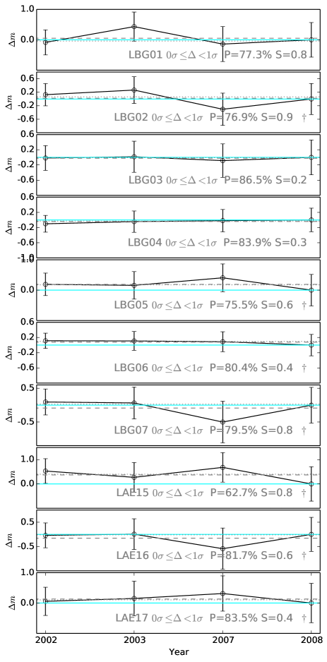
Figure 24: continued

References

- Abraham et al. (2004) Abraham R. G., Glazebrook K., McCarthy P. J., et. al. 2004, AJ, 127, 2455
- Ando et al. (2006) Ando M., Ohta K., Iwata I., et. al. 2006, ApJ, 645, L9
- Bergvall et al. (2013) Bergvall N., Leitet E., Zackrisson E., et. al. 2013, A&A, 554, A38
- Boutsia et al. (2011) Boutsia K., Grazian A., Giallongo E., et. al. 2011, ApJ, 736, 41
- Bouwens et al. (2009) Bouwens R. J., Illingworth G. D., Franx M., Chary R.-R., Meurer G. R., Conselice C. J., Ford H., Giavalisco M., van Dokkum P., 2009, ApJ, 705, 936
- Calzetti et al. (2000) Calzetti D., Armus L., Bohlin R. C., et. al. 2000, ApJ, 533, 682
- Chary (2008) Chary R.-R., 2008, ApJ, 680, 32
- Conroy & Kratter (2012) Conroy C., Kratter K. M., 2012, ApJ, 755, 123
- Cooke et al. (2014) Cooke J., Ryan-Weber E. V., Garel T., et. al. 2014, MNRAS, 441, 837
- Cowie et al. (2009) Cowie L. L., Barger A. J., Trouille L., 2009, ApJ, 692, 1476
- Cucciati et al. (2014) Cucciati O., Zamorani G., Lemaux B. C., et. al. 2014, A&A, 570, A16
- Dijkstra et al. (2014) Dijkstra M., Wyithe S., Haiman Z., et. al. 2014, MNRAS, 440, 3309
- Eldridge & Stanway (2009) Eldridge J. J., Stanway E. R., 2009, MNRAS, 400, 1019
- Forero-Romero & Dijkstra (2013) Forero-Romero J. E., Dijkstra M., 2013, MNRAS, 428, 2163
- Fumagalli et al. (2011) Fumagalli M., O’Meara J. M., Prochaska J. X., 2011, Science, 334, 1245
- Gavignaud et al. (2008) Gavignaud I., Wisotzki L., Bongiorno A., et. al. 2008, A&A, 492, 637
- Grazian et al. (2016) Grazian A., Giallongo E., Gerbasi R., et. al. 2016, A&A, 585, A48
- Gronwall et al. (2007) Gronwall C., Ciardullo R., Hickey T., et. al. 2007, ApJ, 667, 79
- Guaita et al. (2016) Guaita L., Pentericci L., Grazian A., et . al. 2016, A&A, 587, A133
- Hayashino et al. (2004) Hayashino T., Matsuda Y., Tamura H., et. al. 2004, AJ, 128, 2073
- Hine et al. (2016) Hine N. K., Geach J. E., Alexander D. M., et. al. 2016, MNRAS, 455, 2363
- Inoue (2010) Inoue A. K., 2010, MNRAS, 401, 1325
- Inoue & Iwata (2008) Inoue A. K., Iwata I., 2008, MNRAS, 387, 1681
- Inoue et al. (2006) Inoue A. K., Iwata I., Deharveng J.-M., 2006, MNRAS, 371, L1
- Inoue et al. (2011) Inoue A. K., Kousai K., Iwata I., et. al. 2011, MNRAS, 411, 2336
- Inoue et al. (2014) Inoue A. K., Shimizu I., Iwata I., et. al. 2014, MNRAS, 442, 1805
- Iwata et al. (2009) Iwata I., Inoue A. K., Matsuda Y., et. al. 2009, ApJ, 692, 1287
- Izotov et al. (2016) Izotov Y. I., Orlitová I., Schaerer D., Thuan T. X., Verhamme A., Guseva N. G., Worseck G., 2016, Natur, 529, 178
- Johnson (2010) Johnson J. L., 2010, MNRAS, 404, 1425
- Klesman & Sarajedini (2007) Klesman A., Sarajedini V., 2007, ApJ, 665, 225
- Kubo et al. (2013) Kubo M., Uchimoto Y. K., Yamada T., et. al. 2013, ApJ, 778, 170
- Kurczynski et al. (2014) Kurczynski P., Gawiser E., Rafelski M., Teplitz H. I., Acquaviva V., Brown T. M., Coe D., de Mello D. F., Finkelstein S. L., Grogin N. A., Koekemoer A. M., Lee K.-s., Scarlata C., Siana B. D., 2014, ApJ, 793, L5
- Kurucz (1993) Kurucz R. L., 1993, VizieR Online Data Catalog, 6039, 0
- Leitet et al. (2013) Leitet E., Bergvall N., Hayes M., et. al. 2013, A&A, 553, A106
- Leitet et al. (2011) Leitet E., Bergvall N., Piskunov N., et. al. 2011, A&A, 532, A107
- Leitherer et al. (1995) Leitherer C., Ferguson H. C., Heckman T. M., et. al. 1995, ApJ, 454, L19
- Leitherer et al. (2016) Leitherer C., Hernandez S., Lee J. C., Oey M. S., 2016, ArXiv e-prints
- Leitherer et al. (1999) Leitherer C., Schaerer D., Goldader J. D., et. al. 1999, ApJS, 123, 3
- Madau (1995) Madau P., 1995, ApJ, 441, 18
- Matsuda et al. (2009) Matsuda Y., Nakamura Y., Morimoto N., et. al. 2009, MNRAS, 400, L66
- Matsuda et al. (2004) Matsuda Y., Yamada T., Hayashino T., et. al. 2004, AJ, 128, 569
- Miyazaki et al. (2002) Miyazaki S., Komiyama Y., Sekiguchi M., et. al. 2002, PASJ, 54, 833
- Mostardi et al. (2013) Mostardi R. E., Shapley A. E., Nestor D. B., et. al. 2013, ApJ, 779, 65
- Mostardi et al. (2015) Mostardi R. E., Shapley A. E., Steidel C. C., et. al. 2015, ApJ, 810, 107
- Murphy (2011) Murphy E. J., 2011, in Treyer M., Wyder T., Neill J., Seibert M., Lee J., eds, UP2010: Have Observations Revealed a Variable Upper End of the Initial Mass Function? Vol. 440 of Astronomical Society of the Pacific Conference Series, Identifying Variations to the IMF at High-z Through Deep Radio Surveys. p. 361
- Nakahiro et al. (2013) Nakahiro Y., Taniguchi Y., Inoue A. K., et. al. 2013, ApJ, 766, 122
- Nakamura et al. (2011) Nakamura E., Inoue A. K., Hayashino T., et. al. 2011, MNRAS, 412, 2579
- Nestor et al. (2013) Nestor D. B., Shapley A. E., Kornei K. A., et. al. 2013, ApJ, 765, 47
- Nestor et al. (2011) Nestor D. B., Shapley A. E., Steidel C. C., et. al. 2011, ApJ, 736, 18
- Nonino et al. (2009) Nonino M., Dickinson M., Rosati P., et. al. 2009, ApJS, 183, 244
- Pickles (1998) Pickles A. J., 1998, VizieR Online Data Catalog, 611, 863
- Rauch et al. (2011) Rauch M., Becker G. D., Haehnelt M. G., et. al. 2011, MNRAS, 418, 1115
- Ricotti et al. (2004) Ricotti M., Haehnelt M. G., Pettini M., et. al. 2004, MNRAS, 352, L21
- Rovilos et al. (2009) Rovilos E., Burwitz V., Szokoly G., et. al. 2009, A&A, 507, 195
- Schaerer (2003) Schaerer D., 2003, A&A, 397, 527
- Schlafly & Finkbeiner (2011) Schlafly E. F., Finkbeiner D. P., 2011, ApJ, 737, 103
- Shapley et al. (2001) Shapley A. E., Steidel C. C., Adelberger K. L., et. al. 2001, ApJ, 562, 95
- Shapley et al. (2003) Shapley A. E., Steidel C. C., Pettini M., et. al. 2003, ApJ, 588, 65
- Shapley et al. (2006) Shapley A. E., Steidel C. C., Pettini M., et. al. 2006, ApJ, 651, 688
- Siana et al. (2015) Siana B., Shapley A. E., Kulas K. R., et. al. 2015, ApJ, 804, 17
- Siana et al. (2007) Siana B., Teplitz H. I., Colbert J., et. al. 2007, ApJ, 668, 62
- Siana et al. (2010) Siana B., Teplitz H. I., Ferguson H. C., et. al. 2010, ApJ, 723, 241
- Smith et al. (2016) Smith B. M., Windhorst R. A., Jansen R. A., et. al. 2016, ArXiv e-prints
- Stark et al. (2015) Stark C. W., White M., Lee K.-G., Hennawi J. F., 2015, MNRAS, 453, 311
- Steidel et al. (1998) Steidel C. C., Adelberger K. L., Dickinson M., et. al. 1998, ApJ, 492, 428
- Steidel et al. (2003) Steidel C. C., Adelberger K. L., Shapley A. E., et. al. 2003, ApJ, 592, 728
- Steidel et al. (2001) Steidel C. C., Pettini M., Adelberger K. L., 2001, ApJ, 546, 665
- Tornatore et al. (2007) Tornatore L., Ferrara A., Schneider R., 2007, MNRAS, 382, 945
- Uchimoto et al. (2012) Uchimoto Y. K., Yamada T., Kajisawa M., et. al. 2012, ApJ, 750, 116
- Vanzella et al. (2015) Vanzella E., de Barros S., Castellano M., et. al. 2015, A&A, 576, A116
- Vanzella et al. (2010) Vanzella E., Giavalisco M., Inoue A. K., et. al. 2010, ApJ, 725, 1011
- Vanzella et al. (2010) Vanzella E., Siana B., Cristiani S., et. al. 2010, MNRAS, 404, 1672
- Yamada et al. (2012) Yamada T., Matsuda Y., Kousai K., et. al. 2012, ApJ, 751, 29
- Yamada et al. (2012) Yamada T., Nakamura Y., Matsuda Y., et. al. 2012, AJ, 143, 79
- Zackrisson et al. (2013) Zackrisson E., Inoue A. K., Jensen H., 2013, ApJ, 777, 39