Effects of the reservoir squeezing on the precision of parameter estimation

Abstract

The effects of reservoir squeezing on the precision of parameter estimation are investigated analytically based on non-perturbation procedures. The exact analytic quantum Fisher information (QFI) is obtained. It is shown that the QFI depends on the estimated parameter and its decay could be reduced by the squeezed reservoir compared with thermal (vacuum) reservoir, in particular, if the squeezing phase matching is satisfied.

1 Introduction

The parameter estimation is one of most important ingredients in various fields of both the classical and quantum worlds [1, 2]. The task of quantum estimation is not only to determine the value of unknown parameters but also to give the precision of the value. It is a vital issue on how to improve the estimation precision which is closely related to the quantum Cramér-Rao inequality and quantum Fisher information (QFI) [3, 4, 5, 6, 7, 8, 9, 10] that determines the bound of the parameter’s sensitivity theoretically by [11, 12]

$$\delta(\phi)\geq 1/\sqrt{\nu\mathcal{F}_{\phi}},$$ (1)

where $\nu$ means the time of experiments, and

$$\mathcal{F}_{\phi}=\mathrm{Tr}(\rho_{\phi}L_{\phi}^{2})$$ (2)

is the QFI with the symmetric logarithmic derivative $L_{\phi}$ defined by $2\partial_{\phi}\rho_{\phi}=L_{\phi}\rho_{\phi}+\rho_{\phi}L_{\phi}$. Eq. (1) implies that the larger QFI means higher sensitivity of the parameter estimation.

The pioneer work on the quantum parameter estimation were proposed by Caves [13] who showed that the precision of phase estimation can beat the shot-noise limit (standard quantum limit). Later, lots of jobs with the similar aims are proposed, such as based on maximally correlated states [14], N00N states [15, 16, 17], squeezed states [18, 19], or generalized phase-matching condition [20], and so on. In practical scenarios, it is inevitable for a quantum system to interact with environments, the precision of quantum estimation will be influenced by different extents [21, 22, 23]. In recent years, enormous effects have been devoted to how to improve the precision of parameter estimation in the case of open systems. For example, the precision spectroscopy using entangled state in the presence of Markovian dephasing [24] and non-Markovian noise [25] are investigated; The QFI under decoherence channels [26] or in a quantum-critical environment [27] are analyzed; The QFI measured experimentally with photons and atoms are reported [28, 29]; It is also reported that the QFI subject to non-Markovian thermal environment [30] could show revival and retardation loss; The parameter-estimation precision in noisy systems could be enhanced by dynamical decoupling pulses [31], redesigned Ramsey-pulse sequence [32] or error correction [33] are also shown; Noisy metrology beyond the standard quantum limits is possible when the noise is concentrated along some spatial direction [34]. However, if the environment we considered is a squeezed reservoir, how the QFI is influenced by the reservoir’s parameters?

The squeezed reservoir has been widely studied in quantum information processing. For example, the squeezed light (reservoir) [35] or finite-bandwidth squeezing [36, 37] for inhibition of the atomic phase decays and its application in microscopic Fabry-Pérot cavity [38]. In addition, some other considerations of the squeezing reservoir were also discussed, such as the quantum entanglement dynamics [39], heat engine recycle [40], geometric phase observable [41], etc. The physical realization of the squeezed reservoir has also been proposed both in theory and in experiment based on various techniques such as the four-wave mixing [42], the parametric down conversion [43], the suitable feedback of the output signal corresponding to a quantum nondemolition measurement of an observable [44], control the parameter of the driven laser [45], quantum conversion of squeezed vacuum states [46] or energy-level modulation [47], the atomic systems in cavity QED [48] or dissipative optomechanics system [49] and so on. The reduction of the radiative decay of the atomic coherence in squeezed vacuum has been realized in the superconducting circuit and microwave-frequency cavity system [50].

In this paper, we will investigate the effects of reservoir squeezing on the QFI based on the non-perturbation processing [51]. We consider a phase estimation scheme which a two-level system with an imposed unknown phase interacts with a squeezed reservoir before the final optimal measurements. To find the influences induced by the reservoir, we derive the non-perturbative master equation by the path integral method [51]. In terms of the master equation, we obtain the exact analytic expression of QFI which is related to the precision of parameter estimation. It can be found that the QFI depends on the estimated parameter and the decay of QFI can be reduced by the squeezed reservoir compared with thermal (vacuum) reservoir. In particular, if the appropriate squeezing phase matching condition is satisfied, the decay of QFI can be prevented prominently by the reservoir squeezing.

This paper is organized as follows. In Sec. 2, the parameter estimation scheme is introduced and the non-perturbation master equation is obtained. In Sec. 3, the exact analytic expression of QFI for the estimated parameter is obtained and the effects of reservoir squeezing on the QFI are investigated. The conclusion are given in the end.

2 Parameter estimation scheme

2.1 The scheme

The setup of the parameter estimation is sketched in Fig. 1. The input state is a two-level superposed state $\left|\psi_{in}\right\rangle=\left(\left|e\right\rangle+\left|g\right\rangle\right)/\sqrt{2}$. After the phase gate ($U_{\phi}=\left|g\right\rangle\left\langle g\right|+e^{i\phi}\left|e\right\rangle\left\langle e\right|$) is operated on the input state $|\psi_{in}\rangle$, the output state is given by

$$\rho_{out}=U_{\phi}\left|\psi_{in}\right\rangle\left\langle\psi_{in}\right|U_{\phi}^{\dagger}.$$ (3)

Let the system ($\rho_{out}$) interacts with a squeezed reservoir, the quantum Fisher information (QFI) of the final state can be obtained via optimal measurement. The inverse of square root of the QFI is related to the precision of parameter estimation according to Eq. (1) regardless of the experiment times $\nu$.

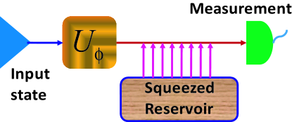
Figure 1: (Color online) The scheme of parameter estimation setup. After operated by a single qubit phase gate, the system will undergo a squeezed reservoir. The QFI can be obtained via optimal measurement.

2.2 The Hamiltonian

The initial state of the squeezed reservoir coupled to the system is given by

$$\rho_{bath} = \prod_{k}S_{k}(r,\theta)\rho_{th}S_{k}(r,\theta)^{\dagger},$$ (4)

where the squeezed operator $S_{k}(r,\theta)$ and the thermal state $\rho_{th}$ are given by

$$S_{k}(r,\theta) = \exp\left(\frac{1}{2}re^{-i\theta}b_{k}^{2}-\frac{1}{2}re^{i\theta}b_{k}^{\dagger 2}\right),$$ (5)

$$\rho_{th} = \frac{\exp(-\beta\omega_{k}b_{k}^{\dagger}b_{k})}{\mathrm{Tr}\exp(-\beta\omega_{k}b_{k}^{\dagger}b_{k})}.$$ (6)

Here $r$ is the squeezed parameter, $\theta$ is the reference phase of squeezed field and the parameter $\beta=1/(kT)$ with $k$ and $T$ denoting the Boltzsman constant and temperature, respectively. Noting that the thermal state $\rho_{th}$ will become the vacuum state $|0\rangle\langle 0|$ if the temperature $T=0$, whilst the environment will become the squeezed vacuum reservoir $\prod_{k}S_{k}(r,\theta)|0\rangle\langle 0|S_{k}(r,\theta)^{\dagger}$ [52, 53].

The total Hamiltonian of the system and reservoir reads

$$H={H_{s}}+{H_{bath}}+{H_{int}},$$ (7)

with

$${H_{s}} = {\omega_{0}}{\sigma_{z}}/2,$$ (8)

$${H_{bath}} = \sum_{k}{{\omega_{k}}b_{k}^{{\dagger}}{b_{k}}},$$ (9)

$${H_{int}} = \sum_{k}\left(g_{k}\sigma_{+}b_{k}+g_{k}^{\ast}\sigma_{-}b_{k}^{{\dagger}}\right),$$ (10)

where $\omega_{0}$ denotes the transition frequency of the two-level system, $\sigma_{\pm}$ is the raising/lowering operators of the system, $b_{k}^{\dagger}(b_{k})$ is the creation (annihilation) operators of the squeezed reservoir and $g_{k}$ is the strength of coupling between the system and environment.

2.3 The master equation of reduced density matrix

In order to get the master equation for the reduced system, we would like to employ the non-perturbative master equation which can be given, in the Schrödinger picture, by path integral method [51, 54] as

$$\frac{\partial\rho_{s}}{\partial t}=-iL_{s}\rho_{s}-\int_{0}^{t}dt^{\prime}{\left\langle{{L_{int}}{e^{i{L_{0}}({t}^{\prime}-t)}}{L_{int}}{e^{-i{L_{0}}(t^{\prime}-t)}}}\right\rangle_{bath}}{\rho_{s}},$$ (11)

where $\rho_{s}$ denotes the reduced density matrix of the system, $\left\langle\cdot\right\rangle_{bath}$ denotes the partial trace of squeezed reservoir and $L_{0}$, $L_{s}$, $L_{int}$ are the super operators defined by

$${L_{s}}\rho = [{H_{s}},\rho],$$ (12)

$${L_{0}}\rho = [{H_{s}}+{H_{bath}},\rho],$$ (13)

$${L_{int}}\rho = [{H_{int}},\rho].$$ (14)

Assuming the initial state of system plus reservoir is product state $\rho_{s}(0)\otimes\rho_{bath}$, through tedious but straightforward derivation, the non-perturbative master equation in the interaction picture can be given by

$$\frac{\partial\rho_{s}}{\partial t} = -(N+1)\alpha(t)\left(\sigma_{+}\sigma_{-}\rho_{s}-\sigma_{-}\rho_{s}\sigma_{+}\right)$$ (15)

$$-(N+1)\alpha^{\ast}(t)\left(\rho_{s}\sigma_{+}\sigma_{-}-\sigma_{-}\rho_{s}\sigma_{+}\right)$$

$$-N\alpha(t)\left(\rho_{s}\sigma_{-}\sigma_{+}-\sigma_{+}\rho_{s}\sigma_{-}\right)$$

$$-N\alpha^{\ast}(t)\left(\sigma_{-}\sigma_{+}\rho_{s}-\sigma_{+}\rho_{s}\sigma_{-}\right)$$

$$+2\left(\alpha^{\ast}(t)M\sigma_{+}\rho_{s}\sigma_{+}+\alpha(t)M^{\ast}\sigma_{-}\rho_{s}\sigma_{-}\right),$$

where the coefficients $N$ and $M$ are represented by

$$N = n\left(\cosh^{2}r+\sinh^{2}r\right)+\sinh^{2}r,$$ (16)

$$M = -\cosh r\sinh re^{i\theta}\left(2n+1\right)$$ (17)

with $n=1/(\exp(\beta\omega)-1)$ denoting average photon number.

In this paper, the structure of squeezed reservoir is supposed as the Lorentz form

$$J\left(\omega\right)=\sum_{k}\left|g_{k}\right|^{2}\delta\left(\omega_{0}-\omega_{k}\right)=\frac{\gamma}{2\pi}\frac{\lambda^{2}}{(\omega_{0}-\omega)^{2}+\lambda^{2}},$$ (18)

where $\lambda$ is the spectral width of the reservoir and connects with the reservoir correlation time as $\tau_{bath}=1/\lambda$, $\gamma$ is the decay of the system and determines the relaxation time scale as $\tau_{s}=1/\gamma$. Performing the continuum limit of the bath mode, the time correlation function can be expressed as [52]

$$\int d\omega J(\omega)e^{i(\omega_{0}-\omega)(t-t^{\prime})}=\sum_{k}\left|g_{k}\right|^{2}e^{-i\omega_{k}(t-t^{\prime})},$$ (19)

and the coefficient $\alpha(t)$ in the master equation (15) is

$$\alpha(t) = \int_{0}^{t}dt^{\prime}\int d\omega J(\omega)e^{i(\omega_{0}-\omega)(t-t^{\prime})}$$ (20)

$$= \frac{\gamma}{2}\left(1-e^{-\lambda t}\right).$$

One can prove that the non-perturbative master equation (11) coincides with the second-order time-convolutionless (TCL) master equation for the two-level system interacting with a thermal reservoir [52, 51]. Because no Markovian approximation is used, it will lead to non-Markovian dynamics for a qubits coupling to a (squeezed) thermal reservoir intuitively. However, just like the second-order TCL master equation for the two-level system interacting with vacuum reservoir, the phenomenon of temporary backflow of information [55, 56, 57, 58] cannot be revealed.

If the Markovian limit is considered, the characteristic correlation time of reservoir $\tau_{bath}$ is sufficiently shorter than the system’s $\tau_{s}$, i.e, $\tau_{bath}\ll\tau_{s}$, so the Lorentz spectrum will become a flat form, i.e., $J(\omega)=\gamma/(2\pi)$, and the coefficient $\alpha(t)=\gamma$. Thus, the widely used Markovian master equation [53, 52] can be easily obtained from the Eq. (15),

$$\frac{\partial\rho_{s}}{\partial t} = -\gamma(N+1)(\sigma_{+}\sigma_{-}\rho_{s}-2\sigma_{-}\rho_{s}\sigma_{+}+\rho_{s}\sigma_{+}\sigma_{-})$$ (21)

$$-\gamma N(\sigma_{-}\sigma_{+}\rho_{s}-2\sigma_{+}\rho_{s}\sigma_{-}+\rho_{s}\sigma_{-}\sigma_{+})$$

$$+2\gamma(M\sigma_{+}\rho_{s}\sigma_{+}+M^{\ast}\sigma_{-}\rho_{s}\sigma_{-}).$$

2.4 The solution of master equation

For the initial system state (3), the solution of the master equation given by (15) can be solved straightforward, which reads

$$\rho_{s}(t)=\left(\begin{array}[]{cc}\rho_{s}^{11}(t)&\rho_{s}^{10}(t)\\ \rho_{s}^{01}(t)&\rho_{s}^{00}(t)\end{array}\right),$$ (24)

where the elements of density matrix are

$$\rho_{s}^{11}(t) = \frac{1}{2}\left(1+A\right),$$

$$\rho_{s}^{10}(t) = \frac{1}{2}e^{\frac{i\theta}{2}}\left[\cos\left(\phi-\frac{\theta}{2}\right)B_{1}+i\sin\left(\phi-\frac{\theta}{2}\right)B_{2}\right],$$

$$\rho_{s}^{01}(t) = \rho_{s}^{10}(t)^{\ast},\rho_{s}^{00}(t)=1-\rho_{s}^{11}(t).$$ (25)

Here, the parameters $A,B_{1},B_{2}$ are given by

$$A = \frac{e^{-(1+2n)2\vartheta\cosh(2r)}-1}{(1+2n)\cosh(2r)},$$

$$B_{1} = e^{-e^{2r}(1+2n)\vartheta},$$

$$B_{2} = e^{-e^{-2r}(1+2n)\vartheta},$$

$$\vartheta = \int_{0}^{t}d\tau\alpha(\tau)=\frac{\gamma}{2}\left(t+\frac{e^{-\lambda t}-1}{\lambda}\right).$$ (26)

It is worth noting that the solution of Markovian master equation (21) can be obtained by just replacing the parameter $\vartheta$ by $\gamma t$ in Eq. (2.4).

3 Effects of reservoir squeezing on the QFI

3.1 The analytic QFI

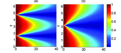
Figure 2: (Color online) The dynamics of QFI vs $\gamma t$ and $\phi$ ($\theta$). Panel (a) is under the condition $\theta=0$, and Panel (b) is under $\phi=0$. For both panels, $\lambda=0.1\gamma$, $r=1.5$ and $kT=0.5\omega$.

The explicit expression of the QFI for the estimated parameter $\phi$ is given by [6]

$$\mathcal{F}_{\phi}=\sum_{i}\frac{(\partial_{\phi}\lambda_{i})^{2}}{\lambda_{i}}+\sum_{i\neq j}\frac{2(\lambda_{i}-\lambda_{j})^{2}}{\lambda_{i}+\lambda_{j}}\left|\left\langle\varphi_{i}|\partial_{\phi}\varphi_{j}\right\rangle\right|^{2},$$ (27)

where $\lambda_{i}$ are the eigenvalues of estimated state and $\left|\varphi_{i}\right\rangle$ are the corresponding eigenvectors. For pure states, the QFI can be simplified as $\mathcal{F}_{\phi}=4\left(\left\langle\partial_{\phi}\varphi|\partial_{\phi}\varphi\right\rangle-\left|\left\langle\partial_{\phi}\varphi|\varphi\right\rangle\right|^{2}\right)$. Substituting the estimated state (24) into the formula of QFI (27), the first term of Eq. (27) is $\left(B_{1}^{2}-B_{2}^{2}\right)\sin^{2}\left(2\phi-\theta\right)/\left[m(2-m)\right]$ with $m=2\left[A^{2}+B_{1}^{2}\cos^{2}(\phi-\frac{\theta}{2})+B_{2}^{2}\sin^{2}(\phi-\frac{\theta}{2})\right]$ and the second term is $\left\{2A^{2}\left[B_{1}^{2}\sin^{2}(\phi-\frac{\theta}{2})+B_{2}^{2}\cos^{2}(\phi-\frac{\theta}{2})\right]+2B_{1}^{2}B_{2}^{2}\right\}/m$. Summing the two terms, we can obtain he analytic expression of QFI for the estimated parameter $\phi$

$$\mathcal{F}_{\phi}=\frac{B_{1}^{2}(A^{2}+B_{2}^{2}-1)-(1-A^{2})(B_{2}^{2}-B_{1}^{2})\cos^{2}(\phi-\frac{\theta}{2})}{A^{2}+B_{1}^{2}\cos^{2}(\phi-\frac{\theta}{2})+B_{2}^{2}\sin^{2}(\phi-\frac{\theta}{2})-1},$$ (28)

where the parameters $A$, $B_{1}$, $B_{2}$ are given in Eq. (2.4). From the analytic QFI (28), one can obviously find that the QFI depends on the estimated parameter $\phi$ and squeezed phasing parameter $\theta$. It varies as $\phi$ with the periodicity $\pi$, and as $\theta$ with periodicity $2\pi$ . A vivid illustrations of such relations are given by Fig. 2.

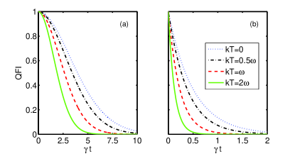
Figure 3: (Color online) QFI vs. $\gamma t$ with various temperatures without squeezing. Panel (a) is based on the master equation (15) with $\lambda=0.1\gamma$ and Panel (b) respects to the Markovian master equation (21). Here we set $kT=0$ (blue dotted line), $0.5\omega$ (black dotted-dashed line), $\omega$ (red dashed line), 2$\omega$ (green line), respectively.

3.2 The case without squeezing

In order to show the effects of the reservoir squeezing, we will first give a brief demonstration of the behavior of QFI without squeezing. That means we consider the reservoir as a standard thermal reservoir. In this case, the QFI given in Eq. (28) can be simplified as

$$\mathcal{F}_{\phi}^{th}=e^{-2(1+2n)\vartheta}.$$ (29)

The dynamics of $\mathcal{F}_{\phi}^{th}$ with different temperatures are plotted in Fig. 3 with $\lambda=0.01\gamma$ based on master equation (15) in Panel (a) and based on Markovian master equation given by Eq. (21) in Panel (b). In both conditions, one can find that the QFI with high temperature will decay more rapidly than that with low temperature. Comparing Panels (a) with (b) for the same temperature, one can also see that the QFI under Markovian limit decays faster. Consider the relation between the QFI and the precision of parameter estimation, i.e., $\delta(\phi)\geq 1/\sqrt{\nu\mathcal{F}_{\phi}}$, Fig. 3 tells that 1) the precision of parameter estimation will become lower if the reservoir gets hotter; 2) The Markovian treatment will reduce the estimation precision.

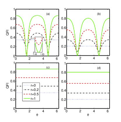
Figure 4: (Color online) QFI vs. $\phi$ at zero temperature. The QFI in Panels (a) and (c) are given under the condition $\lambda=0.1\gamma$ and $\gamma t=5$, while Panels (b) and (d) plot the QFI under the Markovian limit at $\gamma t=0.8$. The blue dotted line, black dashed-dotted line, red dashed line and green line correspond to the reservoir squeezing $r=0$, $0.2$, $0.5$, $1$, respectively. In (a) and (b), $\theta=0$, and in (c) and (d), $\phi-\frac{\theta}{2}=0.01$ is satisfied for different $\phi$ and $\theta$ all the time. The sub-Panel in (a) is the enlarged view in the vicinity of $\phi=\pi/2$.

3.3 The case with squeezing

Comparing Eqs. (28) and (29), one can find that the decay of QFI can be reduced, i.e., $\mathcal{F_{\phi}}>\mathcal{F}_{\phi}^{th}$, if the following condition for $\phi$ and $\theta$ is satisfied,

$$\cos^{2}\left(\phi-\frac{\theta}{2}\right)>\frac{(A+B_{2}^{2}-1)(B_{1}^{2}-\mathcal{F}_{\phi}^{th})}{(B_{1}^{2}-B_{2}^{2})(A_{2}^{2}+\mathcal{F}_{\phi}^{th}-1)}.$$ (30)

This implies that the decay of QFI in the squeezed reservoir can be reduced duo to the reservoir squeezing. This is obviously illustrated in Fig. 4(a) and 4(b) where the horizontal lines corresponds to the case without squeezing. It is apparent that the squeezing makes a large number of QFI surpass the horizontal lines, namely, the decay of QFI has been reduced. In particular, one can see that with the increasing of squeezing parameter $r$, the QFI is turning high and that the region below the horizontal lines is getting small. In fact, this can be easily understood in physics. In contrast to the case without squeezing, the squeezing divided the imposed phase $\phi$ into two parts respectively related to the squeezing relevant parameters $B_{1}$ and $B_{2}$ which has the opposite behaviour with $r$ (see Eq. (2.4)). When $\phi-\frac{\theta}{2}\rightarrow 0$ or $\pi$, $B_{2}$ plays the dominant role in the quantum Fisher information due to the derivative relation, which shows that the quantum Fisher information becomes large with the increasing $r$. On the contrary, $B_{1}$ will play the dominant role. This relation is obviously shown in Fig. 4 (a) and (b). That is, the competition between the $B_{1}$ and $B_{2}$ lead to the reducing or increasing the decay of the QFI under reservoir squeezing for the different regions $\phi-\frac{\theta}{2}$. From the above analysis, one can find that the squeezing phase parameter $\theta$ may play a significant role in the effects of the precision of parameter estimation. We will show it in the following.

3.4 Squeezing phase matching

From the analytic QFI of parameter $\phi$ Eq. (28), one can find that when $\phi-\frac{\theta}{2}=0$ or $\pi$, the QFI can reach the maximum with other parameters fixed. In this case, we say that $\theta$ and $\phi$ satisfy the squeezing phase matching. If the estimated phase $\phi$ happens to be in the vicinity of squeezing phase matching, i.e., $\phi-\frac{\theta}{2}\leq\delta^{\prime}$ with $\delta^{\prime}$ a small quantity, one will find that the decay of QFI will be prevented thoroughly, which can be found in Fig. 4(c) and 4(d), where we assume $\delta^{\prime}=0.01$. The most obvious role of the (approximate) squeezing phase matching in Fig. 4 is that the regions below the horizontal lines in Fig. 4(a) and Fig. 4(b) are eliminated, which is just shown in Fig. 4(c) and 4(d). In addition, one will find that in Fig. 4(c) and 4(d), the QFI with squeezing don’t depend on the estimated phase $\phi$. The reason is that we have chosen the same $\delta^{\prime}$ for all $\phi$. In fact, it is not necessary to do so. Thus we can conclude that the negative role of the reservoir squeezing could be compensated by the squeezing phase matching.

In fact, Fig. 4 illustrates the different between the cases vacuum reservoirs with and without squeezing, since we have set the temperature to be zero. In order to find out the influence of temperature accompanied by the squeezing, we plot the QFI in Fig. 5 as a function of the reservoir squeezing $r$ and the temperature $T$ at $\gamma t=10$ under condition $\lambda=0.01\gamma$ and the approximate squeezing phase matching condition $\delta^{\prime}=0.01$. It is shown that with the squeezing phase matching, the reservoir squeezing $r$ always plays the positive role in restraining the decay of QFI, but the temperature plays a negative role.

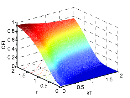
Figure 5: (Color online) QFI vs the temperature $kT$ (in the unit of $\omega$) and the squeezing parameter $r$ under condition $\lambda=0.1\gamma$ and $\gamma t=10$. Here $\phi-\frac{\theta}{2}=0.01$ is satisfied for different $\phi$ and $\theta$ all the time.

3.5 The effects of spectral property

As is mentioned previously, the master equation (15) does not reveal the phenomenon of temporary information back flow [55, 56, 57, 58]. However, it does not mean that the environment does not impact the dynamics of the QFI, which can be easily found from Eq. (27). In order to intuitively demonstrate such relations, we plot the QFI under different spectral widths $\lambda$ for $r=0.5$, $kT=0.5$ and squeezing matching condition $\phi-\frac{\theta}{2}=0.01$ in Fig. 6. One can easily find that the smaller the spectral width is, the more slowly the QFI decays.

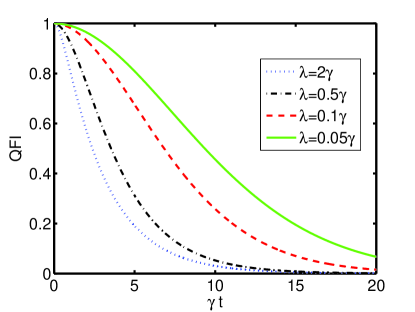
Figure 6: (Color online) QFI vs $\gamma t$ for various spectral widths. Here we set $r=0.5$, $kT=0.5$ with squeezing phase matching $\phi-\frac{\theta}{2}=0.01$ satisfied. The spectral width $\lambda$ are chosen as $\lambda=2\gamma$, $0.5\gamma$, $0.1\gamma$, $0.05\gamma$, respectively.

4 Conclusion

In summery, we have investigated the effects of reservoir squeezing on the precision of parameter estimation based on non-perturbation procedures. The exact analytic expression of the quantum Fisher information (QFI) is obtained. The QFI depends on the estimated phase $\phi$ and the reservoir squeezing parameter $r$, $\theta$. We have shown that the decay of the QFI can be reduced by the reservoir squeezing, in particular, when taking into account the squeezing phase matching.

References

- [1] V. Giovannetti, S. Lloyd, and L. Maccone, Phys. Rev. Lett. 96 (2006) 010401.
- [2] V. Giovannetti, S. Lloyd and L. Maccone, Nat. Phot. 5 (2011) 222.
- [3] H. Cramér, Mathematical Methods of Statistics (Princeton University, Princeton, NJ, 1946).
- [4] L. Pezzé and A. Smerzi, Phys. Rev. Lett. 102 (2009) 100401.
- [5] P. Hyllus, et al, Phys. Rev. A 85 (2012) 022321.
- [6] J. Ma, X, Wang, C.P. Sun, F. Nori, Phys. Rep. 509 (2011) 89.
- [7] L.J. Zhang and M. Xiao, Chin. Phys. B 22 (2013) 110310.
- [8] G.Y. Xiang and G.C Guo, Chin. Phys. B 22 (2013) 110601.
- [9] V. Giovannetti, S. Lloyd, and L. Maccone, Science 306 (2004) 1330.
- [10] K. Berrada, S.A. Khalek, and C.H. Raymond Ooi, Phys. Rev. A 86 (2012) 033823.
- [11] C.W. Helstrom, Quantum Detection and Estimation Theory (Academic Press, New York, 1976).
- [12] S.L. Braunstein and C.M. Caves, Phys. Rev. Lett. 72 (1994) 3439.
- [13] C.M. Caves, Phys. Rev. D 23 (1981) 1693.
- [14] J.J . Bollinger, W.M. Itano, D.J. Wineland and D.J. Heinzen, Phys. Rev. A 54 (1996) 4649.
- [15] K.J. Resch et al, Phys. Rev. Lett. 98 (2007) 223601.
- [16] J.A. Dunningham, K. Burnett, and S.M. Barnett, Phys. Rev. Lett. 89 (2002) 150401.
- [17] J. Joo, W.J. Munro, and T.P. Spiller, Phys. Rev. Lett. 107 (2011) 083601.
- [18] P.M. Anisimov, et al, Phys. Rev. Lett. 104 (2010) 103602.
- [19] L. Pezzé and A. Smerzi, Phys. Rev. Lett. 110 (2013) 163604.
- [20] J. Liu, X. Jing, and X. Wang, Phys. Rev. A 88 (2013) 042316.
- [21] B.M. Escher, R.L. de Matos Filho, and L. Davidovich, Nat. Phys. 7 (2011) 406.
- [22] B.M. Escher, L. Davidovich, N. Zagury, and R.L. de Matos Filho, Phys. Rev. Lett. 109 (2012) 190404.
- [23] R. Demkowicz-Dobrzański, J. Kołodyński and M. Guţă, Nature Commun. 3 (2012) 1063.
- [24] S.F. Huelga, et al, Phys. Rev. Lett. 79 (1997) 3865.
- [25] A.W. Chin, S.F. Huelga, and M.B. Plenio, Phys. Rev. Lett. 109 (2012) 233601.
- [26] J. Ma, Y.X. Huang, X. Wang, and C.P. Sun, Phys. Rev. A 84 (2011) 022302.
- [27] Z. Sun, J. Ma, X.M. Lu,and X. Wang, Phys. Rev. A 82 (2010) 022306.
- [28] R. Krischek, et al, Phys. Rev. Lett. 107 (2011) 080504.
- [29] H. Strobel, et al, Science 345 (2014) 424.
- [30] K. Berrada, Phys. Rev. A 88 (2013) 035806.
- [31] Q.S. Tan, Y. Huang, X. Yin, L.M. Kuang, and X. Wang, Phys. Rev. A 87 (2013) 032102.
- [32] L. Ostermann, H. Ritsch, and C. Genes, Phys. Rev. Lett. 111 (2013) 123601.
- [33] W. Dür, M. Skotiniotis, F. Fröwis, and B. Kraus, Phys. Rev. Lett. 112 (2014) 080801.
- [34] R. Chaves, J.B. Brask, M. Markiewicz, J. Kołodyński, and A. Acín, Phys. Rev. Lett. 111 (2013) 120401.
- [35] C.W. Gardiner, Phys. Rev. Lett. 56 (1986) 1917.
- [36] A.S. Parkins and C.W. Gardiner, Phys. Rev. A 37 (1988) 3867.
- [37] A.S. Parkins, P. Zoller and H.J. Carmichael, Phys. Rev. A 48 (1993) 758.
- [38] A.S. Parkins and C.W. Gardiner, Phys. Rev. A 40 (1989) 3796.
- [39] M.M. Ali, P.W. Chen, and H.S. Goan, Phys. Rev. A 82 (2010) 022103.
- [40] X.L. Huang, T. Wang, and X.X. Yi, Phys. Rev. E 86 (2012) 051105.
- [41] A. Carollo, et al, Phys. Rev. Lett. 96 (2006) 150403.
- [42] R.E. Slusher, L.W. Hollberg, B. Yurke, J.C. Mertz, and J.F. Valley, Phys. Rev. Lett. 55 (1985) 2409.
- [43] L.A. Wu, H.J. Kimble, J.L. Hall, and H. Wu, Phys. Rev. Lett. 57 (1986) 2520.
- [44] P. Tombesi and D. Vitali, Phys. Rev. A 50 (1994) 4253.
- [45] N. Lütkenhaus, J.I. Cirac, and P. Zoller, Phys. Rev. A 57 (1998) 548.
- [46] C. Vollmer, et al, Phys. Rev. Lett. 112 (2014) 073602.
- [47] E. Shahmoon and G. Kurizki, Phys. Rev. A 87 (2013) 013841.
- [48] T. Werlang, R. Guzmán, F.O. Prado, and C.J. Villas-Bôas, Phys. Rev. A 78 (2008) 033820.
- [49] W.J. Gu, G.X. Li and Y.P. Yang, Phys. Rev. A 88 (2013) 013835.
- [50] K.W. Murch, et al, Nature 499 (2013) 62.
- [51] A. Ishizaki, Y. Tanimura, Chem. Phys. 347 (2008) 185.
- [52] H.P. Breuer and F. Petruccione, The Theory of Open Quantum Systems (Oxford University Press, New York, 2002).
- [53] M. O. Scully and M. S. Zubairy, Quantum Optics (Cambridge University Press, Cambridge, 1997)
- [54] F.Q. Wang, Z.M. Zhang, and R.S. Liang, Chinese Phys. B 18 (2009) 0597.
- [55] H.P. Breuer, Phys. Rev. A 70 (2004) 012106.
- [56] H.P. Breuer, E.M. Laine,and J. Piilo, Phys.Rev.Lett. 103 (2009) 210401.
- [57] E.M. Laine, J. Piilo,and H.P. Breuer, Phys. Rev. A 81 (2010) 062115.
- [58] X.M Lu, X. Wang, and C.P. Sun, Phys. Rev. A 82 (2010) 042103.