Quantum criticality of bosonic systems with the Lifshitz dispersion

Abstract

We study the quantum criticality of the Lifshitz $\varphi^{4}$-theory below the upper critical dimension. Two fixed points, one Gaussian and the other non-Gaussian, are identified with zero and finite interaction strengths, respectively. At zero temperature the particle density exhibits different power-law dependences on the chemical potential in the weak and strong interaction regions. At finite temperatures, critical behaviors in the quantum disordered region are mainly controlled by the chemical potential. In contrast, in the quantum critical region critical scalings are determined by temperature. The scaling ansatz remains valid in the strong interaction limit for the chemical potential, correlation length, and particle density, while it breaks down in the weak interaction one. As approaching the upper critical dimension, physical quantities develop logarithmic dependence on dimensionality in the strong interaction region. These results are applied to spin-orbit coupled bosonic systems, leading to predictions testable by future experiments.

Introduction.—

Quantum phase transitions, uniquely driven by quantum fluctuations, appear when the ground state energy encounters non-analyticity via tuning a non-thermal parameter. Physical properties around quantum critical points (QCPs) are of extensive interests because the interplay between quantum and thermal critical fluctuations strongly influence the dynamical and thermodynamic quantities, giving rise to rich quantum critical properties beyond the classical picture Spe (2010); Sachdev (2011). Quantum critical fluctuations are believed to be responsible for various emergent phenomena, including the non-Fermi liquid behaviors in heavy fermion systems, unconventional superconductivity, and novel spin dynamics in one-dimensional quantum magnets Sachdev and Keimer (2011); Gegenwart et al. (2008); Kinross et al. (2014); Wu et al. (2014).

The progress of ultra-cold atom physics with the synthetic spin-orbit (SO) coupling has attracted a great deal of interests Zhou et al. (2013); Goldman et al. (2014); Wu et al. (2011a); Stanescu et al. (2008); Gopalakrishnan et al. (2011); Ho and Zhang (2011); Yip (2011); Li et al. (2015); Lin et al. (2009a, b); Radić et al. (2015); Huang et al. (2016). In solid state systems, the SO coupled exciton condensations have also been investigated in semiconductor quantum wells Wu et al. (2011a); Yao and Niu (2008); High et al. (2013, 2012). For bosons under the isotropic Rashba SO coupling, the single-particle dispersion displays a ring minima in momentum space. Depending on interaction symmetries, either a striped Bose-Einstein condensation (BEC), or, a ferromagnetic condensate with a single plane-wave, develops Wu et al. (2011a); Wang et al. (2010); Gopalakrishnan et al. (2011); Ho and Zhang (2011); Yip (2011); Hu et al. (2012). The case of the spin-independent interaction is particularly challenging: The striped states are selected through the “order-from-disorder” mechanism from the zero-point energy beyond the Gross-Pitaevskii framework Wu et al. (2011a). Inside harmonic traps, the skyrmion-type spin textures appear accompanied by half-quantum vortices Wu et al. (2011a); Hu et al. (2012), and the experimental signatures of spin textures have already been observed High et al. (2013, 2012).

Compared to the conventional superfluid BEC phases Weichman et al. (1986); Weichman (1988); Fisher and Hohenberg (1988); Fisher et al. (1989); Kolomeisky and Straley (1992); Sachdev et al. (1994), the progress of SO coupled bosons paves down a way to study novel quantum criticality. Consider an interacting Bose gas under the Rashba SO and Zeeman couplings: When the Zeeman field is tuned to a “critical” value, the dispersion minimum comes back to the origin exhibiting a novel $q^{4}$-dispersion Po and Zhou (2015), which is referred as the Lifshitz-point in literature Ardonne et al. (2004). Quantum wavefunctions at the Lifshitz-point exhibit conformal invariance Ardonne et al. (2004); Hsu and Fradkin (2013); Henley (1997), which have been applied to describe the Rokhsar-Kivelson point Rokhsar and Kivelson (1988) of the quantum dimer model and quantum 8-vertex model. For the SO coupled bosons, by employing an effective non-linear $\sigma$-model method, it is argued that at the Lifshitz point, a quasi-long-range ordered ground state instead of a true BEC develops due to the divergent phase fluctuations. Po and Zhou (2015).

The SO coupled bosons are not the only system to realize the Lifshitz dispersion. It has an intrinsic connection to a seemingly unrelated field of quantum frustrated magnets. Suppose a spin-$\frac{1}{2}$ antiferromagnetic Heisenberg model defined in the square lattice with the nearest-neighbor coupling $J_{1}$ and the next-nearest-neighbor coupling $J_{2}$. It can be mapped to a hard-core boson model, and the Lifshitz dispersion appears at $J_{2}=J_{1}/2$. These bosonic systems are fundamentally different from the regular ones with the quadratic dispersion: They are beyond the paradigm of the “no-node” theorem, or, Perron-Frobenius theorem Feynman (1972); Wu (2009), or, the Marshall-sign rule in the context of quantum antiferromagnetism Marshall (1955).

In this article, we investigate the quantum complex $\varphi^{4}$-theory with the Lifshitz dispersion below the upper critical dimension. There exist two fixed points (FPs) – an unstable Gaussian FP and a non-Gaussian one with a finite interaction strength. Quantum critical behaviors at both zero and finite temperatures around these two FPs are investigated. At zero temperature the particle density shows power-law dependence on the chemical potential with different exponents in the weak and strong interaction regions. At finite temperatures, according to whether the chemical potential or temperature controls the critical scalings, the disordered phase falls into the quantum disordered or quantum critical regions, respectively. In the quantum disordered region the power-law dependence of the chemical potential dominates the critical behaviors, and thermal fluctuations generate exponentially small corrections. While in the quantum critical region, physical quantities, including the chemical potential, correlation length, and particle density, exhibit power-law dependence on temperature. The scaling ansatz Sachdev (2011) breaks down in the weak interaction limit but is sustained in the strong interaction one. Logarithmic critical behaviors appear in both regions when the system is near the upper critical dimension. The connection of these results to the two-dimensional (2D) SO coupled bosonic systems is discussed.

Quantum Lifshitz $\varphi^{4}$-model.—

We construct the $d$-dimensional Euclidean quantum Lifshitz $\varphi^{4}$-action as

$$S_{0} = T\sum\limits_{\omega_{n}}{\int_{0}^{\Lambda}{d^{d}q\varphi^{*}(-i\omega_{n}-\mu+q^{4})\varphi}},$$

$$S_{I} = \frac{u}{2}\int_{0}^{\beta}{d\tau\int_{1/\Lambda}^{\infty}{d^{d}x\left|{\varphi(x,\tau)}\right|^{4}}},$$ (1)

where $d$ is the spatial dimension; $\Lambda$ is the ultra-violet (UV) momentum cut off; $\mu$ and $u$ denote the chemical potential and interaction strength, respectively; $\tau$ is the imaginary time and $\beta=1/T$; $\omega_{n}=2n\pi T$ is the Matsubara frequency; ${\varphi(x,\tau)}$ is a complex bosonic field. Due to the $q^{4}$-dispersion, the classical dimensions of $T$ and $\mu$ are $\Lambda^{4}$, and that of $u$ is $\Lambda^{\varepsilon}$ where $\varepsilon=4-d$, and thus the upper critical (spatial) dimension $d_{c}=4$. In the following, we rescale $T,\mu$ and $u$ by their classical dimensions to be dimensionless. For quantities of the correlation length, particles density, ground state energy that will be studied below, they are also rescaled by $\Lambda^{-1}$, $\Lambda^{d}$, and $\Lambda^{4}$ to be dimensionless, respectively.

The zero temperature renormalization group (RG) equations are derived following the momentum-shell Wilsonian method as presented in the Supplemental Material (SM) Sup , Sec. A. Two fixed points (FPs) are identified as a Gaussian FP $(\mu^{*}_{1},u^{*}_{1})=(0,0)$ and a non-Gaussian one $(\mu^{*}_{2},u^{*}_{2})=(0,2\varepsilon/K_{d})$ appearing at $d<d_{c}$. The RG equations are integrated as,

$$\mu_{l} = e^{4l}\mu,\ \ \ u_{l}=e^{\varepsilon l}u/C_{d}(\mu,u,l),$$ (2)

with $l$ being the RG scale parameter. $\mu_{l=0}=\mu$, $u_{l=0}=u$, and $C_{d}(\mu,u,l)=1-\frac{u}{8}K_{d}[\Phi(\mu,1,\varepsilon/4)-e^{\varepsilon l}\Phi(\mu_{l},1,\varepsilon/4)]$ where $K_{d}=2^{-d+1}\pi^{-d/2}/\Gamma(\frac{d}{2})$ with $\Gamma(z)$ being the Gamma function, and $\Phi(\mu,s,\frac{\varepsilon}{4})\equiv\sum\limits_{k=0}^{\infty}{\mu^{k}(k+\frac{\varepsilon}{4})^{-s}}$ the Hurwitz Lerch transcendent. $\Phi(\mu,s,\frac{\varepsilon}{4})$ has a branch cut running from $(+1,+\infty)$ in the complex $\mu$-plane. Since $|\mu_{l}|<1$ is maintained throughout the RG process, $u_{l}$ remains analytic as a function of $\mu$ . Furthermore, in the complex $\varepsilon$-plane, $\Phi$ has a branch cut from $(-\infty,0)$, therefore, $\varepsilon$ can be analytically extended to a finite positive value.

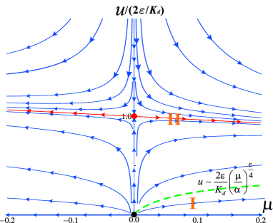
Figure 1: Diagram of the zero temperature RG flows. The red and black dots mark the two FPs. Quantum phase transitions occur when $\mu$ changes sign: The disordered and ordered phases lie at $\mu<0$ and $\mu>0$, respectively. For $\mu>0$, symbols I and II denote the weak and strong interaction regions, respectively. The dashed line at $\mu>0$ marks the crossover between these two regions.

The Gaussian FP is unstable at $\varepsilon>0$. Close to this FP, the correlation length diverges as $\xi(T=0,\mu)\approx|\mu|^{-\nu}$ with the critical exponent $\nu=1/4$ rather than $1/2$ as a consequence of the Lifshitz dispersion. At the non-Gaussian FP, $\nu=1/4$ remains at the one-loop level since the interaction does not renormalize the chemical potential at zero temperature, which is different from the Wilson-Fisher FP of the classic phase transition.

	$u$	$u_{l_{0}^{*}}$	$n$	$e_{g}$
I	$\leavevmode\nobreak\ \leavevmode\nobreak\ u\ll\frac{{2\varepsilon}}{{K_{d}}}{\left(\frac{\mu}{\alpha}\right)^{\varepsilon/4}}\leavevmode\nobreak\ \leavevmode\nobreak\$	$\leavevmode\nobreak\ \leavevmode\nobreak\ {{u}}{\left(\frac{\alpha}{\mu}\right)^{\varepsilon/4}}\leavevmode\nobreak\ \leavevmode\nobreak\$	$\leavevmode\nobreak\ \leavevmode\nobreak\ \mu/u\leavevmode\nobreak\ \leavevmode\nobreak\$	$\leavevmode\nobreak\ \leavevmode\nobreak\ \mu/2\leavevmode\nobreak\ \leavevmode\nobreak\$
II	$u\gg\frac{{2\varepsilon}}{{K_{d}}}{\left(\frac{\mu}{\alpha}\right)^{\varepsilon/4}}$	$2\varepsilon/K_{d}$	$\frac{K_{d}\alpha^{\varepsilon/4}}{2\varepsilon}\mu^{d/4}$	$\frac{\mu d}{4+d}$

Table 1: Critical properties in the weak and strong interaction regions. $\mu$ is close to the phase boundary marked by $\mu=0$. $e_{g}=\frac{1}{n}\int{\mu dn}$ gives the ground state energy density.

We consider the critical behaviors at zero temperature. The RG flows based on Eq. (2) are presented in Fig. 1. The run-away flows indicate two stable phases: one disordered at $\mu<0$ and the other ordered at $\mu>0$. The disordered phase shows vanishing particle density at the one-loop level, nevertheless, small but finite particle density could develop beyond one-loop at $u>0$. The two FPs obtained above lie on the phase boundary of $\mu=0$. To study the critical physics at $\mu>0$, a stop scale $l_{0}^{*}$ is introduced at which $\mu_{l_{0}^{*}}=\alpha\ll 1$. $\alpha$ is a non-universal parameter to control the RG flow remaining in the crossover from the critical to non-critical regions Sachdev et al. (1994). According to different behaviors of the interaction strength $u_{l_{0}^{*}}$, we define the weak and strong interaction regions via $u_{l_{0}^{*}}\approx u(\frac{\alpha}{\mu})^{\frac{\varepsilon}{4}}$, or, $u_{2}^{*}$, respectively. Correspondingly, the crossover between these two regions is approximately marked by the line of $u\approx\frac{2\varepsilon}{K_{d}}(\frac{\mu}{\alpha})^{\frac{\varepsilon}{4}}$. The critical behaviors of the particle density $n$ and the ground state energy density $e_{g}$ as well as $u_{l_{0}^{*}}$ in these two regions are summarized in Table 1 [SM Sec. A].

The finite-temperature RG equations are presented in SM Sec. B. We focus on two parts of the disordered region close to the QCPs: The quantum disordered region with negative and large chemical potential, i.e., $\mu<0$ and $|\mu|\gg T$, and the quantum critical region with small chemical potential $|\mu|\ll T$. Since the RG process ceases to work at $\mu_{l^{*}}=-1$, a stop scale $l^{*}$ is accordingly defined at which the coarse-graining length scale reaches the correlation length $\xi(T,\mu)$.

In the quantum disordered region, the running temperature remains low at the stop scale $l^{*}$, i.e., $T_{l^{*}}\ll 1$. Similar to the zero temperature case, two different limits of the running interaction strength are introduced, corresponding to the weak and strong interaction regions set by $u_{l^{*}}\approx u\mu^{-\frac{\varepsilon}{4}}$ and $u_{2}^{*}$, respectively. As shown in SM Sec. C, the correlation length is calculated as $\xi(T,\mu)\approx|\mu|^{-1/4}\left[1-c(T,u)\frac{T}{|\mu|}e^{-2\frac{|\mu|}{T}}\right]$, where $c(T,u)=\frac{1}{8}uK_{d}T^{-\frac{\varepsilon}{4}}$ and $\epsilon/4$ for the weak and strong interaction regions, respectively. The finite temperature corrections are exponentially small.

Next consider the quantum critical region (QCR) where $T\gg|\mu|$. Then at the stop scale $l^{*}$ with $\mu_{l^{*}}=-1$, $T_{l^{*}}\gg 1$, indicating that the system flows into the high-temperature region. For simplicity, we set $\mu=0$ (QCP) since in this region the correction to thermodynamic quantities from a finite $\mu$ is sub-leading. The correlation length, and particle density are denoted as $\xi_{T}$ and $n_{T}$, respectively. Similarly, based on the interaction strength $u_{l^{*}}$ the critical behaviors at finite temperatures also fall into weak and strong interaction regions characterized by $u_{l^{*}}\approx u\left[{\varepsilon}/{(2K_{d}uT)}\right]^{\frac{\varepsilon/4}{1+\varepsilon/4}}$ and $u_{2}^{*}$, respectively. The crossover line qualitatively follows $u\sim\varepsilon T^{\varepsilon/4}$.

Weak interaction region in the QCR.—

In this region, under the condition $\ln[1/(uT)]\gtrsim 1/\varepsilon$, $\xi_{T}$ and $n_{T}$ are derived in SM Secs. (D,E) as

$$\xi_{T}\approx\left[\frac{\varepsilon}{2K_{d}uT}\right]^{\frac{1}{4+\varepsilon}},n_{T}\approx a_{d}\left[\frac{\varepsilon}{2K_{d}u}\right]^{\frac{\varepsilon/4}{{1+\varepsilon/4}}}\leavevmode\nobreak\ T^{\frac{1}{{1+\varepsilon/4}}},\ \ \,$$ (3)

where $a_{d}=\frac{1}{8}K_{d}[\psi((4+d)/8)-\psi(d/8)]$ with $\psi(z)=d\ln\Gamma(z)/dz$ being the digamma function. In this case, even though the interaction is relevant, $u_{l^{*}}$ remains small, leaving a weak interaction window to justify the RG calculation. The weak interaction results in Eq. (3) can also be obtained following the one-loop self-consistent method, whose details are presented in SM Sec. D.

The scaling ansatz is believed to be valid for the system below the upper critical dimension Sachdev (2011). In our case, it dictates that the critical behavior of the correlation length in the QCR can be cast into the form, $\xi_{T}\propto T^{-1/4}g({|\mu|}/{T})$, where $g(x)$ is a universal scaling function Sachdev et al. (1994); Sachdev (2011). Then in the QCR, by setting $\mu=0$, the scaling ansatz predicts $\xi_{T}\sim T^{-1/4}$. Nevertheless, Eq. (3) yields a novel thermal exponent for the temperature dependence of $\xi_{T}$ as $\nu_{T}=1/(4+\varepsilon)$ beyond the scaling ansatz. In contrast, typically scaling-ansatz-breakdown behaviors are observed in systems equal to or above the upper critical dimension Wu et al. (2011b, 2016).

When approaching the upper critical dimension $d_{c}$, such that $\frac{{\Gamma(d/4,1)}}{{T^{\varepsilon/4}}}\ll\ln\left({\frac{2}{{K_{d}uT}}}\right)\ll\frac{4}{\varepsilon}$, the critical scalings are obtained in SM. Sec. D as

$$\xi_{T} \approx \left(\frac{K_{d}uT}{2}\ln\frac{2}{K_{d}uT}\right)^{-\frac{1}{4}},$$ (4)

$$n_{T} \approx a_{d}T\left(\frac{K_{d}uT}{2}\ln\frac{2}{K_{d}uT}\right)^{-\frac{\varepsilon}{4}},$$ (5)

which exhibit the expected non-universal logarithmic behaviors.

Based on Eqs. (3,4,5), the limits of $u\to 0$ and $\varepsilon\to 0$ of $\xi_{T}$ and $n_{T}$ do not commute, reflecting the singular nature of the QCP. At finite temperatures $\xi_{T}$ and $n_{T}$ diverge as $u\to 0$ at $\mu=0$ (QCP), which signals the strong instability around the unstable Gaussian FP. Thermal fluctuations are enhanced by the Lifshitz dispersion near the QCP due to the divergence of single-particle density of states. Both divergences are cut off when the system has a finite $\mu$ and/or a finite interaction strength.

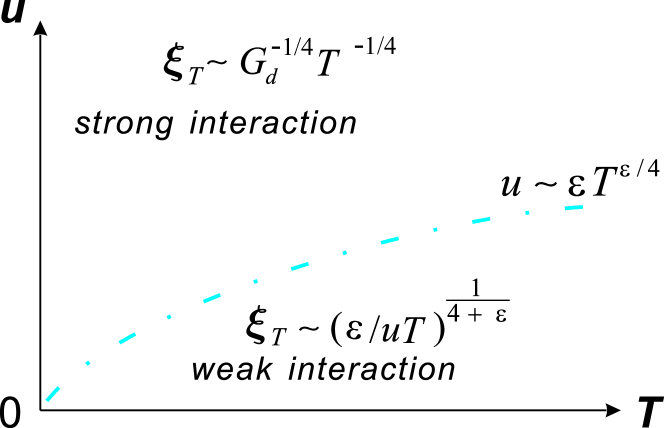
Figure 2: A sketchy illustration for the quantum critical behaviors in the QCR at $\mu=0$ with a finite $\varepsilon$. The blue dot-dashed line shows the crossover between the weak and strong interaction regions.

Strong interaction limit in the QCR.—

In this limit, $u\gg 2\varepsilon/K_{d}$, $\xi_{T}$ and $n_{T}$ exhibit power-law scalings as [SM Sec. E],

$$\xi_{T}\approx G_{d}^{-1/4}T^{-1/4},\;\ \ \,n_{T}\approx a_{d}G_{d}^{-1}T^{d/4},$$ (6)

where $G_{d}=\varepsilon\{A+\ln[(1+A\varepsilon)/(A\varepsilon)]\}$ and $A\approx 0.46$. It indicates universal scaling behaviors near the non-Gaussian FP, obeying the scaling ansatz Sachdev (2011). Interestingly, at $\varepsilon\ll 1$, Eq. (6) shows a non-analytic logarithmic dependence on $\varepsilon$ as

$$\xi_{T}\approx T^{-\frac{1}{4}}[\varepsilon\ln(1/\varepsilon)]^{-\frac{1}{4}},\ \ \,n_{T}\approx a_{d}T^{\frac{d}{4}}[\varepsilon\ln(1/\varepsilon)]^{-\frac{\varepsilon}{4}}.$$ (7)

The above discussion for finite $\varepsilon$ in the QCR is summarized in Fig. 2. The effective interaction strength is actually temperature-dependent. Increasing temperature enhances thermal fluctuations, which subdues quantum fluctuations generated from the interaction. In contrast, when decreasing temperatures, the system gradually enters a strong interaction region as long as $u>0$.

Lifshitz Bose gas from SO coupling.—

We apply the above general analysis to the 2D boson system with the Lifshitz dispersion – the SO coupled bosons under the Zeeman field. As shown in SM Sec. F, tuning the Zeeman field and SO coupling strength $\lambda$ can convert the single-particle dispersion into the form, $\varepsilon_{q}=-\mu+\frac{{q^{4}}}{{4\lambda^{2}}}$. $\lambda$ can be used to re-scale all quantities in the system by $\varphi(\omega_{n},\vec{q})/(4\lambda^{2})\to\varphi(\omega_{n},\vec{q}),\;4\lambda^{2}\mu\to\mu,\;4\lambda^{2}T\to T,\;4\lambda^{2}u\to u,\;\vec{q}\to\vec{q}$. Accordingly the low-energy physics is effectively described by the quantum Lifshitz action Eq. (1) at $d=2$.

	$u$	$u_{l^{*}}$	$n$	$e_{g}$
I	$\leavevmode\nobreak\ \leavevmode\nobreak\ u\ll 8\pi\sqrt{\frac{\mu}{\alpha}}\leavevmode\nobreak\ \leavevmode\nobreak\$	$\leavevmode\nobreak\ \leavevmode\nobreak\ u\sqrt{\frac{\alpha}{\mu}}\leavevmode\nobreak\ \leavevmode\nobreak\$	$\mu/u$	$\mu/2$
II	$u\gg 8\pi\sqrt{\frac{\mu}{\alpha}}$	$\leavevmode\nobreak\ \leavevmode\nobreak\ 8\pi\leavevmode\nobreak\ \leavevmode\nobreak\$	$\leavevmode\nobreak\ \leavevmode\nobreak\ \frac{1}{8\pi}\sqrt{\alpha\mu}\leavevmode\nobreak\ \leavevmode\nobreak\$	$\leavevmode\nobreak\ \leavevmode\nobreak\ \mu/3\leavevmode\nobreak\ \leavevmode\nobreak\$

Table 2: The zero temperature critical properties of the 2D SO coupled bosons with the Lifshitz dispersion. $\mu$ is close to the phase boundary.

At zero temperature, we focus on the region at $\mu>0$. According to the previous analysis, when $\mu$ is close to the phase boundary, the crossover between the weak and strong interaction regions is characterized by $u\approx 8\pi\left(\frac{\mu}{\alpha}\right)^{1/2}$. The critical behaviors are summarized in Table. 2. In the weak interaction region, $\mu=un$ following the mean-field result, and in the strong interaction regime, $n\propto\sqrt{\mu}$. In comparison, for the 2D bosons with the $q^{2}$-dispersion Sachdev et al. (1994), $n\approx\frac{\mu}{8\pi}\ln\frac{\alpha}{\mu}$ at $\mu\ll\Lambda^{2}$. The relation of $n\propto\sqrt{\mu}$ is similar to that of 1D bosons with the $q^{2}$-dispersion in the low density regime Affleck (1990); Sørensen and Affleck (1993); Sachdev et al. (1994). Such systems are well-known to be renormalized into the strong interaction region, nearly fermionized. This relation is also similar to a free 2D Fermi gas with the same $q^{4}$-dispersion, whose single-particle density of states also exhibits the 1D-like feature as $\rho(\varepsilon)\propto\varepsilon^{-\frac{1}{2}}$. Thus the dominant critical physics carries certain features of fermions. Similar fermionization behaviors in the strongly interacting boson systems have also been studied in the SO coupled BEC systems whose energy minima lies in a ring in momentum space Sedrakyan et al. (2012), and also in the region of resonance scattering Zhou and Mashayekhi (2013); Jiang et al. (2014).

Similar analysis can also be applied to the ground state energy density $e_{g}$. When $u$ is sufficiently small, $e_{g}\approx\mu/2\approx nu/2$ coincides with the leading order result of the usual weak-interacting dilute Bose gas with the $q^{2}$-dispersion Kolomeisky and Straley (1992). However, in the strong interaction region, $e_{g}\approx\mu/3\approx(8\pi n)^{2}/(3\alpha)$, which is very different from $4\pi n/[\ln{1/(4\pi n)}]$ for the case of the $q^{2}$-dispersion.

At finite temperatures, we focus on $\mu=0$ in the QCR of the 2D boson system. The crossover between the weak and strong interaction regions now becomes $u\approx 2T^{1/2}$. In the weak interaction region,

$$\xi_{T}\sim(uT)^{-\frac{1}{6}},\ \ \,n_{T}\sim u^{-\frac{1}{3}}T^{\frac{2}{3}},$$ (8)

showing the divergences of $\xi_{T}$ and $n_{T}$ as $u\to 0$. In cold atom experiments, interactions are typically weak in the absence of Feshbach resonances, therefore, the thermal exponent $\nu_{T}=1/6$ could be measurable. Furthermore, these scaling relations deviate from the double logarithmic behaviors of 2D boson gases with the $q^{2}$-dispersion Sachdev et al. (1994). In contrast, in the strong interaction region,

$$\xi_{T}\sim T^{-\frac{1}{4}},\ \ \ n_{T}\sim T^{\frac{1}{2}}.$$ (9)

$\xi_{T}$ is nearly determined by thermal fluctuations independent on the interaction strength. It can be understood as a decoherent effect from the strong inter-particle scattering.

Discussion and Conclusions.—

We have studied the quantum critical properties of a complex $\varphi^{4}$-model with the Lifshitz dispersion. At zero temperature, the particle density depends on the chemical potential as $n\propto\mu$ and $\mu^{\frac{d}{4}}$ in the weak and strong interaction regions controlled by the Gaussian and non-Gaussian FPs, respectively. At finite temperatures, the correlation length in the quantum disordered region scales as $|\mu|^{-\frac{1}{4}}$ in both weak and strong interaction limits, while the finite temperature corrections are exponentially small. In the quantum critical region, the temperature dependence of the correlation length scales as $\xi_{T}\propto T^{-\frac{1}{4+\varepsilon}}$ and $T^{-\frac{1}{4}}$ in the weak and strong interaction regions, respectively. The critical behaviors in the weak interaction region are beyond the scaling ansatz while it is maintained in the strong interaction region. In both interaction limits, logarithmic behaviors appear when the system is close to the upper critical dimension. The above studies based on the field-theoretical method are general, which are applied to the 2D interacting SO coupled bosonic system with the Lifshitz dispersion. Their critical behaviors are testable by future experiments.

An interesting point is whether bosons with the Lifshitz dispersion can support superfluidity. Under the mean-field theory, the Bogoliubov phonon spectrum, $\varepsilon_{q}=\sqrt{q^{4}(q^{4}+nu/2)}$, scales as $q^{2}$ in the long wavelength limit. It implies the vanishing of the critical velocity, and thus the absence of the superfluidity. In 2D, even in the ground state, the quantum depletion of the condensate diverges signaling the possible absence of BEC even at zero temperature Po and Zhou (2015). Nevertheless, the pairing order parameter of bosons could be non-vanishing. It is possible that bosons at the Lifshitz-point do not exhibit superfluidity even in the ground state with interactions, which will be deferred for a future study.

Acknowledgments   We thank L. Balents for helpful discussions. J. W and C. W. are supported by the NSF DMR-1410375, AFOSR FA9550-14-1-0168. F. Z. is supported by the NSERC, Canada through Discovery grant No. 288179 and Canadian Institute for Advanced Research. J. W. acknowledges the hospitality of Rice Center for Quantum Materials (RCQM) where part of this work was done.

Appendix A A. Zero temperature critical behaviors of the quantum $\varphi^{4}$ model with the Lifshitz dispersion

We start with Eq. (1) in the main text. Following the main text, the same rescaled dimensionless physical variables are used. The one-loop RG equations at zero temperature for $d=4-\varepsilon$ are derived as,

$$\frac{{d\mu_{l}}}{{dl}}=4\mu_{l},\;\ \ \,\;\frac{{du_{l}}}{{dl}}=\varepsilon u_{l}-\frac{u_{l}^{2}}{2}\frac{K_{d}}{{1-\mu_{l}}},$$ (10)

where $\mu_{l=0}=\mu$ and $u_{l=0}=u$ are the initial chemical potential and interaction strength, respectively. In addition, $K_{d}=2^{-d+1}\pi^{-d/2}/\Gamma(\frac{d}{2})$ with $\Gamma(z)$ being the gamma function. Eq. (10) exhibits a Gaussian and a non-Gaussian fixed points located at $(0,0)$, and $(0,2\varepsilon/K_{d})$, respectively, as shown in the main text.

When $\mu=0$, the stop scale is infinite, i.e., $l^{*}\to\infty$. For a finite $\varepsilon=4-d>0$, the interaction $u$ is relevant. Following Eq. (2) in the main text, $u_{l\to\infty}=2\varepsilon/K_{d}\equiv u_{2}^{*}$, indicating flowing towards the non-Gaussian fixed point.

Now consider $\mu>0$ but close to the FPs. At the stop scale $l_{0}^{*}$, $\mu_{l_{0}^{*}}=\mu e^{4l_{0}^{*}}=\alpha\ll 1$, which yields $e^{l_{0}^{*}}=(\alpha/\mu)^{1/4}$. By integrating Eq. (10) for the interaction strength, we arrive at

$$u_{l_{0}^{*}}\approx\frac{{ue^{\varepsilon l_{0}^{*}}}}{{1+K_{d}ue^{\varepsilon l_{0}^{*}}/(2\varepsilon)}}\approx\left\{\begin{array}[]{l}u(\frac{\alpha}{\mu})^{\frac{\varepsilon}{4}},\;\;\;u\ll u_{c},\\ 2\varepsilon/K_{d},\;\;u\gg u_{c},\\ \end{array}\right.$$ (11)

where $u_{c}=\frac{{2\varepsilon}}{{K_{d}}}(\frac{\mu}{\alpha})^{\frac{\varepsilon}{4}}$.

At zero temperature, the particle density is defined as

$$n=\left\langle GS|{\varphi^{*}(x)\varphi(x)}|GS\right\rangle,$$ (12)

where $\left\langle GS|{\cdot\cdot\cdot}|GS\right\rangle$ denotes the ground state expectation value. The RG equation for $n$ simply follows as

$$\frac{dn_{l}}{dl}=dn_{l},$$ (13)

with $n_{l=0}=n$ being the initial particle density, which yields $n_{l_{0}^{*}}=e^{dl^{*}}n$.

At the stop scale $l_{0}^{*}$, the RG solution flows to the ordered phase, in which the mean-field approximation Sachdev et al. (1994); Nelson and Seung (1989) applies,

$$\mu_{l^{*}}=n_{l^{*}}u_{l^{*}}.$$ (14)

Based on Eq. (11), $n_{l_{0}^{*}}=e^{dl^{*}}n$, and $\mu_{l}*=e^{4l^{*}}\mu$, we obtain

$$\mu = \left({\frac{\alpha}{\mu}}\right)^{(d-4)/4}\frac{{nu(\alpha/\mu)^{\varepsilon/4}}}{{1+(\alpha/\mu)^{\varepsilon/4}K_{d}u/(2\varepsilon)}}$$ (15)

$$= \frac{{nu}}{{1+(\alpha/\mu)^{\varepsilon/4}K_{d}u/(2\varepsilon)}}.$$ (16)

Consequently, the particle-density $n$ is solved as

$$n\approx\left\{\begin{array}[]{l}\mu/u,\;\;\;\;\;\;\;\;\;\;\;{\kern 1.0pt}\;u\ll u_{c},\\ \frac{{K_{d}\alpha^{\varepsilon/4}}}{{2\varepsilon}}\mu^{d/4},\;\;u\gg u_{c}.\\ \end{array}\right.$$ (19)

The average ground state energies in the weak and strong interaction regions are expressed as

$$e_{g}=E_{G}/N=(1/n)\int{\mu dn}\approx\left\{\begin{array}[]{l}\mu/2,\;\;\;u\ll u_{c},\\ \frac{{\mu d}}{{4+d}},\;{\kern 1.0pt}u\gg u_{c}.\\ \end{array}\right.$$ (22)

Appendix B B. RG equations at finite temperatures

At finite temperatures, the RG equations are derived as

$$\frac{{dT_{l}}}{{dl}} = 4T_{l},$$ (23)

$$\frac{{d\mu_{l}}}{{dl}} = 4\mu_{l}-\frac{{2K_{d}u_{l}}}{{e^{(1-\mu_{l})/T_{l}}-1}},$$ (24)

$$\frac{{du_{l}}}{{dl}} = \varepsilon u_{l}-K_{d}u_{l}^{2}\left\{{\frac{{\coth\left[{\frac{{1-\mu_{l}}}{{2T_{l}}}}\right]}}{{2(1-\mu_{l})}}+\frac{{{\rm{csch}}\left[{\frac{{1-\mu_{l}}}{{2T_{l}}}}\right]}}{{T_{l}}}}\right\},\hskip 22.76219pt$$ (25)

where $T_{l=0}=T$, $\mu_{l=0}=\mu$, and $u_{l=0}=u$ are the initial temperature, chemical potential, and interaction strength, respectively.

The RG Eqs. (24,25) can be formally solved as

$$T_{l} = e^{4l}T,$$ (26)

$$\mu_{l} = e^{4l}\left\{{\mu-2K_{d}\int_{0}^{l}{\frac{{e^{-4l^{\prime}}u_{l^{\prime}}dl^{\prime}}}{{\exp\left[{(1-\mu_{l^{\prime}})/T_{l^{\prime}}}\right]-1}}}}\right\}\equiv e^{4l}\mu(u,T,l),$$ (27)

$$u_{l} = e^{\varepsilon l}\left\{{u-K_{d}\int_{0}^{l}{e^{-\varepsilon l^{\prime}}u_{l^{\prime}}^{2}\left[{\frac{{\coth\left({(1-\mu_{l^{\prime}})/(2T_{l^{\prime}})}\right)}}{{2(1-\mu_{l^{\prime}})}}+\frac{1}{{T_{l^{\prime}}}}{\rm{csch}}^{2}\left({\frac{{1-\mu_{l^{\prime}}}}{{2T_{l^{\prime}}}}}\right)}\right]}}\right\}\equiv e^{\varepsilon l}u(\mu,T,l),$$ (28)

where

$$\mu(u,T,l) = {\mu-2K_{d}\int_{0}^{l}{\frac{{e^{-4l^{\prime}}u_{l^{\prime}}dl^{\prime}}}{{\exp\left[{(1-\mu_{l^{\prime}})/T_{l^{\prime}}}\right]-1}}}},$$ (29)

$$u(\mu,T,l) = {u-K_{d}\int_{0}^{l}{e^{-\varepsilon l^{\prime}}u_{l^{\prime}}^{2}\left[{\frac{{\coth\left({(1-\mu_{l^{\prime}})/(2T_{l^{\prime}})}\right)}}{{2(1-\mu_{l^{\prime}})}}+\frac{1}{{T_{l^{\prime}}}}{\rm{csch}}^{2}\left({\frac{{1-\mu_{l^{\prime}}}}{{2T_{l^{\prime}}}}}\right)}\right]}},$$ (30)

correspond to the renormalized chemical potential and interaction strength at the scale $l$, respectively. These equations are the staring point to analyze the critical behaviors in the quantum disordered and critical regions introduced in the main text.

Appendix C C. Critical behaviors in the quantum disordered region

In the quantum disordered region, $|\mu|\gg T$ and $\mu<0$, then $T_{l^{*}}\ll 1$ at $\mu_{l^{*}}=-1$, which means the running temperature remains small at the stop scale. Consequently, the running interaction strength is well approximated by its zero-temperature form,

$$u_{l}\approx\frac{{ue^{\varepsilon l}}}{{1+K_{d}ue^{\varepsilon l}/(2\varepsilon)}}.$$ (31)

In the weak interaction limit, namely, $u\ll\frac{2\varepsilon}{K_{d}}e^{-\varepsilon l^{*}}$, the chemical potential in Eq. (29) is solved as,

$$\mu(u,T,l)\approx\mu-\frac{{uK_{d}}}{2}e^{-\left|\mu\right|/T}T^{1-\varepsilon/4}T_{l}^{\varepsilon/4}e^{-T_{l}^{-1}}.$$ (32)

From $\mu_{l^{*}}=e^{4l^{*}}\mu(u,T,l)=-1$, the correlation length can be determined as,

$$\xi_{T} = e^{l^{*}}\approx\left\{{\left|\mu\right|+TW\left({\frac{{uK_{d}}}{{2T^{\varepsilon/4}e^{2\left|\mu\right|/T}}}}\right)}\right\}^{-\frac{1}{4}}$$ (33)

$$\approx \left|\mu\right|^{-\frac{1}{4}}\left({1-\frac{{\rm{1}}}{{\rm{4}}}\frac{{uK_{d}T^{1-\varepsilon/4}}}{{2\left|\mu\right|}}e^{-2\left|\mu\right|/T}}\right),$$

where $W(z)$ is the Lambert function — the solution of $z=We^{W}$. From Eq. (33), the weak-interaction condition can be cast into

$$u=\frac{2\varepsilon}{K_{d}}e^{-\varepsilon l^{*}}=\frac{2\varepsilon}{K_{d}}\mu^{\varepsilon/4},$$ (34)

i.e., $u_{l^{*}}=u\mu^{-\varepsilon/4}\ll 2\varepsilon/K_{d}=u_{2}^{*}$. Plugging Eq. (33) into Eq. (32), the renormalized chemical potential follows,

$$\mu(u,T,l^{*})\approx-\left|\mu\right|-\frac{{uK_{d}}}{2}T^{1-\varepsilon/4}e^{-2\left|\mu\right|/T}$$ (35)

In the strong interaction limit, namely, $u\gg 2\varepsilon/K_{d}=u_{2}^{*}$. The chemical potential in Eq. (29) can be calculated as

$$\mu(u,T,l)\approx\mu-\varepsilon Te^{-\left|\mu\right|/T}e^{-T_{l}^{-1}}.$$ (36)

Again from $\mu_{l^{*}}=e^{4l^{*}}\mu(u,T,l)=-1$, we determine the correlation length as

$$\xi_{T} = e^{l^{*}}\approx\left\{{\left|\mu\right|+TW\left({\varepsilon e^{-2\left|\mu\right|/T}}\right)}\right\}^{-\frac{1}{4}}$$ (37)

$$\approx \left|\mu\right|^{-\frac{1}{4}}\left({1-\frac{{\rm{1}}}{{\rm{4}}}\frac{{\varepsilon T}}{{\left|\mu\right|}}e^{-2\left|\mu\right|/T}}\right).$$

Then the renormalized chemical potential in the strong interaction region follows,

$$\mu(u,T,l^{*})\approx-\left|\mu\right|-\varepsilon Te^{-2\left|\mu\right|/T}.$$ (38)

Based on Eqs. (33,35,37,38) in the quantum disordered region, thermal fluctuations only give exponentially small corrections in both weak and strong interaction regions.

Appendix D D. Weak interaction limit in the QCR

In the QCR with $|\mu|\ll T$, the running temperature flows into the high-temperature region $T_{l^{*}}\gg 1$ at the stop scale with $\mu_{l^{*}}=-1$. The renormalized chemical potential (Eq. (29)) becomes

$$\mu(u,T,l)\approx\mu-\frac{{uK_{d}\Gamma(d/4,1)}}{2}T^{d/4}-2uK_{d}T\frac{{e^{\varepsilon l}-T^{-\varepsilon/4}}}{\varepsilon}+O(u^{2})$$ (39)

with $\Gamma(x,z)=\int_{z}^{\infty}{t^{x-1}e^{-t}dt}$ being the incomplete gamma function. Assuming $\varepsilon$ is small enough such that $\varepsilon l\ll 1$, then the third term of Eq. (39) becomes $2uK_{d}T\left[{l-\ln\frac{1}{{T^{1/4}}}}\right]$. In this limit there are many different analytic regions for the correlation length and chemical potential. For simplicity, we focus on the region where

$$l\gg\ln\frac{1}{{T^{1/4}}},$$ (40)

then the chemical potential in Eq. (39) becomes

$$\mu(u,T,l)\approx\mu-\frac{{uK_{d}\Gamma(d/4,1)}}{2}T^{d/4}-2K_{d}uTl+O(u^{2}).$$ (41)

Furthermore, the third term of Eq. (41) is asked to dominate over the second one, which gives rise to

$$\frac{{4uK_{d}Tl}}{{uK_{d}\Gamma(d/4,1)T^{d/4}}}=\frac{{4T^{\varepsilon/4}l}}{{\Gamma(d/4,1)}}\gg 1.$$ (42)

Under the above conditions, Eq. (39) becomes,

$$\mu(u,T,l)\approx\mu-2uK_{d}Tl.$$ (43)

At the stop scale $l^{*}$, $\mu_{l^{*}}=e^{4l^{*}}\mu(u,T,l^{*})=-1$, which gives rise to

$$2uK_{d}Tl^{*}e^{4l^{*}}=1\Rightarrow l^{*}\approx\frac{1}{4}\ln\frac{2}{{K_{d}uT}}.$$ (44)

Eq. (44) automatically satisfies the condition Eq. (40) since $\ln\left({\frac{2}{{K_{d}u}}}\right)^{1/4}\gg 1$. Furthermore, the conditions of $\varepsilon l^{*}\ll 1$ and Eq. (42) lead to the condition for the interaction strength,

$$\frac{{\Gamma(d/4,1)}}{{T^{\varepsilon/4}}}\ll\ln\left({\frac{2}{{K_{d}uT}}}\right)\ll\frac{4}{\varepsilon}$$ (45)

which always holds once $\varepsilon\to 0^{+}$ and $T\neq 0$.

Therefore, at finite temperatures as long as $\varepsilon$ is small enough, the obtained stop scale in Eq. (44) self-consistently satisfies all conditions for the analytic region we study. From Eqs. (43,44), the renormalized chemical potential follows,

$$\mu(u,T,l^{*})\approx\mu-\frac{K_{d}uT}{2}\ln\left(\frac{2}{K_{d}uT}\right).$$ (46)

Then at $\mu=0$, the correlation length becomes,

$$\xi_{T}\approx\left[\frac{K_{d}uT}{2}\ln\left(\frac{2}{K_{d}uT}\right)\right]^{-1/4}.$$ (47)

When $\varepsilon\gtrsim\ln^{-1}[1/(uT)]$, the renormalized chemical potential from Eq. (39) becomes

$$\mu(u,T,l) \approx \mu-\frac{{uK_{d}\Gamma(d/4,1)}}{2}T^{d/4}-2K_{d}u\frac{{Te^{\varepsilon l}}}{\varepsilon}$$ (48)

$$+ O(u^{2}).$$

We consider the region that the third term in Eq. (48) dominates over the second one, which gives rise to the condition for the weak-interacting limit,

$$\frac{{2K_{d}uTe^{\varepsilon l}/\varepsilon}}{{uK_{d}\Gamma(d/4,1)T^{d/4}/2}}\gg 1.$$ (49)

At the stop scale $l^{*}$, $\mu_{l^{*}}=e^{4l^{*}}\mu(u,T,l)=-1$, then the correlation length is determined as,

$$\xi_{T}=e^{l^{*}}\approx\left({\frac{\varepsilon}{{2K_{d}}}}\right)^{\frac{1}{{4+\varepsilon}}}(uT)^{-\frac{1}{{4+\varepsilon}}}.$$ (50)

Correspondingly, the renormalized chemical potential in Eq. (48) follows as

$$\mu(u,T,l^{*})\approx\mu-\left({\frac{\varepsilon}{{2K_{d}}}}\right)^{-\frac{4}{{4+\varepsilon}}}(uT)^{\frac{4}{{4+\varepsilon}}}.$$ (51)

Eqs. (49,50) lead to the condition for the weak-interaction limit,

$$a_{1}u^{\frac{4}{\varepsilon}}\ll T\ll 1$$ (52)

where

$$a_{1}=\left[{\frac{\varepsilon}{{2K_{d}}}}\right]^{-\frac{4}{\varepsilon}}\left[{\frac{4}{{\varepsilon\Gamma(d/4,1)}}}\right]^{-\frac{{\varepsilon^{2}}}{{4(4+\varepsilon)}}}.$$ (53)

The weak interaction condition in Eq. (52) can be re-formulated as,

$$u\ll\frac{\varepsilon}{{2K_{d}}}\left({\frac{4}{{\varepsilon\Gamma(d/4,1)}}}\right)^{\frac{{\varepsilon^{3}}}{{16(4+\varepsilon)}}}T^{\varepsilon/4}\approx\frac{\varepsilon}{2K_{d}}T^{\varepsilon/4},$$ (54)

where, except the constant factor $\frac{1}{2K_{d}}$, the right hand side of Eq. (54) is just the crossover interaction strength dividing the strong and weak interaction regions at finite temperatures, as silhouetted in Fig. 2 in the main text.

The above weak-interaction results can also be obtained following the one-loop self-consistent (SC) method. Set $\mu=0$ (QCP), then the one-loop SC equation for the self-energy $\mu_{T}^{sc}(\ll T)$ follows,

$$\left|{\mu_{T}^{sc}}\right|\sim u\int_{0}^{\infty}{\frac{{q^{d-1}dq}}{{e^{(q^{4}+\left|{\mu_{T}^{sc}}\right|)/T}-1}}}\approx\frac{{uT}}{{\varepsilon\left|{\mu_{T}^{sc}}\right|^{\varepsilon/4}}},$$ (55)

which gives rise to $\mu_{T}^{sc}\sim-\left(uT/\varepsilon\right)^{\frac{1}{{1+\varepsilon/4}}}$. Consequently, $\xi_{T}^{sc}\sim(uT/\varepsilon)^{-\frac{1}{{4+\varepsilon}}}$ with the same thermal exponent as that for $\xi_{T}$ in Eq. (50). Furthermore, $n_{T}^{sc}$ becomes,

$$n_{T}^{sc}\sim\int_{0}^{\infty}{\frac{{E^{-\varepsilon/4}dE}}{{e^{(E+|\mu_{T}^{sc}|)/T}-1}}}\approx\left({\frac{\varepsilon}{u}}\right)^{\frac{{\varepsilon/4}}{{1+\varepsilon/4}}}T^{\frac{1}{{1+\varepsilon/4}}},$$ (56)

which agrees with $n_{T}$ in Eq. (3) in the main text up to a constant prefactor.

Appendix E E. Strong interaction limit in the QCR

In the strong interaction region, $2\varepsilon/(uK_{d})\ll 1$, i.e., $u\gg 2\varepsilon/K_{d}$. When reaching the stop scale $l^{*}$, we determine the renormalized chemical potential (Eq. (29)) as follows,

$$\mu(u,T,l) \approx \mu-A\varepsilon T-\varepsilon T\ln\left[{\frac{{e^{4l}T(1+A\varepsilon)}}{{1+A\varepsilon e^{4l}T}}}\right]$$ (57)

$$+ O(\varepsilon^{2}),$$

with $A=\ln[e/(e-1)]\approx 0.46$. Therefore at $\varepsilon\ll 1$, since $T_{l}=Te^{4l}\gg 1$ in the QCR, the third term in Eq. (57) dominates over the second term. In this case, at $\mu=0$, $\mu_{l^{*}}=e^{4l^{*}}\mu(u,T,l)=-1$ leads to

$$\varepsilon Te^{4l^{*}}\ln\left[{\frac{{e^{4l^{*}}T(1+A\varepsilon)}}{{1+A\varepsilon e^{4l^{*}}T}}}\right]=1,$$ (58)

which is solved as

$$Te^{4l^{*}}=-\frac{1}{{\varepsilon\left({A-W[e^{A}(A+(1/\varepsilon))]}\right)}}.$$ (59)

Expanding the Lambert function as

$$W[e^{A}(A+(1/\varepsilon))]=\ln\frac{{e^{A}}}{\varepsilon}-\ln\ln\frac{{e^{A}}}{\varepsilon}+\frac{{\ln\ln\frac{{e^{A}}}{\varepsilon}}}{{\ln\frac{{e^{A}}}{\varepsilon}}}-\frac{{\ln\ln\frac{{e^{A}}}{\varepsilon}-\frac{1}{2}\ln^{2}\ln\frac{{e^{A}}}{\varepsilon}}}{{\ln^{2}\frac{{e^{A}}}{\varepsilon}}}+O(\varepsilon)\approx A-\ln\varepsilon,$$ (60)

we arrive at

$$Te^{4l^{*}}=-\frac{1}{{\varepsilon\left({A-W[e^{A}(A+(1/\varepsilon))]}\right)}}\approx\frac{1}{{\varepsilon\ln(1/\varepsilon)}}\Rightarrow\xi_{T}=e^{l^{*}}\approx\left[{\varepsilon T\ln(1/\varepsilon)}\right]^{-1/4}.$$ (61)

Therefore at $\varepsilon\ll 1$,

$$\mu(u,T,l^{*})\approx\mu-\varepsilon T[\ln\left({1/\varepsilon}\right)+\ln\ln\left({1/\varepsilon}\right)]\approx\mu-\varepsilon T\ln\left({1/\varepsilon}\right)=\mu+\varepsilon T\ln\varepsilon\;\rm{when\;\varepsilon\ll 1}.$$ (62)

At finite $\varepsilon$, the third term in Eq. (57) is comparable with the second one, then

$$\mu(u,T,l^{*})=\mu-A\varepsilon T-\varepsilon T\ln\left[{\frac{{1+A\varepsilon}}{{\frac{1}{{e^{4l}T}}+A\varepsilon}}}\right]\approx\mu-A\varepsilon T-\varepsilon T\ln\left[{\frac{{1+A\varepsilon}}{{A\varepsilon}}}\right]=\mu-G_{d}T,$$ (63)

where $G_{d}=\varepsilon\left\{{A+\ln\left[{(1+A\varepsilon)/(A\varepsilon)}\right]}\right\}$. From the stop-scale condition $\mu_{l}^{*}=-1$, we reach ($\mu=0$)

$$\xi_{T}=e^{l^{*}}\approx G_{d}^{-1/4}T^{-1/4}.$$ (64)

The particle density in the QCR at the stop scale $l^{*}$ can be derived as

$$n_{T} = K_{d}e^{-dl^{*}}\int_{0}^{1}{\frac{{q^{d-1}dq}}{{e^{\left({q^{4}+1}\right)/T_{l^{*}}}-1}}}$$ (65)

$$\approx K_{d}T_{l^{*}}e^{-dl^{*}}\int_{0}^{1}{\frac{{q^{d-1}dq}}{{q^{4}+1}}}=a_{d}Te^{\varepsilon l^{*}},$$

where $e^{l^{*}}=|\mu(u,T,l^{*})|^{-1/4}$ and

$$a_{d}=\frac{{K_{d}}}{8}\left[{\psi\left({\frac{{4+d}}{8}}\right)-\psi\left({\frac{d}{8}}\right)}\right]$$ (66)

with $\psi(z)=d\ln\Gamma(z)/dz$ and $\Gamma(z)$ are digamma and gamma functions, respectively. Since in the quantum disordered region $\xi_{T}=e^{l^{*}}$ is finite, thus Eq. (65) indicates the particle density vanishes at zero temperature. Nevertheless, a small particle density could appear when RG calculation is carried out beyond one loop. Plugging the correlation lengths of Eqs. (47,50,64) into Eq. (65), particle densities in the QCR under different situations are derived as presented in Eqs. (3,5,6) in the main text.

Appendix F F. Derivation of Lifshitz-type Action from the 2D Bose gas

We consider the following Hamiltonian $H=H_{0}+H_{I}$ defined as

$$H_{0} = \int d^{2}\vec{q}\leavevmode\nobreak\ \psi^{\dagger}_{\alpha}(\vec{q})h_{\alpha\beta}(\vec{q})\psi_{\beta}(\vec{q}),$$ (67)

$$H_{I} = \frac{u}{2}\int d^{2}\vec{r}\leavevmode\nobreak\ \psi^{\dagger}_{\alpha}(\vec{r})\psi^{\dagger}_{\beta}(\vec{r})\psi_{\beta}(\vec{r})\psi_{\alpha}(\vec{r}),$$ (68)

where $\vec{q}=(q_{x},q_{y})$ and $h(\vec{q})=-\mu+\frac{1}{2m}[q_{x}^{2}+q_{y}^{2}-2\lambda(\sigma^{x}q_{x}+\sigma^{y}q_{y})+2\lambda\Omega\sigma^{z}]$. In Eqs. (67,68), $\psi_{\alpha}$ is the bosonic annihilation operator; the pseudospin indices $\alpha,\beta=\uparrow,\downarrow$ refer to two different internal components; $\sigma^{\mu}$’s are the Pauli matrices associated with the spin components $S^{\mu}=\frac{1}{2}\sigma^{\mu}$ ($\mu=x,y,z$); $\lambda$ and $\lambda\Omega$, reduced by $2m$, are the isotropic Rashba SO strength and Zeeman coupling, respectively; $u$ is the $s$-wave scattering interaction. Eqs. (67,68) describe a two-dimensional interacting Bose gas with an isotropic Rashba spin-orbit coupling under a Zeeman field. The quadratic part, $H_{0}$, yields the single-particle spectra of two branches as $\varepsilon_{q_{\pm}}=-\mu+(q^{2}\pm 2\lambda\sqrt{\Omega^{2}+q^{2}})/(2m)$ with $q=|\vec{q}|$.

We work in the regime of a large Zeeman splitting field and large Rashba SO coupling strength, therefore, for the low energy physics, only the lower branch of $\varepsilon_{q_{-}}$ is considered. The global minimum of $\varepsilon_{q_{-}}$ is either located at $q=0$ if $\lambda<\Omega$, or, at $q=\sqrt{\lambda^{2}-\Omega^{2}}$ if $\lambda\geq\Omega$. At $\lambda=\Omega$, the two minima merge into one with a quartic low-energy dispersion as $\varepsilon_{q_{-}}=-\mu+q^{4}/(8m\lambda^{2})$ (the minimum energy reference point $-\lambda^{2}/m$ is shifted to zero), where large $\lambda$ implies that the band given by $\varepsilon_{q_{-}}$ is almost flat.

An effective action for the low-energy bosons is constructed as follows. The Rashba SO coupling is assumed strong enough such that only the lower branch bosons needs to be considered. We assume that bosons are almost fully polarized with the Zeeman field at small values of $\vec{q}$, and thus the Berry phase effect associated with the variation of spin eigenstates with $\vec{q}$ neglected. The boson field variable is denoted as $\varphi(\vec{x},\tau)$ with the momentum cut-off defined as $\Lambda$ inversely proportional to the average interaction range in real space. Following the method of bosonic coherent state path integral Negele and Orland (1998), we write down the low-energy effective action $S=S_{G}+S_{I}$ with the quartic single-particle dispersion at $\lambda=\Omega$ in the imaginary time formalism as

$$S_{G} = T\sum_{\omega_{n}}\int_{0}^{\Lambda}{d^{2}\vec{q}\leavevmode\nobreak\ \varphi^{*}(\omega_{n},\vec{q})\left[{-i\omega_{n}-\mu+\frac{q^{4}}{4\lambda^{2}}}\right]\varphi(\omega_{n},\vec{q})},$$

$$S_{I} = \frac{u}{2}\int_{0}^{\beta}d\tau\int_{1/\Lambda}{d^{2}\vec{x}\left|{\varphi(\vec{x},\tau)}\right|^{4}},$$ (69)

where $2m$ is absorbed into $\lambda$. The powers of $\Lambda$ can be used as the natural units of different physical quantities. The units of $T$, $\omega_{n}$, and $\mu$ are $\Lambda^{2}$, and those of $\lambda$ and $\varphi(x,\tau)$ are $\Lambda$. $u$ is dimensionless.

For the situation we are interested in, $\lambda$ is always finite, which now can be used to re-scale all quantities in Eqs. (69) by $\varphi(\omega_{n},\vec{q})/(4\lambda^{2})\to\varphi(\omega_{n},\vec{q}),\;4\lambda^{2}\mu\to\mu,\;4\lambda^{2}T\to T,\;4\lambda^{2}u\to u,\;\vec{q}\to\vec{q}$. Then the action of Eqs. (69) is converted to the action of Eq. (1) at $d=2$ in the main text. Following the analysis in the main text, at zero temperature two FPs are immediately identified as $(\mu^{*}_{1}/\Lambda^{4},u^{*}_{1}/\Lambda^{2})=(0,0)$ and $(\mu^{*}_{2}/\Lambda^{4},u^{*}_{2}/\Lambda^{2})=(0,8\pi)$.

References

- Spe (2010) Special issue on Quantum Phase Transitions, J. Low Temp. Phys. 161, 1 (2010).
- Sachdev (2011) S. Sachdev, Quantum PhaseTransitions (Cambridge University Press, Cambridge, 2011), 2nd ed.
- Sachdev and Keimer (2011) S. Sachdev and B. Keimer, Physics Today 64, 29 (2011).
- Gegenwart et al. (2008) P. Gegenwart, Q. Si, and F. Steglich, Nat. Phys. 4, 186 (2008).
- Kinross et al. (2014) A. W. Kinross, M. Fu, T. J. Munsie, H. A. Dabkowska, G. M. Luke, S. Sachdev, and T. Imai, Phys. Rev. X 4, 031008 (2014).
- Wu et al. (2014) J. Wu, M. Kormos, and Q. Si, Phys. Rev. Lett. 113, 247201 (2014).
- Zhou et al. (2013) X. Zhou, Y. Li, Z. Cai, and C. Wu, J. of Phys. B: Atomic Molecular Physics 46, 134001 (2013).
- Goldman et al. (2014) N. Goldman, G. Juzeliūnas, P. Öhberg, and I. B. Spielman, Rep. Prog. Phys. 77, 126401 (2014).
- Wu et al. (2011a) C. Wu, I. Mondragon-Shem, and X. Zhou, Chin. Phys. Lett. 28, 097102 (2011a).
- Stanescu et al. (2008) T. D. Stanescu, B. Anderson, and V. Galitski, Phys. Rev. A 78, 023616 (2008).
- Gopalakrishnan et al. (2011) S. Gopalakrishnan, A. Lamacraft, and P. M. Goldbart, Phys. Rev. A 84, 061604 (2011).
- Ho and Zhang (2011) T. Ho and S. Zhang, Phys. Rev. Lett. 107, 150403 (2011).
- Yip (2011) S.-K. Yip, Phys. Rev. A 83, 043616 (2011).
- Li et al. (2015) X.-H. Li, T.-P. Choy, and T.-K. Ng, ArXiv: 1506.01172 (2015).
- Lin et al. (2009a) Y. Lin, R. Compton, K. Jimenez-Garcia, J. Porto, and I. Spielman, Nature 462, 628 (2009a).
- Lin et al. (2009b) Y. Lin, R. Compton, A. Perry, W. Phillips, J. Porto, and I. Spielman, Phys. Rev. Lett. 102, 130401 (2009b).
- Radić et al. (2015) J. Radić, S. S. Natu, and V. Galitski, Phys. Rev. A 91, 063634 (2015).
- Huang et al. (2016) L. Huang, Z. Meng, P. Wang, P. Peng, S.-L. Zhang, L. Chen, D. Li, Q. Zhou, and J. Zhang, Nat. Phys. 12, 540 (2016).
- Yao and Niu (2008) W. Yao and Q. Niu, Phys. Rev. Lett. 101, 106401 (2008).
- High et al. (2013) A. A. High, A. T. Hammack, J. R. Leonard, S. Yang, L. V. Butov, T. Ostatnický, M. Vladimirova, A. V. Kavokin, T. C. H. Liew, K. L. Campman, et al., Phys. Rev. Lett. 110, 246403 (2013).
- High et al. (2012) A. High, J. Leonard, A. Hammack, M. Fogler, L. Butov, A. Kavokin, K. Campman, and A. Gossard, Nature (2012).
- Wang et al. (2010) C. Wang, C. Gao, C. Jian, and H. Zhai, Phys. Rev. Lett. 105, 160403 (2010).
- Hu et al. (2012) H. Hu, B. Ramachandhran, H. Pu, and X. Liu, Phys. Rev. Lett. 108, 10402 (2012).
- Weichman et al. (1986) P. B. Weichman, M. Rasolt, M. E. Fisher, and M. J. Stephen, Phys. Rev. B 33, 4632 (1986).
- Weichman (1988) P. B. Weichman, Phys. Rev. B 38, 8739 (1988).
- Fisher and Hohenberg (1988) D. S. Fisher and P. C. Hohenberg, Phys. Rev. B 37, 4936 (1988).
- Fisher et al. (1989) M. Fisher, P. Weichman, G. Grinstein, and D. Fisher, Phys. Rev. B 40, 546 (1989).
- Kolomeisky and Straley (1992) E. B. Kolomeisky and J. P. Straley, Phys. Rev. B 46, 11749 (1992).
- Sachdev et al. (1994) S. Sachdev, T. Senthil, and R. Shankar, Phys. Rev. B 50, 258 (1994).
- Po and Zhou (2015) H. C. Po and Q. Zhou, Nat. Comm. 6 (2015).
- Ardonne et al. (2004) E. Ardonne, P. Fendley, and E. Fradkin, Ann. Phys. 310, 493 (2004).
- Hsu and Fradkin (2013) B. Hsu and E. Fradkin, Phys. Rev. B 87, 085102 (2013).
- Henley (1997) C. L. Henley, J. Stat. Phys. 89, 483 (1997).
- Rokhsar and Kivelson (1988) D. S. Rokhsar and S. A. Kivelson, Phys. Rev. Lett. 61, 2376 (1988).
- Feynman (1972) R. P. Feynman, Statistical Mechanics, A Set of Lectures (Addison-Wesley Publishing Company, 1972).
- Wu (2009) C. Wu, Mod. Phys. Lett. B 23, 1 (2009).
- Marshall (1955) W. Marshall, Proc. R. Soc. London Ser A. 232, 48 (1955).
- (38) See Supplemental Material for details of derivations, which includes Refs. Nelson and Seung (1989); Negele and Orland (1998).
- Wu et al. (2011b) J. Wu, L. Zhu, and Q. Si, Journal of Physics: Conference Series 273, 012019 (2011b).
- Wu et al. (2016) J. Wu, W. Yang, C. Wu, and Q. Si, arXiv:1605.07163 (2016).
- Affleck (1990) I. Affleck, Phys. Rev. B 41, 6697 (1990).
- Sørensen and Affleck (1993) E. S. Sørensen and I. Affleck, Phys. Rev. Lett. 71, 1633 (1993).
- Sedrakyan et al. (2012) T. A. Sedrakyan, A. Kamenev, and L. I. Glazman, Phys. Rev. A 86, 063639 (2012).
- Zhou and Mashayekhi (2013) F. Zhou and M. S. Mashayekhi, Ann. Phys. 328, 83 (2013).
- Jiang et al. (2014) S.-J. Jiang, W.-M. Liu, G. W. Semenoff, and F. Zhou, Phys. Rev. A 89, 033614 (2014).
- Nelson and Seung (1989) D. R. Nelson and H. S. Seung, Phys. Rev. B 39, 9153 (1989).
- Negele and Orland (1998) J. W. Negele and H. Orland, Quantum Many-Particle Systems (Westview Press, 1998).