Many-body Localization Transition in Rokhsar-Kivelson-type wave functions

Abstract

We construct a family of many-body wave functions to study the many-body localization phase transition. The wave functions have a Rokhsar-Kivelson form, in which the weight for the configurations are chosen from the Gibbs weights of a classical spin glass model, known as the Random Energy Model, multiplied by a random sign structure to represent a highly excited state. These wave functions show a phase transition into an MBL phase. In addition, we see three regimes of entanglement scaling with subsystem size: scaling with entanglement corresponding to an infinite temperature thermal phase, constant scaling, and a sub-extensive scaling between these limits. Near the phase transition point, the fluctuations of the Rényi entropies are non-Gaussian. We find that Rényi entropies with different Rényi index transition into the MBL phase at different points and have different scaling behavior, suggesting a multifractal behavior.

I Introduction

For an isolated quantum many-body system totally decoupled from the environment, the system can act as its own heat bath. One way to distinguish systems which reach the thermalized state from those which don’t is by studying the entanglement entropy of a subsystem. If a subsystem is in thermal equilibrium, the entanglement and thermal entropies must be the same and thus must satisfy a volume law, i.e. , the entropy should scale like $N_{A}^{d}$ in $d$ dimensions. This is different from the typical scaling behavior of the entanglement entropy of ground states, which under some constraints, satisfy an area law scaling.Bombelli et al. (1986); Srednicki (1994); Eisert et al. (2010)

Evidence has recently accumulated for a certain class of interacting systems with quenched disorder which fail to thermalize. These systems go under the name many-body localizationBasko et al. (2006); Oganesyan and Huse (2007); Pal and Huse (2010) (MBL) and are the interacting analogue of Anderson insulators.Anderson (1958) This failure to thermalize has been attributed to an extensive number of locally conserved charges.Serbyn et al. (2013); Huse and Oganesyan (2014); Imbrie (2014); Ros et al. (2015); Chandran et al. (2015) For a review of MBL phases, see the recent review of Ref. Nandkishore and Huse, 2015. In an Anderson insulator, all single-particle eigenstates are exponentially localized in real space, quantum diffusion is impossible at zero temperature and the system is an insulator on macroscopic scales.Anderson (1958) In such a state thermalization is not possible (without an external heat bath). It has been suggested that many-body localization results from a similar localization of states in Hilbert space.Monthus and Garel (2010); Canovi et al. (2011)

The phenomenon of MBL is principally (and theoretically) observed in states deep in the excited state spectrum of a macroscopic system, and hence have an extensive excitation energy which, following standard (but somewhat inexact) terminology, we will call ‘finite energy density’ states. As a function of some tuning parameter (typically disorder), there can be a phase transition from an ergodic (thermalized) phase to an MBL phase. In contrast to its non-interacting counterpart (the Anderson insulator), an MBL phase transition can occur at finite temperature.Basko et al. (2006) We should note that phonons may interfere with the observation of an MBL phase in solids, but MBL may be physically realized in optical lattice systems, see e.g. Ref. Morong and DeMarco, 2015.

In this paper we consider the problem of the MBL phase transition by constructing an ensemble of simple ‘model’ many-body wave functions with a simple structure parameterized by a ‘disorder’ strength, and study the phase transition as a function of this parameter. We will show that, in spite of their simple structure, these model wave function can represent both thermal states and MBL states. The wave functions that we consider have a structure similar to the Rokhsar-Kivelson (RK) statesRokhsar and Kivelson (1988) and their generalizations.Ardonne et al. (2004); Fradkin (2013) More specifically, we consider states that are linear superpositions of quantum states labeled by the classical configurations of a system of $N$ Ising spins, and have the form

$$|\Psi_{REM}\rangle=\sum_{\{\mathcal{C}\}}W[\mathcal{C}]|\mathcal{C}\rangle,$$ (1)

Here the quantum mechanical amplitude $W[\mathcal{C}]$ for a configuration $\mathcal{C}$ of the Ising spins is given by the Gibbs weight of a classical spin glass model known as the Random Energy Model, i.e.

$$W[\mathcal{C}]\propto e^{-\beta E[\mathcal{C}]}$$ (2)

where the ‘energy’ $E[\mathcal{C}]$ assigned to the configuration $\mathcal{C}$ is taken to be a random number drawn from a Gaussian distribution. By construction, the amplitudes of these states $W[\mathcal{C}]$ are positive real numbers. The associated classical spin glass model in infinite space dimension (since each spin is coupled to all the other $N-1$ spins) is known to have a classical thermodynamic phase transition to a spin glass state.Derrida (1980) The parameter $\beta$, which in the classical spin glass model is the inverse temperature, but in this work will be used as a parameter of the wave function. Notice that we have not defined a quantum Hamiltonian for which the wave function of Eq.(1) is an eigenstate and, hence, we have not actually defined an energy for the quantum system. Thus, the ‘energy’ of the Random Energy Model should not be confused with the energy of the quantum state.

The quantum state $|\Psi_{REM}\rangle$ has the manifestly positive weights shown in Eq.(2). Such a state can be a natural candidate for a ground state of a Hamiltonian but not for a typical excited state whose amplitudes are generally non-positive. To mimic a ‘typical’ state deep in the spectrum of a quantum system, we generalize this construction so that, for a given configuration $C$, the amplitudes for these new states are just a random sign multiplied by the amplitude $W(\mathcal{C})$ discussed above (a similar approach has been used in Ref.Grover and Fisher, 2014a and Ref.Grover and Fisher, 2014b.) We will denote the new wave functions by $|\Psi_{REM+\rm{sign}}[\beta]\rangle$. Here we will also consider the wave function without random signs denoted by $|\Psi_{REM}[\beta]\rangle$ and compare the physical properties of both types of wave functions.

An advantageous aspect of our approach is that we have more analytical control over this system then is typical in interacting disorder systems. In addition we are able to perform numerical calculations with a system size ($\gtrsim 30$) which can only be achieved in other numerical MBL studies with the use of matrix-product states Khemani et al. (2015); Yu et al. (2015). These wave functions are also conceptually simple, making them an ideal setting to further our understanding of MBL.

Laumann, Pal and Scardicchio studied numerically the MBL state in the quantum Random Energy Model and found that the MBL quantum phase transition is distinct from the quantum phase transition to the spin-glass phase.Laumann et al. (2014) Here we will find that in the RK wave functions $|\Psi_{REM+\textrm{sign}}\rangle$, although they are not actual eigenstates of the quantum REM model, the MBL and spin-glass transitions are also separate.

In this work we will be focused on three particular aspects of the problem- the transition to the MBL phase, the scaling of the entanglement entropy with subsystem size and the transition from being geometrically delocalized to localized in the Hilbert space. To identify the ergodic and MBL phases, we use the Rényi entanglement entropies $S_{n}$ (where $n$ is the Rényi index )

$$S_{n}=\frac{1}{1-n}\log\mbox{Tr}\rho_{A}^{n}$$ (3)

of a subsystem $A$ whose size $N_{A}<N/2$ is smaller than half of the entire system. In the limit $n\to 1$, $S_{n}$ converges to the von Neumann entropy. In an ergodic system, there is a regime where the Rényi entropy obeys a volume law which changes linearly as a function of $N_{A}$. Bauer and Nayak have argued that, for most states in an MBL phase, their entanglement entropy scales at most as an area law of the subsystem size.Bauer and Nayak (2013) We will show below that, in our MBL phase, the Rényi entropy is sub-extensive as a function of subsystem size and is bounded by a finite constant deep inside the MBL phase (Fig. 1). We take particular note of volume laws at an energy density that corresponds to infinite temperature (ITV) which scales as $N_{A}\log 2$. The scaling behavior of the entanglement entropy may depend on the subsystem size often showing a crossover from ITV to sub-extensive as the subsystem gets larger. An important subtlety of our model comes from the lack of correlation length in the REM (inherent in a system at infinite dimension). This makes the relevant parameter to consider in looking for such a crossover not the absolute size $N_{A}$ but the ratio $t\equiv N_{A}/N$ and our results will be quoted as a function of this parameter.

While entanglement entropy can be used to distinguishing MBL from ergodic phases, geometric localization is a measure of compactness of the wave function in Hilbert space. In an Anderson insulator, the localization is of the single-particle wave function in real space and can be characterized by the inverse participation ratio defined as

$$Y_{n}=\int d^{d}x|\psi(x)|^{2n}$$ (4)

where $|\psi(x)|^{2}$ is the probability distribution of single-particle state in real space.Thouless (1974) Generically, $Y_{n}$ takes the scaling form

$$Y_{n}\sim N^{-\tau(n)}$$ (5)

where the exponent $\tau(n)=D_{n}(n-1)$. For the extensive (delocalized) state, $D_{n}=d$, while for the localized state $D_{n}=0$. For the critical single-particle wave function at the mobility edge, $D_{n}$ has a non-trivial dependence on $n$, and it indicates that the critical wave function has a multifractal nature. Evers and Mirlin (2008); Wegner (1980); de C. Chamon et al. (1996); Castillo et al. (1997); Gruzberg et al. (2011); Kravtsov et al. (2015) For non-interacting systems, this multifractal behaviorHalsey et al. (1986); Jensen et al. (1987) is also manifest in the Rényi entropy for the single-particle critical wave function.Jia et al. (2008); Chakravarty (2010); Chen et al. (2012)

Here we will present evidence that multifractal behavior also appears in the entanglement near the phase transition into the MBL phase by looking at the scaling behavior of the Rényi entropies. Loosely speaking the many-body generalization of this multifractality measures the degree of localization of states in the multi-dimensional Hilbert space (in a real-space basis) and not just those of a single particle orbital. Multifractal behavior of weight of a state in a Hilbert space has been studied recently by several authors.Luitz et al. (2014); Torres-Herrera and Santos (2015) In these studies multifractality is used to characterize the geometry of a state in Hilbert space, i.e. its degree of localization in the Hilbert space. In those works, the Shannon-Rényi entropies used to quantify the multifractal behavior of the many-body states is a measure of the statistical properties of the wave functions as probability distributions and are unrelated to the concept of quantum entanglement. Multifractality has also been discussed in connection with the fidelity of the ground state wave functions in systems at the infinite-disorder fixed point.Vasseur and Moore (2015) So far as we know, multifractal behavior of quantum entanglement in wave functions close to the MBL transition has not been discussed previously in the literature. This is one of the main questions that we address in our work.

I.1 Summary of the main results

In this paper, we consider the MBL transition, the value of $\overline{S(N_{A},N)}\equiv\langle S(N_{A},N)\rangle$ and the geometric localization of the wave function $|\Psi_{REM+\textrm{sign}}[\beta]\rangle$. We show that the wave-function geometrically localizes in Hilbert space at $\beta=1.18$. We also find three regimes of entanglement scaling for $\overline{S_{2}(N_{A};N=\infty)}$: a thermalized regime (at infinite temperature) where the entanglement entropies for a partition show volume law scaling as a function of the subsystem size $N_{A}$; a regime bounded by constant entanglement entropy; and a regime which is sub-extensive but not constant. The transition from sub-extensive to constant happens at, or before, the geometric localization transition. Notice that the presence of extensive scaling for any $N_{A}>0$ implies that the finite size scaling of $\overline{S_{2}(N;N_{A})}$ as a function of $N$ at a fixed $N_{A}$ is also extensive. Because $\overline{S_{2}(\rho_{A})}$ is hard to compute exactly, we analytically calculate lower and upper bounds for it. In addition, we identify the MBL transition (with respect to the second Renyi entropy) via a numerical scaling collapse with $\langle S_{2}\rangle$ and $\langle\delta S_{2}\rangle$ Kjall et al. (2014); Vosk et al. (2014) (see Section IV.1). We find that the the MBL transition is different from the geometric localization transition and therefore the wave-function is still geometrically delocalized in Hilbert space at the MBL transition Luca and Scardicchio (2013); Luitz et al. (2015) . While the entanglement entropy $\overline{S_{2}(N_{A},N=\infty)}$ scales sub-extensively with $N_{A}$ at the MBL transition, the transition to sub-extensive scaling doesn’t correspond to the MBL transition. In addition, the numerical evidence suggests that the MBL transition (for $S_{2}$, at $N_{A}/N=1/2$) happens at a $\beta$ where $\overline{S_{2}(N;N_{A}/N=1/2)}$ as a function of $N$ still scales extensively. While these statements hold for $S_{2}$, we also consider $S_{n}$, finding that the MBL transition as well as the analytic bounds for sub-ITV scaling happen for different $n$ at different $\beta$. The former of these appears to scale linearly in $(n-1)/n$. In addition, the scaling exponents identified from scaling collapse are different for different $n$. This is an indication of multifractal behavior. We further study the entanglement spectrum in this regime and observe an entanglement gap between the lower continuous band and the other higher eigenvalues and show that this feature explains transitions which differ for different $n$. In Fig.1 a and b, we give a succinct and broad summary of the phase diagram (including the phase diagram of the classical REM for comparison).

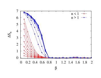
We also explain the importance of the random sign structure. This effect we compare the behavior of the second Rényi entropies $\langle S_{2}(\rho_{A})\rangle$ for $|\Psi_{REM+\textrm{sign}}\rangle$ with $|\Psi_{REM}\rangle$ without random sign. The difference, $\Delta S_{2}$, is found to decrease monotonically as a function of disorder strength. In the low disorder regimes, $\langle S_{2}(\rho_{A})\rangle$ for $|\Psi_{REM}\rangle$ is a constant and thus their difference $\Delta S_{2}$ takes the maximal value. At the values of $t\leq 1/3$, the difference disappears before entering into the MBL phase.

Figure 1: (Color online). (a) Phase diagram for the classical REM model as a function of $\beta$. The spin glass phase transition occurs at $\beta=\sqrt{2\log 2}$. The shaded region between $\sqrt{\log 2/2}$ and $\sqrt{2\log 2}$ has non-Gaussian fluctuation. (b) Schematic phase diagram for the REM wave function in terms of the entanglement entropy showing different scaling behaviors in four different regimes as a function of $\beta$. In the regime (i) $\langle S_{n}\rangle$ is equal to $N_{A}\log 2$ for all $N_{A}$. In the intermediate regime (ii), $\langle S_{2}\rangle$ is sub-extensive but does not saturate to a constant. Regime (iii) is the MBL phase. In this regime, the wavefunction is not localized in the Hilbert space. (iv) is also the MBL phase with the wavefunction localized in Hilbert space.

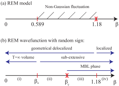
The rest of the paper is organized as follows. In Section II, we explain the construction of a Rokhsar-Kivelson-type wave function which assigns to the amplitude of a quantum many-body state the Gibbs weight of a classical spin glass model (the Random Energy Model) and introduce a random sign structure into it to access represent typical excited states with a finite excitation energy density. In Section III.1 we briefly review the classical random energy model (REM) and interpret the classical spin glass phase transition in it. In the Section III.2 we construct a REM wave function with a random sign structure to mimic a highly excited state for a Hamiltonian with disorder. We will analytically compute the Rényi entropy to show that there is a thermalized regime and a many-body localized phase. In Section IV we calculate the Rényi entropy numerically and find the location of MBL phase transition by finite size scaling. In the Section IV.4 we study the Rényi entropy for the REM wave function without random sign and demonstrate the importance of the sign structure. In the Section V we summarize our results and conclude that there is a MBL phase transition in the REM wave function with random sign structure.

II Rokhsar-Kivelson Model wave functions

In the physics of strongly correlated systems there are many examples in which the properties of a new state of matter can be represented by simple ‘model’ wave functions. The best known examples of such model wave functions include the BCS wave function for the ground state of a superconductor and the Laughlin wave function for the fractional quantum Hall fluid.

II.1 RK-type wave functions

In this paper we will give a description of the MBL states using a particularly simple class of model wave functions with a structure similar to the one proposed by Rokhsar and Kivelson (RK) to capture the physics of the ground states of strongly frustrated quantum antiferromagnets.Rokhsar and Kivelson (1988) In the RK construction the quantum mechanical amplitude of a many-body state is given by a local function of the degrees of freedom, as expressed in the orthonormal basis set $\{|\mathcal{C}\rangle\}$ where $\mathcal{C}$ is the ‘configuration space’. In the RK problem the configuration space is the set of dimer coverings of a 2D lattice. While in the RK case the dimers are a qualitative representation of spin singlets on each bond of the lattice, a picture of this type has been generalized to many other systems, including Kitaev’s Toric Code state,Kitaev (2003) which represents the topological (or deconfined) phase of a $\mathbb{Z}_{2}$ gauge theory.

Since the weights of the RK wave functions are local and positive, they can also be regarded as the Gibbs weights of a related problem in classical statistical mechanics with the same degrees of freedom on the same lattice. Thus if the basis of orthonormal states is the set $\{|\mathcal{C}\rangle\}$, i.e. such that $\langle\mathcal{C}|\mathcal{C}^{\prime}\rangle=\delta_{\mathcal{C},\mathcal{C}^{\prime}}$, the generalized normalized RK states are

$$|\Psi\rangle=\frac{1}{\sqrt{\mathcal{Z}}}\sum_{\{\mathcal{C}\}}e^{-\frac{\beta}{2}E[\mathcal{C}]}|\mathcal{C}\rangle$$ (6)

where

$$\mathcal{Z}=\sum_{\{\mathcal{C}\}}e^{-\beta E[\mathcal{C}]}$$ (7)

Here $E[C]$ and $\mathcal{Z}$ are, respectively, the energy for the classical configuration $\mathcal{C}$ and the partition function for the associated classical problem, and $\beta$ plays the role of the inverse temperature. The original RK wave function is an equal-amplitude superposition of all dimer coverings in $2D$. This wave function can be associated with the partition function for the classical dimer model and is also the ground state of the quantum dimer model at the critical point Rokhsar and Kivelson (1988); Ardonne et al. (2004); Fradkin (2013) (for 2D bipartite lattices) and a $\mathbb{Z}_{2}$ topological stateMoessner and Sondhi (2001) (for non-bipartite lattices). States of these type are exact ground states of a special type of quantum Hamiltonians that are the sum of projection operators and are closely related to classical dynamics.Henley (2004); Castelnovo et al. (2004)

The generalized RK wave function $|\Psi_{REM}\rangle$ inherits many properties from the classical model. For instance, the equal time correlation function of the wave function is the same as the correlation function of the classical model, and the quantum critical point in the wave function corresponds to the classical phase transition at temperature $1/\beta_{c}$.

II.2 Random sign wave function

We want to consider our family of wave functions as representing finite energy density states with the possibility of supporting both ergodic and MBL phases. As we noted above, there exists Hamiltonians constructed by projection operators for which the RK wave functions of the form of Eq.(6) are the exact ground states. However, we should note that its amplitudes are all strictly positive. If the classical Hamiltonian used to generate the RK state only has local interactions, we can show this state must have an area law. This follows from the fact that one can write a Schmidt decomposition of the state where the number of terms is bounded by the number of classical interactions which are broken (See Appendix A for detail). The entanglement properties of these type of states have been discussed in great detail in the case of the quantum dimer model,Furukawa and Misguich (2007); Castelnovo and Chamon (2007); Stéphan et al. (2009) of the associated quantum Lifshitz model,Fradkin and Moore (2006); Hsu et al. (2009); Hsu and Fradkin (2010) and of the Toric Code state.Hamma et al. (2005); Levin and Wen (2006)

To have the potential for ergodic states, then, we must either use a non-local classical Hamiltonian or introduce directly a more rich sign structure into the wave function as done, e.g., in Refs. Grover and Fisher, 2014a, b. While the classical Hamiltonian we are using for the REM model is non-local, it nonetheless supports an area law at low disorder; in fact, at $\beta=0$, the entanglement entropy is zero over any cut. Therefore, we introduce a random sign structure in the wave function giving

$$|\Psi_{REM+\rm{sign}}\rangle=\frac{1}{\sqrt{\mathcal{Z}}}\sum_{\{\mathcal{}C\}}\ s_{\mathcal{C}}\;e^{-\frac{\beta}{2}E[\mathcal{C}]}|\mathcal{C}\rangle,$$ (8)

where $s_{\mathcal{C}}$ is a quenched random sign associated to each configuration $\mathcal{C}$. The average ratio between the number of positive and negative signs is one. A similar construction was discussed in Ref. Khemani et al., 2014, where they showed that the random sign structure can lead to a thermalized phase. In this paper, we will study the MBL phase transition in a RK-wave function with random sign.

III Many body localization phase transition

In this section we will show that the RK wave function with random signs has an ergodic (thermalized) regime and an MBL phase. We begin with a summary of the properties of the classical Random Energy Model whose Boltzmann weights will enter into the structure our wave function.

III.1 The Random Energy Model

The random energy model (REM) is a simple classical model which has a phase transition to a spin glass phase.Derrida (1980) This effectively infinite dimensional model has $2^{N}$ configurations and is the infinite range coupling limit of the Sherrington-Kirkpatrick spin glass model.Sherrington and Kirkpatrick (1975) In the REM model, the energy for each configuration is no longer given by the complicated spin glass Hamiltonian, but rather simply an independent random variable. This random variable has the Gaussian distribution

$$P(E)=(2N\pi)^{-1/2}e^{-\frac{E^{2}}{2N}}.$$ (9)

The number of configurations in the energy interval $[N\epsilon,N(\epsilon+\delta)]$, in expectation, is

$$\langle\mathcal{N}(\epsilon,(\epsilon+\delta))\rangle=\int_{\epsilon}^{\epsilon+\delta}dxe^{Ns(x)}$$ (10)

where

$$s(x)=\log 2-\frac{x^{2}}{2},\qquad\textrm{with}\;x=\frac{E}{N}$$ (11)

In the thermodynamic limit, $N\to\infty$, this expectation value takes the asymptotic form

$$\lim_{N\to\infty}\langle\mathcal{N}(\epsilon,(\epsilon+\delta))\rangle=\exp\{N\ \mbox{max}_{x\in[\epsilon,\epsilon+\delta]}s(x)\}$$ (12)

Notice that $s(x)>0$ only in the interval $x\in[-\epsilon_{*},\epsilon_{*}]$, where $\epsilon_{*}=\sqrt{2\log 2}$. This means that for $\epsilon\in[-\epsilon_{*},\epsilon_{*}]$, $\langle\mathcal{N}(\epsilon)\rangle$ is exponentially large, and the fluctuations are very small. For $\epsilon$ outside the interval $[-\epsilon_{*},\epsilon_{*}]$, $\mathcal{N}(\epsilon)$ is exponentially small.

The partition function for this model is simply given by

$$\mathcal{Z}=\sum_{i=1}^{2^{N}}e^{-\beta E_{i}}=\int dE\;\mathcal{N}(E)\;e^{-\beta E}=\int dx\;e^{N\phi(x)}.$$ (13)

where $\phi(x)$ equals to

$$\phi(x)=\log 2-\frac{x^{2}}{2}-\beta x,$$ (14)

Similar to the calculation for $\langle\mathcal{N}(\epsilon)\rangle$, we can also use the saddle point approximation to calculate the partition function to obtain

$$\mathcal{Z}=\exp\{N\ \mbox{max}[\phi(x)]\}$$ (15)

which is the exact result in the thermodynamic limit, $N\to\infty$. By computing $\phi_{{\rm max}}=\mbox{max}[\phi(x)]$, it is easy to show that the free energy density equals to

$$f(\beta) = -\frac{\log\mathcal{Z}}{\beta N}=-\frac{\phi_{\rm{max}}}{\beta}$$ (16)

$$= \begin{cases}-\frac{\beta}{2}-\frac{\log 2}{\beta}&\beta<\beta_{sg}\\ -(2\log 2)^{1/2}&\beta\geq\beta_{sg}\end{cases}$$

At $\beta_{sg}=\sqrt{2\log 2}$, there is a discontinuity in the second derivative of the free energy density, showing that there is a phase transition at this point, the spin glass transition.

This phase transition can be further studied by computing the inverse participation ratio (IPR), Derrida (1981); Mezard and Montanari (2009)

$$Y_{n}(\beta)\equiv\sum_{i}^{2^{N}}p_{i}^{n}=\frac{\sum_{i}^{2^{N}}e^{-n\beta E_{i}}}{(\sum_{i}^{2^{N}}e^{-\beta E_{i}})^{n}}.$$ (17)

This quantity measures how many configurations effectively contribute to the partition function and measurable quantities. The expectation value for $Y_{2}$ equals to Mezard and Montanari (2009)

$$\langle Y_{2}(\beta)\rangle=\begin{cases}0&\beta<\beta_{sg}\\ 1-\frac{\beta_{sg}}{\beta}&\beta\geq\beta_{sg}\end{cases}$$ (18)

At low temperatures, $\beta>\beta_{sg}$, the participation ratio takes a finite value. This means that the system is completely frozen to $O(1)$ number of configurations and is in a non-ergodic phase. At high temperature, $\beta<\beta_{sg}$, all configurations will contribute to the thermodynamic properties of the system. For instance, in the high temperature limit $\beta\to 0$, the Boltzmann’s measure becomes uniform and the second participation ratio becomes $Y_{2}(\beta\to 0)=2^{-N}$. When $N\to\infty$, $Y_{2}\to 0$. In general, when $\beta<\beta_{sg}$, $Y_{n}$ scales with the system size

$$Y_{n}\sim\mathcal{D}^{-\tau(n)},\qquad\textrm{with}\;\mathcal{D}=2^{N}$$ (19)

From the results on $\log\mathcal{Z}(\beta)$, we can compute the exponent $\tau(n)$ (for $n>1$)

$$\tau(n)=\begin{cases}(n-1)(1-\gamma n),&0\leq\gamma<\frac{1}{n^{2}}\\ n(1-\sqrt{\gamma})^{2},&\frac{1}{n^{2}}<\gamma<1\\ 0,&\gamma>1\end{cases}$$ (20)

where $\gamma=\frac{\beta^{2}}{2\log 2}$. We will use $\tau(n)$ to give a upper bound for the Rényi entropy of the wave function $|\Psi_{REM+\textrm{sign}}\rangle$ later.

Although the REM model is a simple toy model, it has a spin glass phase transition, i.e., it undergoes a localization transition. It also shows a rich structure in the fluctuation of the free energy. According to the results of Ref. Bovier et al., 2002, for the ergodic phase, which occurs for $\beta<\beta_{sg}$, there are two regimes with different fluctuation behavior of the free energy. When $\beta<\sqrt{\log 2/2}$, the fluctuations of the free energy are Gaussian, and satisfy the central limit theorem. When $\beta_{sg}>\beta>\sqrt{\log 2/2}$, there are non-Gaussian fluctuations of the free energy driven by the Poisson process of the extreme values of the random energies. This regime does not satisfy the central limit theorem. The resulting phase diagram of classical REM model is shown in Fig.1 (a).

III.2 Random sign REM wave function

We can now construct a quantum state following the procedure of Eq.(8),

$$|\Psi_{REM}\rangle=\frac{1}{\sqrt{\mathcal{Z}}}\sum_{\{\mathcal{C}\}}e^{-\frac{\beta}{2}E[\mathcal{C}]}|\mathcal{C}\rangle$$ (21)

whose amplitudes are the Boltzmann weights of the classical REM. By further introducing the random sign structure, the wave function takes the form

$$|\Psi_{REM+\textrm{sign}}\rangle=\frac{1}{\sqrt{\mathcal{Z}}}\sum_{\{\mathcal{C}\}}s_{\mathcal{C}}e^{-\frac{\beta}{2}E[\mathcal{C}]}|\mathcal{C}\rangle$$ (22)

Here both $s_{\mathcal{C}}$ and $E[\mathcal{C}]$ are random variables and are independent of each other. The random sign $s_{\mathcal{C}}$ takes the values $\pm 1$ with equal probability over the entire Hilbert space of $2^{N}$ spin configurations.

Before we do any calculations, we can first estimate the scaling behavior of the Rényi entropy for this quantum state in the extreme limits. In this wave function, $\beta$ is a tuning parameter and has the physical meaning of the disorder strength. The random sign structure is used to represent a highly excited quantum state. When there is no disorder, i.e., $\beta=0$, the amplitude for every configuration is the same. At this point, the Rényi entropy for the subsystem $A$ with different Rényi index is equal to the thermal entropy at infinite temperature. Thus this wave function is thermalized, and the entanglement entropies obey a volume law.Grover and Fisher (2014a) As $\beta$ increases, the disorder becomes stronger and the entanglement entropy becomes smaller. The wave function is eventually localized to a small fraction of the configurations as $\beta>\beta_{sg}$. As we already showed in the previous section, since the number of these configurations is only $O(1)$, in this regime the Rényi entropy is bounded by a finite constant.

III.2.1 Nomenclature and thermodynamic limit for scaling

The entanglement entropy $\langle S_{n}\rangle$ at fixed $\beta$ depends on both the subsystem size $N_{A}$ as well as the total system size $N$ and there can be separate functional forms for the scaling of $\langle S_{n}\rangle$ with respect to either of these parameters. While in many physical systems, these scalings coincide, this is not the case in our model and so it is important to be clear about the distinction. Unless otherwise specified, our discussion will always focus on scaling with $N_{A}$ at fixed system size $N$.

For the thermodynamic limit considered in this work, we let both $N_{A}$ and $N$ go to infinity but their ratio $t=N_{A}/N$ to be a finite value. The changes in entanglement scaling we identify then happen at particular values of $t$ for $0\leq t\leq 1/2$ for different values of $\beta$. The MBL phase in our terminology is identified with scaling collapse.

III.2.2 Analytic Bounds

We now analytically compute bounds to the Rényi entropy. Notice that for a disordered system, we need to take a quenched ensemble average of the Rényi entropy,

$$\langle S_{n}(\rho_{A})\rangle=\frac{1}{1-n}\langle\log\mbox{Tr}\rho_{A}^{n}\rangle$$ (23)

In this quenched average the disorder is frozen and does not evolve with time. We mainly focus here on the second Rényi entropy, but the results are easily extended to the other Rényi entropies.

We begin by noting that the quenched average in Eq.(23) is redundant if, in the thermodynamic limit, the system is self-averaging.Buffet (1993) However, this will not always be the case. For brevity, we sometimes will denote $\langle S_{n}(\rho_{A})\rangle\equiv\langle S_{n}\rangle$.

Let us define a bipartition our system of $N$ spins into two subsets (or regions), $A$ and $B$. The reduced density matrix for region $A$ is

$$\rho_{a,a^{\prime}}^{A} = \frac{1}{\mathcal{Z}}\left(\sum_{b}s_{a,b}s_{a^{\prime},b}e^{-\frac{\beta}{2}(E_{a,b}+E_{a^{\prime},b})}\right)|\mathcal{C}_{a}\rangle\otimes\langle\mathcal{C}_{a^{\prime}}|$$ (24)

$$= \frac{\widetilde{\rho}^{A}_{a,a^{\prime}}}{\mathcal{Z}}$$

where $\widetilde{\rho}^{A}_{a,a^{\prime}}$ is the unnormalized reduced density matrix.

For the above reduced density matrix, $\langle S_{n}(\rho_{A})\rangle$ equals to

$$\langle S_{n}(\rho_{A})\rangle=\frac{1}{1-n}\left(\langle\log\mbox{Tr}\widetilde{\rho}_{A}^{n}\rangle-n\langle\log\mathcal{Z}(\beta)\rangle\right)$$ (25)

The second term $\langle\log\mathcal{Z}(\beta)\rangle$ can be calculated by the saddle point approximation and the result is already shown in Eq.(16). However, the first term $\langle\log\mbox{Tr}\widetilde{\rho}_{A}^{n}\rangle$ is hard to obtain analytically. Instead of calculating it directly, we compute a lower bound and upper bound for it.

Lower Bound

: Consider the annealed average

$$S_{n}(\langle\widetilde{\rho}_{A}\rangle)=\frac{1}{1-n}\left(\log\langle\mbox{Tr}\widetilde{\rho}_{A}^{n}\rangle-n\langle\log\mathcal{Z}(\beta)\rangle\right)$$ (26)

which is much easier to compute. By using Jensen’s inequality,Reed and Simon (1981) when $n>1$, it is straightforward to see that the annealed average of the Rényi entropy $S_{n}(\langle\widetilde{\rho}_{A}\rangle)$ provides a lower bound for the quenched average $\langle S_{n}(\rho_{A})\rangle$, i.e.

$$\langle S_{n}(\rho_{A})\rangle\geq S_{n}(\langle\widetilde{\rho}_{A}\rangle)$$ (27)

To obtain the annealed average $S_{2}(\langle\widetilde{\rho}_{A}\rangle)$, we need to calculate $\langle\mbox{Tr}\widetilde{\rho}_{A}^{2}\rangle$. By means of simple manipulations we find

$$\langle\mbox{Tr}\widetilde{\rho}_{A}^{2}\rangle= \sum_{a,a^{\prime}}\langle(\widetilde{\rho}^{A}_{a,a^{\prime}})^{2}\rangle$$

$$= \sum_{a}\langle\left(\widetilde{\rho}_{a,a}^{A}\right)^{2}\rangle+\sum_{a\neq a^{\prime}}\langle\left(\widetilde{\rho}^{A}_{a,a^{\prime}}\right)^{2}\rangle$$

$$= \sum_{a}\langle\Big{(}\sum_{b}e^{-\beta E_{a,b}}\Big{)}^{2}\rangle$$

$$+\sum_{a\neq a^{\prime}}\langle\Big{(}\sum_{b}s_{a,b}s_{a^{\prime},b}e^{-\frac{\beta}{2}(E_{a,b}+E_{a^{\prime},b})}\Big{)}^{2}\rangle$$

$$= 2^{N}e^{2N\beta^{2}}+(2^{N_{B}}-1)2^{N}e^{N\beta^{2}}+(2^{N_{A}}-1)2^{N}e^{N\beta^{2}}$$ (28)

where the last step is derived by using that for a Gaussian distribution $\langle e^{-\alpha E}\rangle=e^{\alpha^{2}N/2}$.

In the thermodynamic limit, when $N_{A}<N$, the annealed average of the second Rényi entropy becomes

$$S_{2}(\langle\widetilde{\rho}_{A}\rangle)=\begin{cases}N_{A}\log 2,&\beta\leq\beta_{1}\\ N(\log 2-\beta^{2}),&\beta>\beta_{1}\end{cases}$$ (29)

where $\beta_{1}=\sqrt{(1-t)\log 2}$ and $t$ is the ratio $N_{A}/N$. The result is plotted in Fig.2 (a), where the black dashed curve is the lower bound for $\langle S_{2}\rangle/S_{T}$ at $t=1/3$. $S_{T}=N_{A}\log 2$ is the thermal entropy for subsystem $N_{A}$ at infinite temperature. Notice that when $\beta\leq\beta_{1}$, since the lower bound $S_{2}(\langle\widetilde{\rho}_{A}\rangle)=S_{T}$, $\langle S_{2}(\rho_{A})\rangle$ must be equal to $N_{A}\log 2$. When $\beta>\sqrt{\log 2}$, $S_{2}(\langle\widetilde{\rho}_{A}\rangle)<0$, this lower bound is replaced by zero and is not useful anymore.

Upper Bound

: It is easy to see that $\mbox{Tr}\rho_{A}^{2}$ can be bounded from below by the second participation ratio of the classical REM. Indeed,

$$\mbox{Tr}\rho_{A}^{2}>\frac{\sum_{a}(\sum_{b}e^{-\beta E_{a,b}})^{2}}{\mathcal{Z}(\beta)^{2}}>\frac{\mathcal{Z}(2\beta)}{\mathcal{Z}(\beta)^{2}}=Y_{2}(\beta)$$ (30)

Thus, an upper bound for the quenched average $\langle S_{2}(\rho_{A})\rangle$ is given by

$$\langle S_{2}(\rho_{A})\rangle<\tau_{2}(\beta)N\log 2$$ (31)

where $\tau_{2}(\beta)$ is defined in Eq.(20). This upper bound puts a constraint on $\langle S_{2}(\rho_{A})\rangle$, showing that when

$$\beta>\beta_{ub}(n=2)=(1-\sqrt{\frac{t}{2}})\sqrt{2\log 2}$$ (32)

then

$$\langle S_{2}(\rho_{A})\rangle<N_{A}\log 2$$ (33)

which is the thermal entropy at infinite temperature. The red solid curve in Fig.2 (a) is the upper bound for $\langle S_{2}\rangle/S_{T}$ at $t=1/3$.

Figure 2: (Color online) (a) The lower and upper bound for $\langle S_{2}\rangle$. The black dashed curve is for the lower bound and the red solid curve is for the upper bound. The system size $N=300$ and the ratio $t=1/3$. (b) The upper bound for $\langle S_{n}\rangle$. The setup is the same as (a).

Figure 3: (Color online) A summary of our knowledge of the phase diagram of $\Psi_{REM+\textrm{sign}}$, based on $\langle S_{n}\rangle$. The dotted black line indicates a bound to the left of which $\langle S_{2}\rangle$ analytically follows the $T=\infty$ volume law (ITV). The dotted red line indicates a bound to the right of which $\langle S_{2}\rangle$ analytically is strictly below the $T=\infty$ volume law. $\beta_{sg}$ indicates analytically the transition to a localized Hilbert space for any $N_{A}/N$ and a guaranteed constant for all $\langle S_{n}\rangle$. The solid purple dots indicate the numerically computed transition points for $\langle S_{2}\rangle$ (the purple line is a fit for the eye). In comparison, the blue dashed line indicates a bound to the right of which $\langle S_{\infty}\rangle$ analytically is strictly less then ITV, and suggests multifractality.

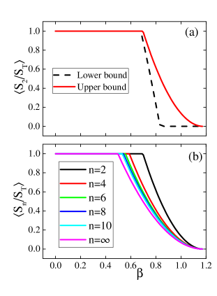
Using a similar approach, we can prove that when $n$ is an even number, $\mbox{Tr}\rho_{A}^{n}\geq Y_{n}(\beta)$, and the quenched averaged $n$th Rényi entropy satisfies

$$\langle S_{n}(\rho_{A})\rangle<\frac{\tau_{n}(\beta)N\log 2}{n-1}$$ (34)

This upper bound indicates that when

$$\beta>\beta_{ub}(n)=(1-\sqrt{\frac{n-1}{n}t})\sqrt{2\log 2}$$ (35)

we obtain the bound

$$\langle S_{n}(\rho_{A})\rangle<N_{A}\log 2$$ (36)

which, again, is the thermal entropy at the infinite temperature. The result for the upper bound is shown in Fig.2 (b). Notice that when $\beta\leq\beta_{ub}(n=\infty)$, the different curves in Fig.2 (b) are overlapping with each other. When $\beta_{ub}(n=\infty)<\beta<\beta_{sg}$, the upper bounds for $\langle S_{n}\rangle$ show different scaling behavior. Combining the upper and lower bounds for different $n$ leads to a regime where the $n=2$ Rényi entropy satisfies a volume law and behaves like a thermal entropy at infinite temperature, but for $n>2$ is strictly below this bound.

Implications from the bounds

: From the above results, we find an upper and lower bound for the Rényi entropy. Here we consider $\langle S_{2}\rangle$ in detail, which thus has the following behaviors

$$\begin{cases}\langle S_{2}\rangle=S_{2}(\langle\widetilde{\rho}_{A}\rangle)=N_{A}\log 2,&\beta\leq\beta_{1}\\ N(\log 2-\beta^{2})<\langle S_{2}\rangle<N_{A}\log 2,&\beta_{2}<\beta<\beta_{sg}\\ \langle S_{2}\rangle<-\log(1-\beta_{sg}/\beta),&\beta>\beta_{sg}\end{cases}$$ (37)

where $\beta_{2}=\beta_{ub}(n=2)=(1-\sqrt{t/2})\sqrt{2\log 2}$.

For $\langle S_{2}\rangle$, there is a regime where $\langle S_{2}\rangle$ satisfies the volume law and equals the thermal entropy at $T=\infty$. When $\beta>\beta_{sg}$, $\langle S_{2}\rangle$ is bounded by a finite constant. A phase transition into the MBL phase is expected to be between $\beta_{1}\leq\beta\leq\beta_{sg}$ . To find the location of the MBL phase transition, we will use scaling collapse in Section IV.

III.3 Localization properties of the wave function

We end this Section with a discussion of the statistical properties of the states $|\Psi_{REM}\rangle$ and $|\Psi_{REM+\textrm{sign}}\rangle$. Given these states, we can define the amplitudes, i.e. their overlap with an eigenstate of the spins $|\mathcal{C}\rangle$. For each state, the square of the amplitude defines a probability distribution for the configuration $\mathcal{C}$ to occur in the state (and hence the random sign does not affect the probability distribution). The resulting probability distribution is thus the same for both states, and it is given by the probability of the configuration $\mathcal{C}$ in the classical REM,

$$P[\mathcal{C}]=|\langle\mathcal{C}|\Psi_{REM}\rangle|^{2}=\frac{1}{\mathcal{Z}}e^{-\beta E[\mathcal{C}]}$$ (38)

Given this probability distribution, we can compute its Shannon-Rényi entropies, which one can immediately see, c.f. Eq.(17), to be the same as the IPR of the classical REM. Hence, the localization of wave function in the Hilbert space can be characterized by the IPR defined in the configuration space. For REM wave function,

$$Y_{n}=\sum_{\{\mathcal{C}\}}|\langle\Psi|\mathcal{C}\rangle|^{2n}=\frac{\sum_{i=1}^{2^{N}}e^{-n\beta E_{i}}}{\left(\sum_{i=1}^{2^{N}}e^{-\beta E_{i}}\right)^{n}}$$ (39)

This is the same as the IPR for the classical REM model defined in Eq.(17). Since $\tau(n)$, defined in Eq.(19), is the multifractal spectrum, given explicitly in Eq.(20), in the regime $0<\beta<\beta_{sg}$, the wave function itself has multifractal behavior. The multifractality of the wave function indicates the pre-freezing behavior before entering into the MBL phase. Similar phenomenon was also observed in Refs.Luca and Scardicchio, 2013; Luitz et al., 2015, where they found that at the MBL phase transition point, the whole wave function is still delocalized in the configuration space.

We can now use the results of the inverse participation ratios of the classical REM summarized in section III.1 to draw conclusions on the degree of localization in the $2^{N}$-dimensional Hilbert space of the $|\Psi_{REM}\rangle$ and $|\Psi_{REM+\textrm{sign}}\rangle$ wave functions. From the results of Section III.1 we find that for $\beta>\beta_{sg}=\sqrt{2\log 2}$ all the inverse participation ratios are finite as $N\to\infty$ and, hence, that the Shannon-Rényi entropies for the wave functions are finite (and are not extensive). Thus, in this regime these wave functions are (exponentially) localized. On the other hand, for $\beta<\beta_{sg}$, the IPRs of the REM vanish exponentially fast as $N\to\infty$, and so do the Shannon-Rényi entropies of the wave functions. In this regime the wave functions are not localized. In this regime the multifractal nature of these wave functions is manifest in the size dependence of their Shannon-Rényi entropies. We should emphasize that, beyond setting the bounds that we have discussed earlier in this section, the knowledge the behavior of the Shannon-Rényi entropies alone yields no information on the scaling of quantum entanglement, which is our main interest.

IV Numerical results on MBL phase transition

In the previous section, we were able to analytically establish the existence of a regime in which the quenched averaged second Rényi entropy $\langle S_{2}\rangle$ is strictly less than ITV scaling, and happens strictly before the localization transition. Nothing prevents this regime from being one in which $\langle S_{2}(N_{A})\rangle$ still scales linearly but at finite $T$; in addition, it doesn’t separate the MBL transition from the localization transition. To establish this, we numerically identify the transition point via scaling collapse. We explicitly construct different disorder samples from the random sign REM wave function and calculate the quenched average $\langle S_{n}\rangle$ with at least 1000 disorder realizations. First, we focus on the $n=2$ case, and then discuss the other values of $n$. As a sanity check, we verify that our numerical results are consistent with the analytical results above at large and small $\beta$.

The following is a summary of our numerical results.

At small $\beta$

: Analytically we anticipate ITV for $n=2$. In Fig. 4, we concretely consider $\beta=0.3$ at $N=30$ with 2000 disorder realizations. We see that it corresponds to the expected $\langle S_{2}\rangle=N_{A}\log 2$.

As $N_{A}\log 2$ is the maximal entanglement entropy for any given realization, for a $T=\infty$ volume law to hold, essentially all but a measure zero fraction of configurations must have this entropy. From the inset of Fig.6b, one can see that the standard deviation of $\langle S_{2}\rangle$ at $\beta=0.3$ is zero showing this is indeed the case. Similar behavior can be observed for $\langle S_{n}\rangle$ with other Rényi indices, where $\langle S_{n}\rangle=N_{A}\log 2$ and $\langle\delta S_{n}\rangle$ is close to zero as $\beta\leq\beta_{*}$.

At large $\beta>\beta_{sg}$

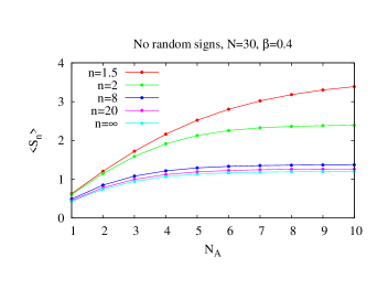
: We find analytically that $\langle S_{n}\rangle$ with $n\geq 2$ is bounded by a finite constant and, hence, in this range the state is in the MBL phase. Note that a constant for small $n$ gives a bound for the entanglement entropy for all larger $m$ as $S_{n}>S_{m}$ if $m>n$. In Fig.4 the numerical results for $\beta=1.5$ are presented, and show that when $N_{A}$ increases, $\langle S_{n}\rangle$ saturates to some constant value. Notice also from the inset of Fig.6b, that as we move deeper into the localized phase, the standard deviation is monotonically decreasing.

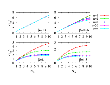
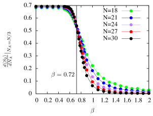
The change from ITV to constant in the entanglement entropy can be seen in Fig.5, which shows $d\langle S_{2}\rangle/dN_{A}$ as a function of $\beta$. As system sizes increases, the slope quickly approaches $\log 2$ for $\beta<0.5$, and approaches $0$ for $\beta>1.2$. The slopes for all 5 values of $N$ start to drop around $\beta=0.6$, which is less than the $\beta_{2}=(1-\sqrt{1/6})\sqrt{2\log 2}\approx 0.6967$ in Eq.(37) for subsystem ratio $t=1/3$ and is consistent with the analytical result.

Figure 4: (Color online) The numerical results for $\langle S_{n}\rangle$ with $n$ from $1$ to $\infty$ at different values of $\beta$. The total system size is $N=30$. Each point in the plot is averaged over 2000 disorder realizations. At $\beta=0.3$, $S_{n}$ shows ITV behavior for all $n$. At $\beta=0.66,1.1$, $\langle S_{n}\rangle$ deviates from the ITV with increasing $\beta$, but the speed at which it moves away depends on its Rényi index. At $\beta=1.5$, $\langle S_{n}\rangle$ is a constant for all $n$.

IV.1 Finite-size scaling

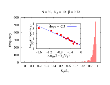
To locate the MBL phase transition, we use both $\langle S_{2}\rangle$ and its standard deviation, $\delta S_{2}$.Kjall et al. (2014); Vosk et al. (2014) For instance, in the bottom inset of Fig. 6, it is shown that when $\beta>0.5$, $\delta S_{2}/S_{T}$ will increase rapidly and reach the maximum value at some $\beta$. Fig. 6 (bottom) shows that the standard deviation at intermediate values of $\beta$ is actually a non-trivial fraction of the maximum thermodynamic entropy. In fact, because of the breakdown in the REM of the Central Limit Theorem, the fluctuation of the Rényi entropy is non-Gaussian. This is seen, for example, in the distribution of $S_{2}/S_{T}$ at $\beta=0.72$ shown in Fig.7, which is peaked around 1 and has a long tail. This long tail has power law scaling behavior shown in the inset of Fig.7, with a power-law exponent between -3 and -2, which implies a well-defined average but an infinite variance in the thermodynamic limit (which is consistent with the peak scaling as $S_{T}$). This may be related to the quantum Griffiths phase found in Ref. Vosk et al., 2014; Agarwal et al., 2015; Potter et al., 2015.

Figure 5: (Color online) $\frac{d\langle S_{2}\rangle}{dN_{A}}$ vs $\beta$ graph at $t=1/3$, where the slopes are obtained from finite differences. As $\beta$ increases, the slopes drop from $\log 2$ towards 0 for all 5 different system sizes.

Figure 6: (Color online). a) Scaling collapse of $\langle S_{2}\rangle/S_{T}$ at $t=1/3$, where $S_{T}=N_{A}\log 2$. It can be noticed that $b$ is very close to 0. b) Scaling collapse of $\delta S_{2}/S_{T}$. The left insets show the original curves. Two scaling collapses give very close $\beta_{c}$ values. Error analysis is only performed on the scaling collapse of $\langle S_{2}\rangle/S_{T}$.

Figure 7: (Color online) The distribution of $S_{2}/S_{T}$ at $\beta=0.72$. The total number of samples is 2000. The number of bins used to make the histogram is 100. The inset shows a log-log plot with a linear fit, which indicates a power law distribution. The number of bins in the log-log scale is 20 for $S_{2}/S_{T}$ from 0 to 1. However, as many of the bins have 0 sample, some points are not included the log-log plot.

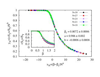
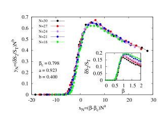
While we can use the peak of $\delta S_{2}$ and the transition of $\langle S_{2}\rangle$ from maximal to zero to locate the phase transition, these quantities scale with system size. We therefore use finite-size scaling to find the MBL phase transition. In the regime of interest, we perform a scaling collapse of the data for the two ratios $\langle S_{2}\rangle/S_{T}$ and $\delta S_{2}/S_{T}$ separately, using scaling functions of the form

$$N^{b}\Phi((\beta-\beta_{c})N^{a})$$ (40)

and determine the form of the scaling functions $\Phi(x)$ numerically. The exponent $b$ is expected to be very close to 0 for $\langle S_{2}\rangle/S_{T}$. When doing the scaling analysis, we find that the quality of the $\langle S_{2}\rangle/S_{T}$ collapse is better than that of the $\delta S_{2}/S_{T}$. Error analysis is only performed on the scaling parameters obtained from $\langle S_{2}\rangle/S_{T}$, although generally the $\delta S_{2}/S_{T}$ collapse yields similar values for $\beta_{c}$.

Notice that this scaling form assumes the existence of only one transition in spite of the fact that we have analytical bounds that show the presence of ITV, constant, and sub-ITV scaling; numerically the latter appears to be neither constant nor linear with subsystem size.

Fig. 6 shows the scaling collapsed for $\langle S_{2}\rangle$ at $t=1/3$. In previous work on MBL phase transition, $\nu\equiv a^{-1}$ in Eq.(40), is the critical exponent for the localization length and is expected to satisfy Harris inequality $\nu\geq 2/d$, where $d$ is the spatial dimension. However REM model is a highly non-local model and $d$ here is equal to infinity, which suggests that there is no bound for $\nu$. To make sure the scaling parameters obtained are truly associated with this transition, one can use them to scale the $\langle S_{n}\rangle/S_{T}$ data following Ref. Luitz et al., 2015. For each $\beta$, we plot $\langle S_{n}\rangle$ vs $N$ as shown in the inset of Fig. 8 , from which one can see that the scaled curves bifurcate smoothly into the two branches depending on $\beta$. Furthermore, Fig. 8 indicate that the system experiences a phase transition rather than a crossover, because of the clear separation of the two branches at large $N$.

Figure 8: (Color online) This graph uses the scaling parameters obtained from Fig. 6 to scale the $\langle S_{2}\rangle/S_{T}$ vs $N$ curves for $\beta$ values ranging from 0 to 2. The scaled graph clearly shows two branches – (1) curves with large $\beta$ flow to low entanglement entropy; (2) curves with small $\beta$ flow to $T=\infty$ entanglement entropy, i.e. $N_{A}\log 2$. The right inset shows the original curves, where each curve corresponds to a different $\beta$.

Figure 9: (Color online) (a) Scaling collapse of $\langle S_{\infty}\rangle/S_{T}$ at $t=1/3$, where $S_{T}=N_{A}\log 2$. It can be noticed that $b$ is very close to 0. (b) Scaling collapse of $\delta S_{\infty}/S_{T}$. The left insets show the original curves. Two scaling collapses give very close $\beta_{c}$ values. Error analysis is only performed on the scaling collapse of $\langle S_{\infty}\rangle/S_{T}$.

Figure 10: (Color online) This graph uses the scaling parameters obtained from Fig. 9 to scale the $\langle S_{\infty}\rangle/S_{T}$ vs $N$ curves for $\beta$ values ranging from 0 to 2. The scaled graph clearly shows two branches – (1) curves with large $\beta$ flow to low entanglement entropy; (2) curves with small $\beta$ flow to $T=\infty$ entanglement entropy, i.e. $N_{A}\log 2$. The right inset shows the original curves, where each curve corresponds to a different $\beta$.

Figure 11: (Color online) $\beta_{c}$ vs $\frac{n-1}{n}$ curve at $t=1/3$. The linear fit line’s slope is $-0.3213\pm 0.0034$, and its y-intercept is $0.9709\pm 0.0023$.

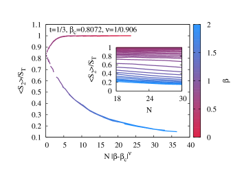
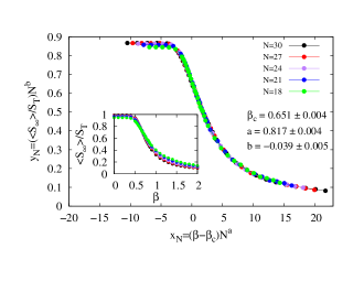
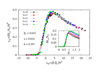
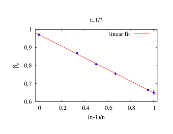
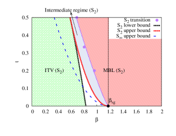
We have also done scaling collapse for $\langle S_{2}\rangle$ with other subsystem ratios. At $t=1/2$, we get $\beta_{c}=0.693$; and at $t=1/5$, we get $\beta_{c}=0.965$. These results are shown as purple dots on Fig. 3. All our collapsing results are summarized in Table 1.

	$t$	$n$	$a$	$b$	$\beta_{c}$
	1/3	1	0.811	0.007	0.970
	1/3	1.5	0.897	0.0093	0.8680
	1/3	2	0.906	−0.0006	0.8072
$\frac{\langle S_{n}\rangle}{S_{T}}$	1/3	3	0.902	0.0095	0.755
	1/3	20	0.8389	−0.025	0.6657
	1/3	$\infty$	0.817	−0.039	0.651
	1/2	2	0.90	−0.070	0.693
	1/5	2	0.766	0.010	0.965
	1/3	1	0.893	0.321	0.983
	1/3	1.5	0.902	0.396	0.861
	1/3	2	0.923	0.400	0.798
$\frac{\delta S_{n}}{S_{T}}$	1/3	3	0.908	0.399	0.753
	1/3	20	0.835	0.383	0.655
	1/3	$\infty$	0.824	0.397	0.643
	1/2	2	0.909	0.090	0.678
	1/5	2	0.856	0.147	0.963

Table 1: Collected scaling collapse data

Based on the above numerical results, we conclude that the MBL transition (both of $\langle S_{2}\rangle$ and all the other $\langle S_{n}\rangle$ (see Sec.IV.3 and Appendix C) happen separately from the localization transition at $\beta_{sg}$. The MBL phase transition is at $\beta_{c}$ and is smaller than $\beta_{sg}$. Between $\beta_{c}$ and $\beta_{sg}$, although it is in the MBL phase, the whole wave function is still delocalized in the Hilbert space. Only when $\beta>\beta_{sg}$, the wave function becomes localized in the Hilbert space and is already deep in the MBL phase.

IV.2 Intermediate regime

According to the scaling collapse in Fig. 6, the MBL phase transition for $\langle S_{2}\rangle$ happens at around $0.8$ at $t=1/3$. From Eq.(32), we also know that when $\beta>0.697$, $\langle S_{2}\rangle<N_{A}\log 2$. This implies that there is an intermediate regime between ITV and MBL phase (regime (ii) in Fig.1 (b)). In this regime, $\langle S_{2}\rangle$ is sub-extensive and the slope

$$0<s(N_{A})=\frac{1}{\log 2}\frac{d\langle S_{2}\rangle}{dN_{A}}<1.$$ (41)

This regime is not a cross-over but sharply defined with non-analyticities in the curve $s(t)$ signaling its beginning. While a combination of our analytical bounds and numerical results can bound the location of this transition, we are not able to numerically pinpoint its location. It is interesting to note, though, that all the curves in Fig. 5 seem to cross at a single point; for $t=1/3$, this point is approximately $\beta=0.72$ which is surprisingly close to the $\beta_{2}$ bound. While we can’t say anything definitive about the value of the $s(N_{A})$ in the intermediate regime, Fig. 5 shows only two plateaus suggesting that the $s(N_{A})$ in this intermediate regime is not constant. Instead we conjecture that the slope changes continuously as a function of $N_{A}$ in this regime in a nonlinear way. This means that this regime is non-thermal and doesn’t correspond to a thermal density matrix at any temperature. It is not clear whether to call this regime a separate phase, particularly as the data collapse on $\langle S_{2}\rangle/S_{T}$ and $\delta S_{2}/S_{T}$ only identify a single transition.

IV.3 Multifractality of the Rényi entanglement entropies

While we have identified transitions in $\langle S_{2}\rangle$, we can also consider $\langle S_{n}\rangle$ for $n\neq 2$. The analytical bounds (Fig.2) show that there is a regime where $S_{2}$ is still ITV where $S_{\infty}$ scales at a rate less then ITV. We can also use scaling collapse to identify the MBL phase transition in $\langle S_{n}\rangle$; for example, see Fig. 9 and 10. More scaling collapse graphs with different $n$ and subsystem ratio $t$ can be found in Appendix C. We summarize the $N_{A}/N=1/3$ results for various $n$ in Fig.11, from which one can clearly see the transition depends on $n$. We attribute this as a sign of multifractal behavior similar to the multifractal behavior found in the critical wave function of the Anderson localization phase transition point. Wegner (1980) In the Anderson localization problem it is known that multifractality is a feature of the wave function for the mobility edge.Wegner (1980) It is not known if this is also the case in MBL or if there is a multifractal phase. From our data we cannot at present make a definitive determination. It is interesting to note that $\beta_{c}(n)$ is linearly proportional to $(n-1)/n.$ The phase transition point $\beta_{c}$ for von Neumann entropy is $0.97$ and we identify this as the true MBL transition.

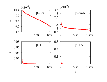
We can understand the different scaling behavior of $\langle S_{n}\rangle$ by considering the entanglement spectrum. Fig.12 is the distribution of eigenvalue $\lambda$ of $\rho_{A}$ for a randomly chosen disorder configuration at different $\beta$. When $\beta=0.3$, $\lambda$ forms a continuous band around $0.001$ which is approximately equal to $1/2^{N_{A}}$. While for $\beta=0.66,1.1$ and $1.5$, there is an obvious gap between the lower continuous band and the other higher eigenvalues. The entanglement gap increases as $\beta$ increases.

This inspires us to write down a simplified two-level model for entanglement spectrum which includes a flat band and a single $\lambda_{max}$. If we assume that $\langle S_{n}\rangle$ is approximately equal to its upper bound in Eq.(34), by using $S_{n=\infty}=-\log\lambda_{max}$, we have

$$\lambda_{max}=2^{-(1-\frac{\beta}{\sqrt{2\log 2}})^{2}N}$$ (42)

All the other $\lambda_{1}\approx 1/2^{N_{A}}$ and there is a gap between $\lambda_{1}$ and $\lambda_{max}$. This toy model exhibits the multifractal behavior described above with a transition to constant entanglement slope that scales with $n>2$. The transition in this simplified model is direct from ITV to constant; to capture our intermediate regime, the single $\lambda_{max}$ can be replaced by a finite number $\lambda_{i}$ with each of them are separated by a finite gap. Also the lower flat band can be replaced a continuous band with more complicated band structure. These additional ingredients are required to have an intermediate regime with sub ITV as well as accurately finding the constant $n=1$ von Neumann entropy.

Figure 12: (Color online) Entanglement spectrum for one randomly chosen disorder configuration at $\beta=0.3,0.66,1.1$ and $1.5$, with $N=30$, $N_{A}=10$. The gaps in the entanglement spectrum become evident when $\beta$ gets larger.

IV.4 The random sign structure in the wave function

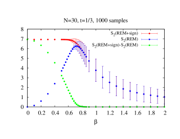
We have introduced a random sign structure to convert our ground state wave function into one at finite energy density. While for any strictly positive wave function, the introduction of random signs can only increase the entanglement entropy, it is interesting to ask what effect, if any, the random sign has here. This requires computing the Rényi entropy $\langle S_{n}(\rho_{A}^{\prime})\rangle$ for the REM wave function without the random sign $|\Psi_{REM}\rangle$. Different from $|\Psi_{REM+\textrm{sign}}\rangle$, the Rényi entropy for $|\Psi_{REM}\rangle$ is not a monotonic function with $\beta$ and has more complicated scaling behavior. In fact $|\Psi_{REM}\rangle$ has zero entanglement entropy at both $\beta=0$ and $\beta\rightarrow\infty$. It is interesting to note that while $\langle S_{2}(\rho_{A})\rangle$ and $\langle S_{2}(\rho_{A}^{\prime})\rangle$ have long tails and infinite variance in the thermodynamic limit at intermediate $\beta$, their difference $\Delta S_{2}=\langle S_{2}(\rho_{A})\rangle-\langle S_{2}(\rho^{\prime}_{A})\rangle$ appears to have finite variance (as shown in Fig. 13).

Figure 13: (Color online) $\langle S_{2}\rangle$ of REM+sign and REM, and their difference. The 1000 disorder configurations are the same for REM+sign and REM. Error bars here represent standard deviations. The difference of the $\langle S_{2}\rangle$ has well bounded variance for all $\beta$.

Since the quenched average $\langle S_{2}(\rho_{A}^{\prime})\rangle$ is hard to access analytically, we can compute a lower bound via Eq.(26) using Jensen’s inequalityReed and Simon (1981) (see Appendix B for details). We find that if $t<1/3$, there is a region $\sqrt{2t\log 2}\leq\beta\leq\sqrt{(1-t)\log 2}$ where $|\Psi_{REM}\rangle$ has ITV entanglement. As this is the maximal allowed value, it then directly follows that there is no difference between $\langle S^{\prime}_{2}\rangle$ and $\langle S_{2}\rangle$ due to the introduction of signs.

Moreover, we conjecture that $\Delta S_{2}$ decreases monotonically as a function of $\beta$. This is consistent with the numerical results shown in Fig.14. Following from this conjecture, we would have that $\Delta S_{2}=0$ for all $\beta\geq\sqrt{2t\log 2}$ and $t<1/3$. This is because, for all $t<1/3$ both models show ITV between $\beta=\sqrt{2t\log 2}$ and $\sqrt{(1-t)\log 2}$ and hence $\Delta S_{2}=0$. The regions B, C, D in Fig. 15 denote where $|\Psi_{REM}\rangle$ and $|\Psi_{REM+\textrm{sign}}\rangle$ have the same $\langle S_{2}\rangle$.

Figure 14: (Color online) Difference of $\langle S_{n}\rangle$ between REM+sign and REM for $n=0.1,\ldots,0.9$ in $0.1$ steps (triangles), and for $n=1.5$, $n=2,\ldots,20$, and $\infty$ (full circles), at $N=30$ and $N_{A}=10$. The number of disorder configurations is 2000. The random configurations are not the same for REM+sign and REM.

Figure 15: (Color online) Different behaviors of $\Delta S_{2}=\langle S_{2}(REM+\textrm{sign})\rangle-\langle S_{2}(REM)\rangle$ on the $t$ vs $\beta$ graph. Region A represents the area where $\langle S_{2}(REM+\textrm{sign})\rangle$ follows ITV and $\langle S_{2}(REM)\rangle$ is a constant, so $\Delta S_{2}$ obeys ITV. Region B represents the area where $\langle S_{2}(REM+\textrm{sign})\rangle$ and $\langle S_{2}(REM)\rangle$ are both ITV, and $\Delta S_{2}$ is zero. As a result, $\Delta S_{2}$ is also zero in Region C based on the monotonicity argument. In Region D, both $\langle S_{2}(REM+\textrm{sign})\rangle$ and $\langle S_{2}(REM)\rangle$ are localized in Hilbert space and $\Delta S_{2}$ is zero. We do not have enough information to determine the behavior $\Delta S_{2}$ in Region E.

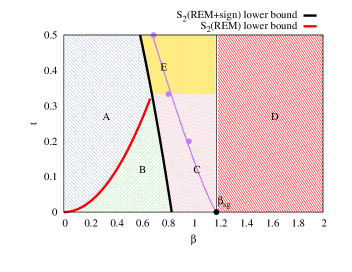
Having identified regimes where the introduction of random signs doesn’t affect the entanglement entropy, we also identify regimes where the entanglement entropy can be shown to be different. When $\beta=0$, $|\Psi_{REM}\rangle$ is a constant (actually a product state) whereas $|\Psi_{REM+\textrm{sign}}\rangle$ is a volume law. We can argue that this extends to larger $\beta$. Defining $X=\mbox{Tr}\widetilde{\rho}_{A}^{2}$ and $Y=\mbox{Tr}(\widetilde{\rho}_{A}^{\prime})^{2}$, where $\widetilde{\rho}_{A}$ is the unnormalized reduced density matrix, we have

$$\langle\log\frac{X}{Y}\rangle\leq\log\langle\frac{X}{Y}\rangle\leq\log\frac{\langle X\rangle}{\langle Y\rangle}$$ (43)

where the second inequality, while not true in general, appears to be numerical validated in our case. In the thermodynamic limit, $\log\frac{\langle X\rangle}{\langle Y\rangle}$ can be directly computed (see Eq.(28) and Eq.(47)). We find that when $t<1/3$ and $\beta\leq\sqrt{2t\log 2}$, $\log\frac{\langle X\rangle}{\langle Y\rangle}=0$. In this region, $\langle S_{2}\rangle$ for $|\Psi_{REM+\textrm{sign}}\rangle$ continues growing as volume while $|\Psi_{REM}\rangle$ stays constant, indicating that the random sign structure can thermalize the wave function and is responsible for the volume law scaling behavior. Fig. 16 is the numerical result for $\langle S_{n}^{\prime}\rangle$ at $\beta=0.4$. We can see that when $n\geq 2$, they all saturate to a constant. This region is highlighted in blue on Fig. 15 and marks a region where the models differ maximally.

Finally, we note that $\Delta S_{n}$ can be numerically computed. Fig.14 is $\Delta S_{n}$ for $N=30$ and $N_{A}=10$. We find that for all $n$, $\Delta S_{n}=0$ when $\beta>0.8$. This result, while only for $N=30$ and so not absent finite-size effects happens to be at the location of the $\langle S_{2}\rangle$ MBL phase transition.

Figure 16: (Color online) The numerical results for $\langle S_{n}^{\prime}\rangle$ without random sign with $n$ from $1.5$ to $\infty$ at $\beta=0.4$. The total system size is $N=30$. Each point in the plot is the average of 2000 disorder realizations.

V Conclusions

We have studied the many-body localization phase transition in a class of many-body wave functions. We focused our analysis in a class of wave functions, $|\Psi_{REM}\rangle$, whose amplitudes are the Boltzmann weights of a classical spin glass model in infinite dimension, the Random Energy Model. In order to mimic the structure of wave functions of highly excited states with a finite excitation energy density we considered another class of states, $|\Psi_{REM+\textrm{signs}}\rangle$, whose amplitudes are obtained by multiplying the amplitudes of $|\Psi_{REM}\rangle$ by a random sign for each configuration. We studied the MBL problem in the $|\Psi_{REM+\textrm{signs}}\rangle$ wave function, for different regime of the parameter $\beta$, by using both analytical and numerical approaches.

We showed that there is a direct phase transition into the MBL phase. Here we assume that the MBL phase is characterized that the entanglement entropies, as a function of the size of the observed region $N_{A}$, scale to a constant value, a feature that we observed explicitly for large enough values of $\beta$. The location of the phase transition point is identified by scaling collapse of Rényi entropy and its standard deviation. In the thermalized regime, there is a regime where the Rényi entropies with different Rényi index all equal to the thermal entropy $S_{T}$ at $T=\infty$. When $\beta>\beta_{c}$, the system enters into the MBL phase where the entanglement entropy is sub-extensive. The MBL phase transition point $\beta_{c}$ is smaller than $\beta_{sg}$ and this suggests that the MBL phase transition and the classical spin glass phase transition are different. Upon entering the MBL phase, the random sign structure is not important any more and $\langle\Delta S_{n}\rangle$ between $|\Psi_{REM+\textrm{sign}}\rangle$ and $|\Psi_{REM}\rangle$ is zero. For $\beta>\beta_{sg}$, the wave function is deep inside the MBL phase and only $O(1)$ number of the configurations in the REM wave function contributes significantly to the statistical average. The Rényi entropy in this regime will reduce to a finite constant. We find that close to the phase transition point $\beta_{c}$, the fluctuation of Rényi entropy is strong in the finite size system. In this regime, Rényi entropies with different Rényi index show different scaling behavior and are similar to the multifractal behavior observed at the Anderson localization phase transition point. Moreover, $\langle S_{n}\rangle$ has a phase transition at different $\beta_{c}$. Finally we note that we have refrained ourselves from performing the same extensive studies for the wave function without random signs, $|\Psi_{REM}\rangle$. While we have evidence that this wave function too has a thermalized regime, since it has only strictly positive amplitudes we do not expect it to provide an useful description of the MBL problem. Nevertheless it may be useful to investigate its properties in a separate publication.

Note added in the proof: After this work was accepted for publication we became aware of the recent independent work of Yang, Chamon, Hamma and MuccioloYang et al. (2015) who have also discussed the spectrum of the reduced density matrix in several models, including the wave functions discussed in this work.

Appendix A Entanglement entropy for the RK-wave function with classical local Hamiltonian

For the RK-wave function defined in Eq.(6), if the related classical model has a local Hamiltonian, the entanglement entropy satisfies the area law. This scaling behavior only relies on the property of the RK state and does not depend on whether the quantum model is critical or not. Here, we will briefly review the calculation following Ref.Stéphan et al., 2012.

For the RK state with a classical local Hamiltonian, after partitioning the system into two parts A and B, it can be approximately written in this way,

$$|\Psi_{0}\rangle=\sum_{\Gamma}\lambda_{\Gamma}|\Psi_{A}(\Gamma)\rangle|\Psi_{B}(\Gamma)\rangle$$ (44)

where $\Psi_{A}(\Gamma)$ and $\Psi_{B}(\Gamma)$ are the RK wave functions defined in region A and region B with the same boundary configuration $\Gamma$

$$|\Psi_{A}(\Gamma)\rangle=\sum_{A}\frac{e^{-\frac{\beta}{2}H_{A}(\Gamma)}}{\sqrt{\mathcal{Z}_{A}(\Gamma)}}|c_{A}(\Gamma)\rangle$$

$$|\Psi_{B}(\Gamma)\rangle=\sum_{B}\frac{e^{-\frac{\beta}{2}H_{B}(\Gamma)}}{\sqrt{\mathcal{Z}_{B}(\Gamma)}}|c_{B}(\Gamma)\rangle$$ (45)

When $\Gamma\neq\Gamma^{\prime}$, they satisfy $\langle\Psi_{A}(\Gamma)|\Psi_{A}(\Gamma^{\prime})\rangle=0$ and $\langle\Psi_{B}(\Gamma)|\Psi_{B}(\Gamma^{\prime})\rangle=0$. The summation in Eq.(44) is the sum over all possible boundary configurations along the cut and $\lambda_{\Gamma}=\sqrt{\mathcal{Z}_{A}(\Gamma)}\sqrt{\mathcal{Z}_{B}(\Gamma)}/\sqrt{\mathcal{Z}}$.

Thus Eq. (44) is the Schmidt decomposition of the wave function, the reduced density matrix in regime A is

$$\rho_{A}=\sum_{\Gamma}\lambda_{\Gamma}^{2}|\Psi_{A}(\Gamma)\rangle\langle\Psi_{A}(\Gamma)|$$ (46)

Since the dimension of $\rho_{A}$ only depends on the dimension of the Hilbert space along the boundary, the entanglement entropy should satisfy the area law.

Appendix B Lower bound for $\langle S_{2}(\rho_{A}^{\prime})\rangle$

For the REM wave function without random sign, the quenched average $\langle S_{2}(\rho_{A}^{\prime})\rangle$ is hard to access analytically, instead we calculate the annealed average $S_{2}(\langle\rho_{A}^{\prime}\rangle)$ defined in Eq.(26), which gives the lower bound for $\langle S^{\prime}_{2}\rangle$. To obtain $S_{2}(\langle\rho_{A}^{\prime}\rangle)$, we need to know $\langle\mbox{Tr}(\widetilde{\rho}_{A}^{\prime})^{2}\rangle$ first, where $\widetilde{\rho}_{A}^{\prime}$ is the unnormalized reduced density matrix.

$$\langle\mbox{Tr}(\widetilde{\rho}_{A}^{\prime})^{2}\rangle= 2^{N}e^{2N\beta^{2}}+(2^{N_{B}}-1)2^{N}e^{N\beta^{2}}$$

$$+(2^{N_{A}}-1) 2^{N}e^{N\beta^{2}}+(2^{N_{A}}-1)(2^{N_{B}}-1)2^{N}e^{\frac{N\beta^{2}}{2}}$$ (47)

This gives $S_{2}\langle(\rho_{A}^{\prime})\rangle$ in the thermodynamic limit. When $0<t\leq 1/3$, there are three regimes,

$$S_{2}(\langle{\rho}_{A}^{\prime}\rangle)=\begin{cases}\frac{\beta^{2}N}{2},&\beta\leq\sqrt{2t\log 2}\\ N_{A}\log 2,&\sqrt{2t\log 2}<\beta\leq\sqrt{(1-t)\log 2}\\ N(\log 2-\beta^{2}),&\beta>\sqrt{(1-t)\log 2}\end{cases}$$ (48)

When $1/3<t<1/2$, there are two regimes

$$S_{2}(\langle{\rho}_{A}^{\prime}\rangle)=\begin{cases}\frac{\beta^{2}N}{2},&\beta\leq\sqrt{2\log 2/3}\\ N(\log 2-\beta^{2}),&\beta>\sqrt{2\log 2/3}\end{cases}$$ (49)

References

- Bombelli et al. (1986) L. Bombelli, R. K. Koul, J. Lee, and R. D. Sorkin, Phys. Rev. D 34, 373 (1986).
- Srednicki (1994) M. Srednicki, Phys. Rev. E 50, 888 (1994).
- Eisert et al. (2010) J. Eisert, M. Cramer, and M. B. Plenio, Rev. Mod. Phys. 82, 277 (2010).
- Basko et al. (2006) D. M. Basko, I. L. Aleiner, and B. L. Altshuler, Ann. Phys. 321, 1126 (2006).
- Oganesyan and Huse (2007) V. Oganesyan and D. A. Huse, Phys. Rev. B 75, 155111 (2007).
- Pal and Huse (2010) A. Pal and D. A. Huse, Phys.Rev.B 82, 174411 (2010).
- Anderson (1958) P. W. Anderson, Phys. Rev. 109, 1492 (1958).
- Serbyn et al. (2013) M. Serbyn, Z. Papic, and D. A. Abanin, Phys. Rev. Lett. 110, 260601 (2013).
- Huse and Oganesyan (2014) D. A. Huse and V. Oganesyan, Phys. Rev. B 90, 174202 (2014).
- Imbrie (2014) J. Z. Imbrie, “On Many-Body Localization for Quantum Spin Chains,” (2014), arXiv:1403.7837 .
- Ros et al. (2015) V. Ros, M. Müller, and A. Scardicchio, Nuclear Physics B 891, 420 (2015).
- Chandran et al. (2015) A. Chandran, I. H. Kim, G. Vidal, and D. A. Abanin, Phys. Rev. B 91, 085425 (2015).
- Nandkishore and Huse (2015) R. Nandkishore and D. A. Huse, Annual Review of Condensed Matter Physics 6, 15 (2015).
- Monthus and Garel (2010) C. Monthus and T. Garel, Phys. Rev. B 81, 134202 (2010).
- Canovi et al. (2011) E. Canovi, D. Rossini, R. Fazio, G. E. Santoro, and A. Silva, Phys. Rev. B 83, 094431 (2011).
- Morong and DeMarco (2015) W. Morong and B. DeMarco, Phys. Rev. A 92, 023625 (2015).
- Rokhsar and Kivelson (1988) D. S. Rokhsar and S. A. Kivelson, Phys. Rev. Lett. 61, 2376 (1988).
- Ardonne et al. (2004) E. Ardonne, P. Fendley, and E. Fradkin, Annals Phys. 310, 493 (2004).
- Fradkin (2013) E. Fradkin, Field Theories of Condensed Matter Systems (Cambridge University Press, Cambridge, UK, 2013).
- Derrida (1980) B. Derrida, Phys. Rev. Lett. 45, 79 (1980).
- Grover and Fisher (2014a) T. Grover and M. P. A. Fisher, J. Stat. Mech. , P10010 (2014a).
- Grover and Fisher (2014b) T. Grover and M. P. A. Fisher, “Entanglement and the Sign Structure of Quantum States,” (2014b), arXiv:1412.3534 .
- Khemani et al. (2015) V. Khemani, F. Pollmann, and S. Sondhi, “Obtaining highly-excited eigenstates of many-body localized Hamiltonians by the density matrix renormalization group,” (2015), arXiv:1509.00483 .
- Yu et al. (2015) X. Yu, D. Pekker, and B. K. Clark, “Finding matrix product state representations of highly-excited eigenstates of many-body localized Hamiltonians,” (2015), arXiv:1509.01244 .
- Laumann et al. (2014) C. R. Laumann, A. Pal, and A. Scardicchio, Phys. Rev. Lett. 113, 200405 (2014).
- Bauer and Nayak (2013) B. Bauer and C. Nayak, Journal of Statistical Mechanics: Theory and Experiment 9, 5 (2013).
- Thouless (1974) D. J. Thouless, Physics Reports 13, 93 (1974).
- Evers and Mirlin (2008) F. Evers and A. Mirlin, Rev. Mod. Phys. 80, 1355 (2008).
- Wegner (1980) F. Wegner, Zeitschrift für Physik B Condensed Matter 36, 209 (1980).
- de C. Chamon et al. (1996) C. de C. Chamon, Mudry, and X. G. Wen, Phys. Rev. Lett 77, 4194 (1996).
- Castillo et al. (1997) H. E. Castillo, C. C. Chamon, E. Fradkin, P. M. Goldbart, and C. Mudry, Phys. Rev. B 56, 10668 (1997).
- Gruzberg et al. (2011) I. A. Gruzberg, A. W. W. Ludwig, A. D. Mirlin, and M. R. Zirnbauer, Phys. Rev. Lett 107, 086403 (2011).
- Kravtsov et al. (2015) V. E. Kravtsov, I. M. Khaymovich, E. Cuevas, and M. Amini, “A random matrix model with two localization transitions,” (2015), arXiv:1508.01714 .
- Halsey et al. (1986) T. C. Halsey, T. Jensen, L. Kadanoff, I. Procaccia, and B. Shraiman, Phys. Rev. A 33, 114 (1986).
- Jensen et al. (1987) M. H. Jensen, L. Kadanoff, and I. Procaccia, Phys. Rev. A 36, 1409 (1987).
- Jia et al. (2008) X. Jia, A. R. Subramaniam, I. A. Gruzberg, and S. Chakravarty, Phys. Rev. B 77, 014208 (2008).
- Chakravarty (2010) S. Chakravarty, Int. J. Mod. Phys. B. 24, 1823 (2010).
- Chen et al. (2012) X. Chen, B. Hsu, T. L. Hughes, and E. Fradkin, Phys. Rev. B 86, 134201 (2012).
- Luitz et al. (2014) D. J. Luitz, F. Alet, and N. Laflorencie, Phys. Rev. Lett. 112, 057203 (2014).
- Torres-Herrera and Santos (2015) E. J. Torres-Herrera and L. F. Santos, Phys. Rev. B 92, 014208 (2015).
- Vasseur and Moore (2015) R. Vasseur and J. E. Moore, Phys. Rev. B 92, 054203 (2015).
- Kjall et al. (2014) J. A. Kjall, J. H. Bardarson, and F. Pollmann, Phys. Rev. Lett. 113, 107204 (2014).
- Vosk et al. (2014) R. Vosk, D. A. Huse, and E. Altman, Phys. Rev. X 5, 031032 (2014).
- Luca and Scardicchio (2013) A. D. Luca and A. Scardicchio, Europhys. Lett. 101, 37003 (2013).
- Luitz et al. (2015) D. J. Luitz, N. Laflorencie, and F. Alet, Phys. Rev. B 91, 081103 (2015).
- Kitaev (2003) A. Y. Kitaev, Annals of Physics 303, 2 (2003).
- Moessner and Sondhi (2001) R. Moessner and S. L. Sondhi, Phys. Rev. Lett. 86, 1881 (2001).
- Henley (2004) C. Henley, Journal of Physics: Condensed Matter 16, S891 (2004).
- Castelnovo et al. (2004) C. Castelnovo, C. Chamon, C. Mudry, and P. Pujol, Annals of Physics 318, 316 (2004).
- Furukawa and Misguich (2007) S. Furukawa and G. Misguich, Phys. Rev. B 75, 214407 (2007).
- Castelnovo and Chamon (2007) C. Castelnovo and C. Chamon, Phys. Rev. B 76, 184442 (2007).
- Stéphan et al. (2009) J. M. Stéphan, S. Furukawa, G. Misguich, and V. Pasquier, Phys. Rev. B 80, 184421 (2009).
- Fradkin and Moore (2006) E. Fradkin and J. Moore, Phys. Rev. Lett. 97, 050404 (2006).
- Hsu et al. (2009) B. Hsu, M. Mulligan, E. Fradkin, and E.-A. Kim, Phys. Rev. B 79, 115421 (2009).
- Hsu and Fradkin (2010) B. Hsu and E. Fradkin, J. Stat. Mech. P09004 (2010).
- Hamma et al. (2005) A. Hamma, R. Ionicioiu, and P. Zanardi, Physics Letters A 337, 22 (2005).
- Levin and Wen (2006) M. Levin and X.-G. Wen, Phys. Rev. Lett. 96, 110405 (2006).
- Khemani et al. (2014) V. Khemani, A. Chandran, H. Kim, and S. L. Sondhi, Phys. Rev. E 90, 052133 (2014).
- Sherrington and Kirkpatrick (1975) D. Sherrington and S. Kirkpatrick, Phys. Rev. Lett. 35, 1792 (1975).
- Derrida (1981) B. Derrida, Phys. Rev. B 24, 2613 (1981).
- Mezard and Montanari (2009) M. Mezard and A. Montanari, Information, Physics, and Computation (Oxford University press, Oxford, UK, 2009).
- Bovier et al. (2002) A. Bovier, I. Kurkova, and M. Lowe, Ann. Prob. 30, 605 (2002).
- Buffet (1993) E. Buffet, J. Phys. A 26, 1823 (1993).
- Reed and Simon (1981) M. Reed and B. Simon, I: Functional Analysis, revised ed., Methods of Modern Mathematical Physics (Academic Press, London, UK, 1981).
- Agarwal et al. (2015) K. Agarwal, S. Gopalakrishnan, M. Knap, M. Mueller, and E. Demler, Phys. Rev. Lett. 114, 160401 (2015).
- Potter et al. (2015) A. C. Potter, R. Vasseur, and S. A. Parameswaran, Phys. Rev. X 5, 031033 (2015).
- Yang et al. (2015) Z.-C. Yang, C. Chamon, A. Hamma, and E. R. Mucciolo, “Two-component Structure in the Entanglement Spectrum of Highly Excited States,” (2015), arXiv:1506.01714 .
- Stéphan et al. (2012) J. M. Stéphan, G. Misguich, and V. Pasquier, JSTAT-J. Statist. Mech.: Theor. Exp. 2012, P02003 (2012).