The role of the number of degrees of freedom and chaos in macroscopic irreversibility

Abstract

This article aims at revisiting, with the aid of simple and neat numerical examples, some of the basic features of macroscopic irreversibility, and, thus, of the mechanical foundation of the second principle of thermodynamics as drawn by Boltzmann. Emphasis will be put on the fact that, in systems characterized by a very large number of degrees of freedom, irreversibility is already manifest at a single-trajectory level for the vast majority of the far-from-equilibrium initial conditions – a property often referred to as typicality. We also discuss the importance of the interaction among the microscopic constituents of the system and the irrelevance of chaos to irreversibility, showing that the same irreversible behaviours can be observed both in chaotic and non-chaotic systems.

1 Introduction

Everyday experience demonstrates that many natural processes are intrinsically irreversible at the macroscopic level. Think of a gas initially confined by a septum in one half of a container, that spontaneously fills the whole available volume as soon as the separator is removed. Or, closer to daily experience, consider the evolution of an ink drop into water [1]. We would be astounded and incredulous while observing the reverse processes to occur spontaneously: a gas self-segregating in one half of the container, or an ink drop emerging from a water-and-ink mixture. In thermodynamics, the second principle amounts to a formalization of this state of “incredulity”. From Newtonian (and quantum) mechanics, we know that at the microscopic level the dynamics is reversible. How can we reconcile macroscopic irreversibility with microscopic reversibility of the dynamics ruling the elementary constituents of macroscopic bodies?

A solution to this riddle was proposed more than 140 years ago, when Boltzmann laid down the foundation of statistical mechanics. At the beginning, Boltzmann’s ideas on macroscopic irreversibility elicited a heated debate mainly due to the recurrence paradox, formulated by Zermelo, and the reversibility paradox by Loschmidt (a detailed discussion on the historical and conceptual aspects of the Boltzmann’s theory can be found in Refs. [2, 3]). In spite of several rigorous mathematical results [2, 4] supporting, with a clear physical interpretation (at least for many scientists, including the authors of this paper), the coherence of the scenario proposed by Boltzmann, irreversibility still remains a somehow misinterpreted and controversial issue, even among researchers in the field. The reader may appreciate some of the opinions from the comments [5] to a paper by Lebowitz on Boltzmann’s “time arrow”  [1].

According to Boltzmann, irreversibility is well defined only for systems with a very large number of degrees of freedom. It should be observed in the vast majority of the individual realizations of a macroscopic system starting far from equilibrium: “vast majority” is usually referred to as typicality in the literature [6, 7] (see next section for further details). Hence, there is no need to repeat the experiment many times to understand that the free-gas expansion or the spreading of an ink drop in the water are irreversible processes, a single observation is enough. Conversely, for some authors irreversibility can only be properly defined through the use of ensembles. Also, there is not general agreement on the fact that irreversibility is an emergent property when the number of degrees of freedom becomes (sufficiently) large. For instance, Prigogine and his school claim that Irreversibility is either true on all levels or on none: it cannot emerge as if out of nothing, on going from one level to another [8]. For others, irreversibility results from (microscopic) chaotic dynamics, or, it is a mere consequence of the interaction with the external environment.

Likely due to this maze of different opinions, often there is a persistence of confusing and conflicting ideas about macroscopic irreversibility in spite of clear discussions of the subject in the recent past [1, 9, 10].

This article aims at supplementing some aspects of Boltzmann’s explanation of macroscopic irreversibility which are often sources of misinterpretation with simple and neat numerical examples. In particular, the article focuses on the behavior of macroscopic observables that can be measured in laboratory experiments. Boltzmann’s solution to the reversibility and recurrence paradoxes will be mainly left aside as it already widely discussed in the literature (see, e.g., [11, 12]). Instead, emphasis will be put on the fact that irreversibility is a property of the single realization of a macroscopic system in which an important role is played by the (even very weak) interaction among its elementary constituents. In fact, although irreversible behavior can be manifest also in systems of non-interacting units (see Ref. [13] for a pedagogical presentation of irreversibility in the case of non-interacting gas free expansion), in the absence of interactions single-particle and ensemble properties trivially coincide leading to some ambiguity in the interpretation of irreversibility. Finally, to stress the generality of the ideas, simple models, which can be studied by standard simulation techniques, will be considered. In particular, the comparison between chaotic and non-chaotic systems will underline the irrelevance of chaos to irreversibility.

The paper is organized as follows. In Section 2 we briefly survey the conceptual aspects of Boltzmann’s approach, and discuss the entropy, the use of ensembles and the role of chaos. Moreover we present some explicit calculations performed in a Markovian model introduced by P. and T. Ehrenfest [14]. In Sect. 3, we consider numerical examples of macroscopic irreversible behaviors by studying deterministic systems involving particles which collide with a moving wall. In section 4, we discuss a numerical experiment conceptually alike to the irreversible mixing of an ink drop into water. Section 5 summarizes the main aspects of our understanding of macroscopic irreversibility on the light of Boltzmann’s ideas.

2 Basic facts on macroscopic irreversibility

We start recalling some basic notions. In Classical Mechanics (quantum systems will not be treated here) a macroscopic body, is fully described once we specify its microstate $\bm{X}(t)\equiv(\bm{x}_{1}(t);\ldots;\bm{x}_{N}(t))\equiv(\bm{q}_{1}(t),\bm{p}_{1}(t);\ldots;\bm{q}_{N}(t),\bm{p}_{N}(t))$ characterized by the position $\bm{q}_{i}$ and the momentum $\bm{p}_{i}$ of its $N$ elementary constituents, say particles. The whole set of admissible microscopic configurations, $\{\bm{X}\}$, defines the phase space, or $\Gamma$-space. The evolution of a macroscopic system from an initial state $\bm{X}(0)$ at time $0$ up to a specified time $T>0$, $\{\bm{X}(t)\}_{t=0}^{T}$, constitutes a “forward” trajectory. The time “reversed” trajectory is obtained by applying the time reversal transformation $\mathcal{R}$, i.e. considering as initial state the one with particles at the positions reached at time $T$ but with reversed velocities, i.e. $\bm{X}^{\mathcal{R}}(0)=\mathcal{R}(\bm{X}(T))\equiv(\bm{q}_{1}(T),-\bm{p}_{1}(T);\ldots;\bm{q}_{N}(T),-\bm{p}_{N}(T))$. When the system is evolved from $\bm{X}^{\mathcal{R}}(0)$, thanks to the invariance of Newton’s equations under time reversal, it traces back the forward trajectory (with reversed velocities) as if the evolution movie were played backwards, i.e. given $0\leq t\leq T$, $\bm{X}^{\mathcal{R}}(t)=\mathcal{R}(\bm{X}(T-t)$).

From Thermodynamics, we know that the macrostate of a large system ($N\gg 1$) is specified by a small number of macroscopic observables, $M_{\alpha}(t)=M_{\alpha}(\bm{X}(t))$ with $\alpha=1,\ldots,k\ll N$. The observables $M_{\alpha}$ to be qualified as “macroscopic” must depend on a large number of the system degrees of freedom. In general, we have that many microscopic configurations correspond to the same value of the observables, in other terms the relation between micro and macro state is many to one. Some examples are the energy of a subsystem composed of many particles, the number density in specific (not too small) regions, or the number of particles with velocity in a given interval. At equilibrium the macroscopic observables assume specific values $M_{\alpha}^{eq}\equiv\langle M_{\alpha}\rangle_{eq}$, where $\langle\cdot\rangle_{eq}$ denotes the equilibrium average with respect to, e.g., the microcanonical distribution (in principle, other ensembles can be used, we use here the microcanonical one as it is the appropriate one for the numerical examples discussed in the next sections). We can define a state to be far from equilibrium when the observables deviate from their equilibrium values well beyond the equilibrium fluctuations, in other terms when $||M_{\alpha}-M_{\alpha}^{eq}||\gg\sigma^{eq}_{M}\equiv\sqrt{\langle M_{\alpha}^{2}\rangle_{eq}-(M^{eq}_{\alpha})^{2}}$. Conversely, whenever $||M_{\alpha}-M_{\alpha}^{eq}||\approx\sigma^{eq}_{M}$ we speak of close-to equilibrium states.

Macroscopic irreversibility refers to the fact that when starting from far-from equilibrium states, the (macroscopic) system evolves toward equilibrium, i.e. at times long enough we have that $M_{\alpha}(t)\to M_{\alpha}^{eq}$, while we never observe the opposite, i.e. that starting close to equilibrium the system approaches (spontaneously) a far from equilibrium state, in spite of the fact that such reversed trajectories would be perfectly compatible with the microscopic dynamics.

Boltzmann explained the asymmetry in the time evolution of macroscopic systems in term of a probabilistic reasoning. He realized that the number of microscopic configurations corresponding to the equilibrium state, i.e. $\bm{X}$ such that $M_{\alpha}(\bm{X})\approx M_{\alpha}^{eq}$ is, when the number of degrees of freedom $N$ is very large, astronomically (i.e. exponentially in $N$) larger than those corresponding to non-equilibrium states. Somehow “intuitively” it is overwhelmingly “more probable” to see a system evolving from a very “non-typical” state, i.e. which can be obtained with (relatively to equilibrium) a negligible number of microscopic configurations, towards an equilibrium state, which represents a huge number of microscopic states, than to see the opposite. This “intuitive” notion of “more probable” can be formalized in terms of the Boltzmann’s entropy of a given macrostate, which is the log of the number of microstates corresponding to that macrostate, one of the greatest contribution of Boltzmann was to identify such entropy with the thermodynamic entropy when in equilibrium. These entropic aspects have been (beautifully and thoroughly) discussed in other articles [1, 9, 10], to which we refer to.

In the case of very dilute (monoatomic) gases, Boltzmann was even able to do more, with his celebrated $H$-theorem, by demonstrating the irreversible dynamics of the one-particle empirical distribution function $f_{1}(\bm{x},t)=\frac{1}{N}\sum_{i=1}^{N}\delta(\bm{x}-\bm{x}_{i}(t))$ , where ${\bm{x}}=(\bm{q},\bm{p})$ denotes the position and momenta of a single particle, i.e. the so-called $\mu$-space. The interesting aspects about the empirical distribution are that $f_{1}$ is a well defined macroscopic observable and can be, in principle, measured in a single system, e.g. in numerical simulation. In an appropriate asymptotics (the so-called Boltzmann-Grad limit, see Ref.[2] for details) the evolution of $f_{1}$ is well described by a deterministic equation – the Boltzmann’s equation. This equation, via standard derivations (see, e.g., Ref. [11, 12]) predicts an asymmetry in the evolution of the quantity

$$H(t)=k_{B}\int f_{1}({\bm{x}},t)\ln f_{1}({\bm{x}},t)d{\bm{x}}\,.$$ (1)

In other terms, the $H$-theorem states that if the system is truly macroscopic, i.e. $N$ is huge (which allows us to consider a single system and to describe it at a macroscopic level by using the empirical distribution), if its initial state is far from equilibrium, the function $H(t)$ cannot increase (but for small fluctuations) [11, 2, 1]. In particular, it is maximal at equilibrium, which for a dilute gas implies uniform distribution in the spatial coordinate and Maxwell-Boltzmann distribution for the velocities, where it is nothing but minus the Boltzmann’s entropy $S_{B}(t)=-H(t)$ and thus the thermodynamic entropy.

The main criticisms to the first formulation of the $H$-theorem boil down to the well known reversibility and recurrence paradoxes. The former, formulated by Loschmidt, states that the invariance under time reversal of Newton’s mechanics implies that time-reversed trajectories have nothing exceptional (from a microscopic point of view) with respect to forward ones, so that such reversed trajectories can be used to “invert” the theorem and thus to show that $H(t)$ must increase, i.e. the entropy must decrease. The criticism by Zermelo was based on Poincaré recurrence theorem: the state of a mechanical system, evolving in a bounded phase space region, will return infinitely close to the initial state, so that there will be a time at which $H(t)$ will come back to the original value, again contradicting the theorem.

The Boltzmann’s solution to these paradoxes has been discussed in many texts and manuals (see e.g. [11, 12]), and thus will not be discussed in details here. We simply recall that, given the macroscopic nature of the system the Poincaré time can much larger than the age of the universe in a true macroscopic body and that, as mentioned before, the number of microstate corresponding to equilibrium is astronomically large with respect to those far from equilibrium, justifying the typicality of macroscopic irreversibility.

In the sequel we shall focus, within the framework of specific examples, on the fact that macroscopic irreversibility is well defined in a single realization (i.e. no need to average over the initial probability density), which is again a manifestation of the aforementioned typicality. Before entering the specific examples, it is useful to briefly recall some ideas about the role of ensembles and chaos on the notion of irreversibility, as their relevance to the latter might be subject of a certain confusion.

2.1 Ensembles, chaos and entropy

Although the importance of probabilistic methods in statistical mechanics cannot be underestimated, it is necessary to answer the following question: what is the physical link between the probabilistic computations (i.e. the averages over an ensemble) and the actual results obtained in laboratory experiments which, a fortiori, are conducted on a single realization (or sample) of the system under investigation?

The answer of Boltzmann is well captured by the notion of typicality [6], i.e. the fact that the outcome of an experiment on a macroscopic system takes a specific (typical) value overwhelmingly often. In statistical mechanics typicality holds in the thermodynamic limit (and thus for $N\gg 1$). It is in such an asymptotics that the ratio between the set of typical (equilibrium) states and non-typical ones goes to zero extremely rapidly (i.e. exponentially in $N$), thus it is only when $N$ is large that the probability to see the irreversible dynamics of initially far-from equilibrium macrostates towards equilibrium ones becomes (at any practical level) one. The concept of typicality is not only at the basis of the second law, but (possibly at a more fundamental level) in the very possibility to have reproducibility of results in experiments (on macroscopic objects) or the possibility to have macroscopic laws [9]. Consider a system with $N$ particles, and a given macroscopic observable $M_{N}({\bm{X}})$. Let us assume an initial well behaving phase-space density $\rho({\bm{X}},0)$ prescribing a given macroscopic state. From a physical point of view we can assume, e.g, $\rho({\bm{X}},0)=0$ if $M_{N}({\bm{X}})\notin[M_{0}:M_{0}+\Delta M]$, for some $M_{0}$ (usually chosen far from equilibrium) with $\Delta M/M_{0}\ll 1$, that is we consider that one or more (macroscopic) constraints on the dynamics are imposed. Then we consider the ensemble of the microstates compatible with that constraint. Common examples are, e.g., a gas at equilibrium confined in a portion of the container by some separator (see next Section for some numerical examples). At time $t=0$ such constraints are released and we monitor the evolution of the system by looking at the macroscopic observable $M_{N}({\bm{X}}(t))$: we denote with $\langle M_{N}(t)\rangle$ the average over all the possible initial conditions weighted by $\rho({\bm{X}},0)$. If $N\gg 1$ and the initial state is far from equilibrium $||M_{0}-M^{eq}||\gg\sigma^{eq}_{M}$, according to the “Boltzmann’s interpretation” of irreversibility, the time evolution of $M_{N}(t)$ must be typical i.e. apart from a set of vanishing measure (with respect to $\rho({\bm{X}}(0),0)$), most of the initial conditions originate trajectories over which the value of $M_{N}({\bm{X}}(t))$ is very close to its average $\langle M_{N}(t)\rangle$ at every time $t$. In other terms, if $N$ is large, behaviors very different from the average one (e.g. a ink drop not spreading in water) never occur:

$$\text{Prob}\{\;M_{N}(t)\approx\langle M_{N}(t)\rangle\;\}\approx 1\qquad\text{when}\qquad N\gg 1\,.$$ (2)

The rigorous proof of the above conjecture is very difficult and, of course, it is usually required to put some restrictions. It is remarkable that, as we will see in the next subsection, it is possible to show the validity of this property in some stochastic systems.

The use of probability distribution to introduce the idea of typicality, as from the discussion above, should not convince the reader that irreversibility is a probabilistic notion. In particular, one should be careful to avoid the confusion between irreversibility and relaxation of the phase space probability distribution. If a dynamical system exhibits “good chaotic properties”, more precisely, it is mixing, a generic probability density distribution of initial conditions, the ensemble, $\rho({\bm{X}},0)$, relaxes (in a suitable technical sense) to the invariant distribution for large times $t$

$$\rho({\bm{X}},t)\to\rho^{inv}({\bm{X}})\,\,.$$ (3)

It is worth remarking that in systems satisfying Liouville theorem, the relaxation to the invariant distribution must be interpreted in a proper mathematical sense: for every $\epsilon>0$ and for every ${\bm{X}}$, one has

$$\int_{|{\bm{X}-\bm{Y}}|<\epsilon}\rho({\bm{Y}},t)d{\bm{Y}}\rightarrow\int_{|{\bm{X}-\bm{Y}}|<\epsilon}\rho^{inv}({\bm{Y}})d{\bm{Y}}\,.$$ (4)

We want to make clear here that the property (3) or, equivalently, (4) is a form of irreversibility completely unrelated to the second law of thermodynamics. In fact, it does not require large systems as it can be observed even in dynamical systems with few degrees of freedom (see also the discussion on Sect. 4), for which no meaningful set of macroscopic observables can be defined.

It is worth reporting that some authors have a different opinion. For example, in his comment to Lebowitz paper, [1] Driebe [5] states that irreversible processes can be observed in systems with few degrees of freedom, such as the baker transformation or other reversible, low-dimensional chaotic systems. However, one must appreciate that, in such low-dimensional chaotic systems, irreversibility due to the mixing property is observed only by considering ensembles of initial conditions, while single realizations do not show a preferential direction of time. This occurs also in macroscopic systems when we monitor the evolution of an observable that is not macroscopic, e.g. a single molecule property either in the gas or in the ink drop. In that case, nothing astounding happens by looking at the forward or reversed trajectory, as we cannot decide the direction of the process. For a critical discussion of the role of chaos in irreversibility see Ref.  [9].

A trivial consequence of interpreting Eq. (3) and (4) as a form of irreversibility is that systems of $N\gg 1$ non interacting particles, with a chaotic behavior, would exhibit irreversibility, also in the thermodynamic sense [15]. However it is clear that this cannot be the case: in fact, some sort of (even weak) interaction among the particles is necessary to observe genuine thermodynamic behaviors and thus irreversibility. This can be easily understood considering a system with $N\gg 1$ independent particles in a box: suppose that the initial velocities of the particles labeled by $i=1,\ldots,N/2$ are extracted from a Maxwell-Boltzmann distribution at the temperature $T_{1}$, and that the others, $i=N/2+1,\ldots,N$, are extracted from the same distribution, but at a different temperature $T_{2}$. In the absence of interaction, the absolute value of the momentum of each particle $|{\bm{p}}_{i}|$ does not change and, as a consequence, the time evolution of some macroscopic observables (e.g. $M(\bm{X})=\frac{1}{N}\sum_{i}|{\bm{p}}_{i}|^{4}$) does not tend to the microcanonical equilibrium value.

Such an elementary remark underscores that some degree of interaction among particles constitutes an unavoidable ingredient for a correct thermodynamic behavior.

In discussing irreversibility, some authors define the entropy using the probability distribution function (PDF) in the $\Gamma$-space, $\rho(\bm{X},t)$. This way one obtains the so-called Gibbs entropy

$$S_{G}(t)=-k_{B}\int\rho({\bm{X}},t)\ln\rho({\bm{X}},t)d{\bm{X}}\,.$$ (5)

However, $S_{G}$ can only be defined over an ensemble, otherwise $\rho$ is meaningless. As a consequence, $S_{G}(t)$ is accessible only in numerical experiments with systems composed by few degrees of freedom. But, more crucially, it is unclear how to relate $S_{G}$ to irreversibility because Liouville theorem implies that $S_{G}(t)$ must stay constant over time!

In order to observe an increase over time for $S_{G}$-like quantities, many authors introduce a coarse-graining of the $\Gamma$-space, amounting to consider a partition of the phase space in cells of size $\epsilon$ and to define the probability $P_{j}(t,\epsilon)$ that the state $\bm{X}$ visits the $j$-th cell at time $t$. In this way we obtain the coarse-grained Gibbs entropy

$$S_{G}^{(cg)}(t,\epsilon)=-k_{B}\sum_{j}P_{j}(t,\epsilon)\ln P_{j}(t,\epsilon)\,\,.$$ (6)

Now for $\epsilon>0$, $S_{G}^{(cg)}$ turns to be an increasing function of time. However, it can be numerically shown that, for $\epsilon>0$, the quantity $S_{G}^{(cg)}$ remains constant up to a crossover time $t_{*}\sim\ln(1/\epsilon)$, after which it starts increasing. Clearly, this $\epsilon$-dependence indicates that the growth is a mere artifact of the coarse-graining and it is unrelated to irreversibility, though it can be of some interest in the study of dynamical systems [16].

2.2 Typicality and irreversibility in the Ehrenfest model

Let us now briefly discuss the meaning of typicality in a simple stochastic example, where explicit computations can be performed. This simple Markov chain was introduced by P. and T. Ehrenfest [14] to illustrate some aspects of Boltzmann’s ideas on irreversibility. According to Kac [12] this Markov chain is probably one of the most instructive models in the whole of Physics and, although merely an example of a finite Markov chain, it is of considerable independent interest.

Consider $N$ particles, each of which can be either in one box ($A$) or in another ($B$). The state of the Markov chain at time $t$ is identified by the number, $n_{t}$, of particles in $A$ and the evolution of the state is stochastic. The transition probabilities for the state $n_{t}=n$ to become $n_{t+1}=n\pm 1$ are given by

$$P_{n\to n-1}=\frac{n}{N}\quad\mbox{and}\quad P_{n\to n+1}=1-\frac{n}{N}\,,$$ (7)

respectively.

We can now re-interpret the model in the language of statistical mechanics. The state of the Markov chain $n_{t}=n$, at time $t$, can be seen as the “macroscopic” state ($M$) of the system, the corresponding “microscopic” configuration is defined by the (labeled) particles which are effectively in box $A$. What is equilibrium in this model? Intuitively, $n_{eq}=N/2$ as it corresponds to the state which can be realized with the largest number of microscopic configurations. Like in the free expansion, at equilibrium the gas fills equally (on average) both halves of the container. The simplicity of the model allows us to monitor the evolution of an ensemble of initial conditions starting from state $n_{0}$ by analytically computing the evolution of $\langle n_{t}\rangle$ and $\sigma_{t}^{2}=\langle n^{2}_{t}\rangle-\langle n_{t}\rangle^{2}$, introducing $\Delta_{0}=n_{0}-N/2$:

$$\langle n_{t}\rangle\!\! = \!\!\frac{N}{2}+\Bigl{(}1-\frac{2}{N}\Bigr{)}^{t}\Delta_{0}$$ (8)

$$\sigma_{t}^{2}\!\! = \!\!\frac{N}{4}\!+\!\left(1\!-\!\frac{4}{N}\right)^{t}\!\!\left(\Delta_{0}^{2}\!-\!\frac{N}{4}\right)\!-\!\left(1\!-\!\frac{2}{N}\right)^{2t}\!\Delta_{0}^{2}\,.$$ (9)

Essentially, Eq. (8) tells us that $\langle n_{t}\rangle\to n_{eq}=N/2$ exponentially fast with a characteristic time $\tau_{c}=-[\ln(1-\frac{2}{N})]^{-1}\simeq N/2$, while Eq. (9) implies that also the standard deviation $\sigma_{t}$ goes to its equilibrium value $\sigma^{eq}=\sqrt{N}/2$ with a characteristic time $O(N/2)$. This is fine at the level of the (ensemble) average behavior, what can we tell for the single trajectory?

It is easy to see that the single trajectory is also “typical” in the sense (2), i.e. it should basically behave as the average trajectory, at least, if $N$ is large enough. Consider a far-from-equilibrium initial condition, $n_{0}\simeq N$: it is easy to prove that, if $N\gg 1$, until a time $O(N/2)$, i.e. as long as $n_{t}$ remains far from $n_{eq}$ each single realization of $n_{t}$ stays “close” to its average. Indeed, Chebyshev inequality sets the bound

$$\mathrm{Prob}\left({|n_{t}-\langle n_{t}\rangle|\over\langle n_{t}\rangle}>\epsilon\right)\leq{\sigma_{t}^{2}\over\langle n_{t}\rangle^{2}\epsilon^{2}}\,\,.$$ (10)

for the probability that $n_{t}$ deviates from its mean more than a small percentage $\epsilon$. From Eq.(9) and Eq.(8), we obtain the bound $\sigma_{t}^{2}/\langle n_{t}\rangle=\mathcal{O}(1/N)$. Then, back to Eq. (10) we have that for every $\epsilon$ at will, there exists an $N_{\epsilon}$ such that, with probability $\approx 1$, each $n_{t}$ stays close its average if $n_{t}-n_{eq}\gg\sqrt{N_{\epsilon}}$ (i.e. at time $t$ the system is still far from equilibrium). The above result means that we will observe an irreversible tendency to reach the equilibrium value in any single trajectory. Conversely, if $n_{0}\sim n_{eq}$, i.e. $|\Delta_{0}|=|n_{0}-n_{eq}|\sim\sigma^{eq}$ we cannot distinguish the initial condition from a spontaneous fluctuation from equilibrium.

In the Ehrenfest model, it is possible to show that for $N\gg 1$ and far enough from equilibrium (i.e. $|n_{0}-N/2|\gg O(\sqrt{N})$), both the Zermelo and Loschmidt paradoxes (suitably reinterpreted in the context of this Markov chain model) are physically irrelevant, see Ref. [12] for a detailed discussion.

The Ehrenfest urn-model is a useful example to illustrate some basic aspects of Boltzmann’s viewpoint, even though the stochastic nature of the model might seem too far from the “mechanical context” where irreversibility is traditionally discussed. Nevertheless, this model maintains some similarities with deterministic Hamiltonian systems. For instance it is easy to show that it satisfies the detailed balance property $P(n_{t}=i;n_{t+1}=j)=P(n_{t}=j;n_{t+1}=i)$, that is the stochastic equivalent of microscopic reversibility [17]. In the following, we present numerical examples of Hamiltonian systems showing the scenario here discussed remains basically unchanged also in the deterministic world.

3 Irreversibility in large deterministic Hamiltonian systems

In this section, we study two examples of many particle Hamiltonian systems in which the volume available to the particles is constrained along a direction by a moving wall (a piston). The position of the piston is a macroscopic observable, corresponding to the volume occupied by the system at a certain time, and therefore can exhibit an irreversible behavior when initialized in a non-equilibrium state. We will consider both interacting and non-interacting particles. However, we emphasize that even when the gas particles do not interact directly, they do it indirectly via the collisions with the moving wall (piston).

3.1 A mechanical model of thermometer

We start from the following mechanical model: a pipe, containing $N$ particles of mass $m$, is horizontally confined, on the left, by a fixed wall and, on the right, by a wall free to move without friction (the piston), of mass $M$, whose position changes due to collisions with the gas particles and under the action of a constant force $F$. We consider two actualizations of the system with and without direct interaction among particles. As discussed in the following, the latter system is chaotic while the former is not, therefore their comparison provides a test on the role of chaos in macroscopic irreversibility.

In the non-interacting gas case, the Hamiltonian reads

$$\mathcal{H}_{0}=\sum_{i=1}^{N}\frac{\bm{p}_{i}^{2}}{2m}+\frac{P^{2}}{2M}+FX\,,$$ (11)

plus terms accounting for the interactions with the walls against which the particles collide elastically. Particle momenta are denoted with $\bm{p}_{i}$ while $X$ and $P$ are the piston position and momentum, respectively.

The equilibrium statistical properties of the system can be easily computed using the microcanonical ensemble [18, 19]. At equilibrium, the gas particles are uniformly distributed within the available volume, in particular the horizontal coordinate $x_{i}$ is uniform in $[0:X]$, with velocities following the Maxwell-Boltzmann distribution at the equilibrium temperature, $T_{eq}$. We can easily compute the equilibrium values,

$$T_{eq}=\frac{2NDT_{0}+2FX_{0}}{N(D+2)+3}\,,\;X_{eq}=(N+1)\frac{T_{eq}}{F}\,,\;\sigma^{eq}_{X}=\alpha(D)\sqrt{N}\frac{T_{eq}}{F}+o(\sqrt{N})$$ (12)

where $\alpha(D)$ is a constant depending on the system dimensionality $D$: $\alpha(D=1)=1/\sqrt{3}$, $\alpha(D=2)=1/\sqrt{2}$ and from now on we work in units such that $k_{B}=1$. Eqs. (12) show that the piston position provides a measure of the temperature, once $F$ and $N$ are given. We notice that the average becomes more and more sharp, $\sigma^{eq}_{X}/X_{eq}=O(N^{-1/2})$, as $N$ increases. It is worth emphasizing that, in the absence of interactions, the horizontal axis is the only relevant direction. For this reason numerically we have studied it in one dimension.

We conclude the presentation of the non-interacting gas model by emphasizing that the whole system is not chaotic, i.e. it has vanishing Lyapunov exponents. The dynamics of the non-interacting gas plus piston can be mapped into that of billiard whose boundary is a polyhedron, and thus with zero curvature. It is a known fact that for billiards in with zero-curvature boundaries (and thus, for our mechanical model) all Lyapunov exponents do vanish, though the system can still be ergodic [20].

In the interacting gas case, we consider a two-dimensional pipe, of cross-section $L$, with $\bm{q}_{i}=(x_{i},\,y_{i})$ and $\bm{p}_{i}=(p^{x}_{i},\,p^{y}_{i})$. The Hamiltonian is obtained by adding to Eq. (11) the interaction potential, so that

$$\mathcal{H}=\mathcal{H}_{0}+\sum_{i<i^{\prime}}U(|\bm{q}_{i}-\bm{q}_{i^{\prime}}|)+U_{w}(\bm{q}_{1},\dots,\bm{q}_{n},X)\,.$$ (13)

We consider repulsion between particle pairs, $U(r_{ij})=U_{0}/r_{ij}^{12}$, and with the four walls, $U_{w}(R)=U_{0}/R^{12}$, where $R$ denotes the particle-wall distance. The right wall is the frictionless piston. Previous numerical investigations [19] have shown that at low densities the system behaves like a two-dimensional ideal gas. From a quantitative point of view, there will be corrections (whose calculation is not of interest here) with respect to the equilibrium values (12) (for $D=2$) due to the interaction energy. Interestingly for our discussion here, the major qualitative difference with respect to the non-interacting gas is a dynamical one: due to the non-linear interactions among the particles, now the system is chaotic, as demonstrated in Fig. 2.

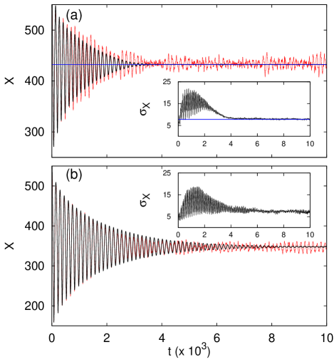
Figure 1: (color online) Irreversibility in the thermometer model: piston position in time for the non-interacting (a) and interacting (b) gas. Black and red curves denote ensemble averaged and single-realization trajectory, respectively. Blue horizontal lines denote the equilibrium values in the one-dimensional non-interacting case. Insets: standard deviation, $\sigma_{X}(t)$. Simulation parameters: $N=1024$, $m=1$, $M=50$, $F=150$, $T_{0}=10$, $X_{0}=600$. In the interacting case the pipe cross-section is $L=30$ and the interaction intensity $U_{0}=1$. Averages are over $2000$ (a) and $150$ (b) realizations.

Figure 2: (color online) Sensitive dependence on initial conditions in the interacting gas model. Typical evolution of the distance between two trajectories of the system starting from two close initial conditions $\bm{X}(0)$ and $\bm{X}^{\prime}(0)$, with $||\delta{\bm{X}}(0)||=\left(\sum_{i=0}^{2N}(X_{i}^{\prime}(0)-X_{i}(0))^{2}\right)^{1/2}=10^{-6}$. The distance $||\delta{\bm{X}}(t)||$ increases exponentially with time with rate given by the maximal Lyapunov exponent, $\lambda_{1}\approx 6$. All the parameters are the same of Fig.1.

We now discuss irreversibility by following the time evolution of the piston position in the interacting and non-interacting case. At time $t=0$, we fix the position of the piston $X(0)=X_{0}$, its velocity $V(0)=0$, and set the initial microscopic state as an equilibrium configuration of the gas in the volume imposed by the piston position at a given temperature $T_{0}$. In practice, we take the gas particles uniformly distributed in $[0:X_{0}]$ (in the two-dimensional case, in $[0:X_{0}]\times[0:L]$) with a Maxwell-Boltzmann distribution of velocities at temperature $T_{0}$.

We run molecular dynamics simulation by using event-driven schemes in the non-interacting gas and Verlet algorithm with time step $\Delta t=10^{-3}$ in the interacting one (see caption of Fig. 1 for specific parameters). As expected, numerical simulations show that when the initial state is sufficiently far from from equilibrium, meaning that $|X_{0}-X_{eq}|\gg\sigma_{X}^{eq}$, its evolution $X(t)$ exhibits an irreversible behavior.

Figure 1a reports a single trajectory, $X(t)$, and the behavior of the ensemble average, $\langle X(t)\rangle$, obtained by repeating the simulation from the same macroscopic initial condition (the same $X_{0}$ and $T_{0}$) but different microscopic initializations of the gas particles. We fixed $|X_{0}-X_{eq}|\approx 10\,\sigma_{X}^{eq}$. In analogy with the Ehrenfest model, we observe that the average trajectory is also typical: far from equilibrium, fluctuations are small compared to the ensemble average value. In other words, for almost every initial configuration of the system compatible with the macroscopic state, the time evolution of the piston position is practically identical to the average one. The standard deviation of the position, $\sigma_{X}(t)$, as shown in the inset of Fig. 1a, evolves from the initial value $0$ (by construction) and reaches the equilibrium value at long time, similarly to the Ehrenfest model but with a richer and more complex phenomenology. In particular, we notice the non-monotonic behavior of $\sigma_{X}(t)$ in the short-time oscillatory phase. Similar behaviors are not uncommon for systems starting from an unstable state [21]. However, and interestingly for our discussion, $\sigma_{X}(t)$ remains small with respect to the average value. We can thus observe macroscopic irreversibility in a single trajectory of macroscopic system initialized in a non-equilibrium initial state.

The interacting particle system (13) qualitatively displays the same behavior (Fig. 1b) supporting the statement that (microscopic) chaos does not add any new relevant feature to macroscopic irreversibility.

Figure 3: (color online) Evolution from close-to equilibrium initial conditions, (a) and (b), or for small systems (c). Piston position $X$ vs time for the non-interacting gas system: (a) with $N=1024$, $T_{0}=10$ and $X_{0}=X_{eq}+3\,\sigma_{X}^{eq}$; (b) the time reversed trajectory of (a), as marked by the arrows; (c) with $N=4$, $T_{0}=10$, $M=40$, $F=15$ and $X_{0}=1.4\cdot T_{eq}$. Horizontal (blue) lines denote the microcanonical ensemble average position of the piston $X_{eq}$. Other parameters are as in Fig. 1.

Figure 3a displays the typical evolution from a (close-to) equilibrium initial condition, i.e. $|X_{0}-X_{eq}|\approx\sigma_{X}^{eq}$, in the non-interacting gas system. As one can see, irreversibility does not show up: the time reversed trajectory is basically indistinguishable from the forward trajectory (compare Figs. 3a and b). Irreversibility cannot be observed also when the system is small, i.e. the number of degrees of freedom ($N$) is small. In the last case no notion of typicality can be defined: it is even meaningless to speak of far-from-equilibrium initial conditions, as fluctuations are of the same magnitude of mean values. Though the evolution is statistically stationary, we cannot define a (thermodynamic) equilibrium state when $N$ is small. Therefore, Fig. 3 demonstrates the importance of having a large number of degrees of freedom and of starting from a very non-typical initial conditions for observing macroscopic irreversibility.

Summarizing, when an experiment is conducted, in each single realization, the evolution of a macroscopic observable is close to the ensemble average and, in addition, it exhibits irreversibility, irrespectively of the presence of chaos in the system provided that the system is truly macroscopic ($N\gg 1$) and the initial condition is far (enough) from equilibrium. We remark that (microscopic) chaos is irrelevant also for dynamical transport properties close to equilibrium [22].

3.2 The adiabatic piston

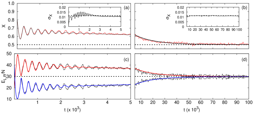
Figure 4: (color online) Irreversibility in the adiabatic piston: (a,b) piston position in a single realization (red) and ensemble average (black). Inset: evolution of the standard deviation $\sigma_{X}$. (c,d) Ensemble average of the left $E_{L}(t)/N$ (blue) and right $E_{R}(t)/N$ (red) kinetic energy per particle, and in a single realization (black). Horizontal (dashed) lines denote equilibrium values. The splitting in two panels (for short times (a,c) and longer times (b,d)) is just for an easier identification of the two regimes discussed in the text. The simulation parameters are $N=10^{3}$, $m=1$, $M=100$, $\mathcal{L}=2N$; the initial state is defined by $X_{0}=0.8$ with $T_{L}(0)=40$ and $T_{R}(0)=80$, averages are on $2000$ realizations.

We now consider the so-called adiabatic piston – a classical problem in non-equilibrium thermodynamics [23, 24, 20, 25] (see also Ref. [26] for a pedagogical introduction). In this interesting example the approach to equilibrium from a non-equilibrium state is characterized by a more complex phenomenology than that of the previous example.

In a nutshell the system is as follows. A thermo-mechanically isolated cylinder of length $\mathcal{L}$ is partitioned into two compartments by an adiabatic, freely-moving wall (the piston) of mass $M$. Each compartment contains a gas composed of $N$ non-interacting particles of mass $m$, elastically colliding with the walls. Thanks to the absence of direct interaction, we can restrict our analysis to one dimension, along the horizontal direction. The system is initialized with the piston kept fixed by a clamp at a given position, $X_{0}\mathcal{L}$; the non-interacting gases in the left/right (L/R) compartments are both in equilibrium, meaning that they are uniformly distributed in the compartments with volumes $V_{L}(0)=X_{0}\mathcal{L}$ and $V_{R}(0)=\mathcal{L}(1-X_{0})$, and velocities distributed with the Maxwell-Boltzmann distribution at different temperatures $T_{L,R}(0)$; the pressures are fixed by the non-interacting-gas state equation $P_{L,R}(0)V_{L,R}(0)=NT_{L,R}(0)$. Being the piston adiabatic, until the clamp is present, the two subsystems are in equilibrium even if $T_{L}(0)\neq T_{R}(0)$. At $t\!=\!0$, the clamp is removed and the piston is free to move without friction under collisions with gas particles. The non-trivial question is to predict the final position of the piston and values of thermodynamic quantities.

A careful treatment [27], within the framework of equilibrium thermodynamics, shows that the system should reach mechanical equilibrium $P_{L}=P_{R}$. However, the final position of the piston and gas temperatures remain undetermined. The prediction of the final equilibrium state needs to understand the non-equilibrium process, occurring after the clamp removal. Feynman [23] argued that the system first converges toward a state of mechanical equilibrium with $P_{R}\approx P_{L}$ (but for small fluctuations), consistently with the equilibrium thermodynamic prediction. Then, pressure fluctuations, which are asymmetric because of $T_{L}\neq T_{R}$, slowly drive the system toward thermal equilibrium $T_{R}=T_{L}$. The final position of the piston is $X_{eq}=1/2$ with standard deviation $\sigma_{X}^{eq}=1/(\sqrt{8N})$ [28]. The equilibrium temperature, $T^{eq}_{L}=T^{eq}_{R}=(T_{L}(0)+T_{R}(0))/2+O(1/N)$, can be directly derived from the conservation of energy fixed by the initial value $E=N((T_{L}(0)+T_{R}(0))/2$. Despite many attempts [29, 30, 20, 31] to derive Feynman predictions within a consistent analytic framework is a not yet solved problem even for non-interacting gases.

Here, our interest is to show that the scenario for macroscopic irreversibility so far discussed well applies also to this more complex irreversible process, characterized by the two regimes identified by Feynman.

In Figure 4, we show the irreversible macroscopic evolution of the system by monitoring the piston position and the kinetic energy per particle in each compartment $E_{L,R}(t)/N$ that, when the gases in each chamber are in equilibrium, are nothing but half the temperature values. Analogously to the previous section, we show both the evolution averaged over many realizations with the same initial macroscopic state and a single realization. Panels (a,c) refer to the first stage of the evolution ending with the equilibration of pressures; panels (b,d) pertain to the second stage in which, while $P_{L}\approx P_{R}$, asymmetric pressure fluctuations drive the system towards the final equilibrium state. The insets show the time evolution of the standard deviation of the piston position $\sigma_{X}(t)$ which behaves similarly to the thermometer model. As clear from the figure in both regimes any single trajectory closely traces the average one, a manifestation of typicality as previously discussed and a further demonstration of the validity of Boltzmann’s scenario for irreversibility, also in this non-trivial example.

4 Spreading of an “ink” drop

When an ink drop falls into the water, we observe its irreversible spreading and mixing with the fluid. A typical way to describe the phenomenon is in terms of the diffusion equation. The idea underlying such approach is to mimic the collisions of an ink molecule against water molecules by a stochastic force, renouncing to a deterministic description. Another possibility, within the deterministic framework, is to use molecular dynamics, but this can be very heavy from a computational point of view.

Here, we introduce an idealized simple model which can be used to study such a phenomenon from a conceptual point of view. We study a discrete-time high dimensional symplectic map (akin to a high dimensional Hamiltonian system) involving $2N$ degrees of freedom, and $2$ auxiliary variables. We consider a special case of the system proposed in Ref.  [32], in particular

$$\left\{\begin{array}[]{lll}y_{i}(t+1)&=&y_{i}(t)+\epsilon\cos[x_{i}(t)-\theta(t)]\\ x_{i}(t+1)&=&x_{i}(t)+y_{i}(t+1)\\ J(t+1)&=&J(t)-\epsilon\sum_{j=1}^{N}\cos[x_{j}(t)-\theta(t)],\\ \theta(t+1)&=&\theta(t)+J(t+1)\,.\end{array}\right.$$ (14)

Each pair $(x_{i},y_{i})$ identifies a “particle” ($i=1,\ldots,N$), and periodic boundary conditions on the two-dimensional torus $\mathbb{T}_{2}=[0,2\pi]\times[0,2\pi]$ are assumed. For $\epsilon=0$, the particles do not interact, while when $\epsilon>0$ (in our numerical examples we use $\epsilon=1$) particles interact (the “collisions” of water molecules) via a mean-field-like interaction, mediated by the variables $\theta$ and $J$. We emphasize that $\theta$ and $J$ do not have a precise physical meaning, they represent a simple mathematical expedient to introduce the interaction among particles in a symplectic manner. Moreover, the mean field character of the interaction is immaterial here and it simply allows fast numerical computation. In the presence of interactions the system exhibits complex evolutions, as realistic gases or liquids in molecular dynamics systems. System (14) can be shown to be time-reversible, see Ref. [33] for a detailed discussion on time reversal symmetries of discrete-time dynamical systems).

Figure 5: (color online) Irreversible spreading of an ink drop of $N_{I}=3.2\cdot 10^{3}$ particles on the Torus $\mathbb{T}_{2}$ at $t=0,4\cdot 10^{3},2.9\cdot 10^{4},2.33\cdot 10^{5}$ (in clockwise order from top left). The $N_{I}$ ink particles start uniformly distributed in $Q_{0}\equiv[0.3:1.3]\times[0.3:1.3]$, while the $N_{W}=10^{7}$ solvent ones have been thermalized in a previous time integration. The instantaneous occupation $n(t)$ is monitored in the (red) box $Q$ centered in $(\pi,\pi)$ with side $\pi/5$.

We used a system with interacting particles to avoid confusion between the genuine thermodynamic irreversibility and the mixing property, Eq. (3). As already stressed in Sec. 2.1, since our system is composed of $N$ interacting elements it should be clear that we are dealing with a single large system and not with a collection of different initial conditions as if the particles were non-interacting and evolving according to a generic mixing map of the torus. In this respect, we emphasize that the details of the interaction among the particles are not particularly important provided some form of interaction is present.

After several iterations, the system (14) reaches an “equilibrium” dynamical state characterized by a uniform distribution of particles on $\mathbb{T}_{2}$. To mimic the spreading of a cloud of “ink”, we split the $N$ particles into $N_{W}$ particles of solvent (water) and $N_{I}$ particles of solute (ink), with $N=N_{W}+N_{I}$ and $N_{I}\ll N_{W}$. Then, we prepare the initial condition of the system with the $N_{W}$ particles at equilibrium (e.g. after a long integration with $N_{W}$ particles only), and the solute particles uniformly distributed in a small region $Q_{0}$ of $\mathbb{T}_{2}$ (top left panel in Fig. 5). During the evolution, to measure the degree of mixing, we monitor the number of ink particles, $n(t)$, which at time $t$ reside in a given set $Q\subseteq\mathbb{T}_{2}$ (the red box $Q$ in Fig. 5). At equilibrium, when ink is well mixed, the $N_{I}$ particles will also distribute uniformly over $\mathbb{T}_{2}$, and thus $n(t)$ will fluctuate around $n_{eq}=N_{I}\mathcal{A}(Q)/\mathcal{A}(\mathbb{T}_{2})$, where $\mathcal{A}(Q)$ is the area of the subset $Q$.

It is instructive to compare (see Fig. 6) the behavior of $n(t)$ for a single trajectory with the average $\langle n(t)\rangle$, computed over an ensemble of many independent releases of the ink drop, with the water in different (microscopic) initial conditions arbitrarily chosen in the equilibrium state. Moreover, we study the difference between the case $N_{I}\sim O(1)$ (Fig. 6a) and $N_{I}\gg 1$ with $N_{I}\ll N_{W}$ (Fig. 6b). It is important to realize that while the latter case ($N_{I}\gg 1$) the ink drop can be considered a macroscopic object, in the former ($N_{I}\sim O(1)$) it cannot. In both cases, we observe that $\langle n(t)\rangle/n_{eq}$ increases monotonically with $t$, asymptotically approaching $1$. However, a dramatic difference emerges if we look at the single realization. For a (macroscopically well defined) drop with $N_{I}\gg 1$, the single trajectory closely follows the average one (Fig. 6b), and we can define an irreversible behavior for the individual drop. Conversely, when $N_{I}\sim O(1)$, the single trajectory is indistinguishable from its time reverse one (Fig. 6a) and strongly differs from the average one. The latter apparently shows a form of irreversibility, but it is thus a mere artifact of the average over the initial distribution and the special initial condition. We stress that, the lack of irreversibility in this case is due to the fact that, being $N_{I}$ small, $n(t)$ cannot be considered a macroscopic observable even if the system water plus drop is large ($N\gg 1$), as $n(t)$ depends only on the few “molecules” of ink.

Figure 6: Instantaneous occupation $n(t)/n_{eq}$ of the set $Q$ (blue, fluctuating curve) and its average $\langle n(t)\rangle/n_{eq}$ (black, smooth curve) over 500 independent initial conditions starting from $Q_{0}$: (a) $n_{eq}=0.3$ (drop with very few particles, $N_{I}=8$ and $N_{W}=2500$) and (b) $n_{eq}=10^{3}$ (drop with many particles $N_{I}=2.5\times 10^{4}$ and $N_{W}=10^{6}$).

5 Final Remarks

In this work, with the help of numerical simulations of simple, yet non-trivial, Hamiltonian models, we revisited some of the basic aspects of Boltzmann’s interpretation of irreversibility. It is worth concluding by listing some of the key elements underlined by our simple investigation.

1. Irreversibility is observed and must be defined in a single macroscopic body. This implies that averaging over all the possible initial conditions is unnecessary both at a practical and conceptual level, as perfectly obvious to experimentalists.

2. Crucial to observe irreversibility is the choice of the initial condition, which has to be very “unlikely”, that is sufficiently far-from equilibrium. Indeed, even in a large-$N$ system, irreversibility does not show up in a trajectory starting from initial conditions chosen close-to-equilibrium (see Fig. 3a and b).

3. Irreversibility is a property of macroscopic bodies, i.e. of system with a large number of components $N\gg 1$. Indeed, the large $N$ condition of a system grants that it develops a “typical” behavior, meaning that the features of a single system are close to their averages.

4. The presence, or absence, of chaos is not relevant. Chaos plays a role in mixing, which is surely a form of “irreversibility”, but which has nothing to do with the second law.

All the irreversible behaviors in the approach to equilibrium that we observed in the examined examples clearly confirm the above conceptual framework whenever the system is composed of a large number of particles and the observables are macroscopic, i.e. depend upon a large number of degrees of freedom. Conversely, when either the number of particles is small or the observed quantity depends on few degrees of freedom, we are unable to identify a clear trend towards equilibrium and we cannot determine the time arrow.

References

- [1] J. L. Lebowitz, Boltzmann’s entropy and time’s arrow, Physics today 46 (1993) 32–32.
- [2] C. Cercignani, Ludwig Boltzmann: the man who trusted atoms, Oxford University Press, 2006.
- [3] S. Chibbaro, L. Rondoni, A. Vulpiani, Reductionism, Emergence and Levels of Reality, Springer, 2014.
- [4] O. E. Lanford III, Time evolution of large classical systems, in: Dynamical systems, theory and applications, Springer, 1975, pp. 1–111.
- [5] H. Barnum, C. M. Caves, C. Fuchs, R. Schack, D. J. Driebe, W. G. Hoover, H. Posch, B. L. Holian, R. Peierls, J. L. Lebowitz, Is Boltzmann entropy time’s arrow’s archer?, Physics Today 47 (11) (2008) 11–117.
- [6] S. Goldstein, Typicality and notions of probability in physics, in: Y. Ben-Menahem, M. Hemmo (Eds.), Probability in physics, Springer, 2012, pp. 59–71.
- [7] N. Zanghì, I fondamenti concettuali dell’approccio statistico in fisica, in: V. Allori, M. Dorato, F. Laudisa, N. Zanghì (Eds.), La natura delle cose: Introduzione ai fondamenti e alla filosofia della fisica, Carocci, 2005, pp. 202–247.
- [8] I. Prigogine, I. Stengers, Order out of chaos, Bantam Books, 1994.
- [9] J. Bricmont, Science of chaos or chaos in science, Pysicalia Mag. 17 (1995) 159.
- [10] S. Goldstein, Boltzmann’s approach to statistical mechanics, in: Chance in physics, Springer, 2001, pp. 39–54.
- [11] K. Huang, Statistical mechanics, Wiley, New York, 1988.
- [12] M. Kac, Probability and related topics in physical sciences, Vol. 1, American Mathematical Soc., 1957.
- [13] R. H. Swendsen, Explaining irreversibility, American Journal of Physics 76 (7) (2008) 643–648.
- [14] P. Ehrenfest, T. Ehrenfest, The conceptual foundation of the statistical approach in mechanics, Cornell University Press, New York, 1956, (trasl. from 1911 German version.
- [15] P.-M. Binder, J. Pedraza, S. Garzón, An invertibility paradox, American Journal of Physics 67 (12) (1999) 1091–1093.
- [16] P. Castiglione, M. Falcioni, A. Lesne, A. Vulpiani, Chaos and coarse graining in statistical mechanics, Cambridge University Press Cambridge, 2008.
- [17] H. Risken, Fokker-Planck Equation, Springer, 1984.
- [18] M. Falcioni, D. Villamaina, A. Vulpiani, A. Puglisi, A. Sarracino, Estimate of temperature and its uncertainty in small systems, American Journal of Physics 79 (7) (2011) 777–785.
- [19] L. Cerino, G. Gradenigo, A. Sarracino, D. Villamaina, A. Vulpiani, Fluctuations in partitioning systems with few degrees of freedom, Physical Review E 89 (4) (2014) 042105.
- [20] N. Chernov, J. Lebowitz, Dynamics of a massive piston in an ideal gas: Oscillatory motion and approach to equilibrium, Journal of Statistical Physics 109 (3-4) (2002) 507–527.
- [21] F. De Pasquale, P. Tartaglia, P. Tombesi, Stochastic dynamic approach to the decay of an unstable state, Zeitschrift für Physik B Condensed Matter 43 (4) (1981) 353–360.
- [22] F. Cecconi, M. Cencini, A. Vulpiani, Transport properties of chaotic and non-chaotic many particle systems, Journal of Statistical Mechanics: Theory and Experiment 2007 (12) (2007) P12001.
- [23] R. P. Feynman, R. Leighton, M. Sands, Lectures in Physics I, Addison-Wisley, New York, 1965.
- [24] E. H. Lieb, Some problems in statistical mechanics that i would like to see solved, Physica A: Statistical Mechanics and its Applications 263 (1) (1999) 491–499.
- [25] C. Gruber, A. Lesne, The adiabatic piston, in: J. P. Francoise, G. Naber, T. Tsun (Eds.), Modern Encyclopedia of Mathematical Physics, Vol. 1, Elsevier, 2006.
- [26] B. Crosignani, P. Di Porto, M. Segev, Approach to thermal equilibrium in a system with adiabatic constraints, American Journal of Physics 64 (5) (1996) 610–613.
- [27] A. Curzon, A thermodynamic consideration of mechanical equilibrium in the presence of thermally insulating barriers, American Journal of Physics 37 (4) (1969) 404–406.
- [28] E. DelRe, B. Crosignani, P. Di Porto, S. Di Sabatino, Built-in reduction of statistical fluctuations of partitioning objects, Physical Review E 84 (2) (2011) 021112.
- [29] C. Gruber, G. P. Morriss, A Boltzmann equation approach to the dynamics of the simple piston, Journal of statistical physics 113 (1-2) (2003) 297–333.
- [30] M. M. Mansour, C. Van Den Broeck, E. Kestemont, Hydrodynamic relaxation of the adiabatic piston, EPL (Europhysics Letters) 69 (4) (2005) 510.
- [31] M. Cencini, L. Palatella, S. Pigolotti, A. Vulpiani, Macroscopic equations for the adiabatic piston, Physical Review E 76 (5) (2007) 051103.
- [32] G. Boffetta, D. del Castillo-Negrete, C. López, G. Pucacco, A. Vulpiani, Diffusive transport and self-consistent dynamics in coupled maps, Physical Review E 67 (2) (2003) 026224.
- [33] J. Roberts, G. Quispel, Chaos and time-reversal symmetry. order and chaos in reversible dynamical systems, Phys. Rep. 216 63–177.