Time Synchronization of Turbo-Coded Square- QAM-Modulated Transmissions: Code-Aided ML Estimator and Closed-Form Cramér-Rao Lower Bounds

Abstract

This paper introduces a new maximum likelihood (ML) solution for the code-aided (CA) timing recovery problem in square-QAM transmissions and derives, for the very first time, its CA Cram r-Rao lower bounds (CRLBs) in closed-form expressions. By exploiting the full symmetry of square-QAM constellations and further scrutinizing the Gray-coding mechanism, we express the likelihood function (LF) of the system explicitly in terms of the code bits’ a priori log-likelihood ratios (LLRs). The timing recovery task is then embedded in the turbo iteration loop wherein increasingly accurate estimates for such LLRs are computed from the output of the soft-input soft-output (SISO) decoders and exploited at a per-turbo-iteration basis in order to refine the ML time delay estimate. The latter is then used to better re-synchronize the system, through feedback to the matched filter (MF), so as to obtain more reliable symbol-rate samples for the next turbo iteration. In order to properly benchmark the new CA ML estimator, we also derive for the very first time the closed-form expressions for the exact CRLBs of the underlying turbo synchronization problem. Computer simulations will show that the new closed-form CRLBs coincide exactly with their empirical counterparts evaluated previously using exhaustive Monte-Carlo simulations. They will also show unambiguously the remarkable performance improvements of CA estimation against the traditional non-data-aided (NDA) scheme; thereby highlighting the potential performance gains in time synchronization that can be achieved owing to the decoder assistance. Over a wide range of practical SNRs, CA estimation becomes even equivalent to the completely data-aided (DA) scheme in which all the transmitted symbols are perfectly known to the receiver. Moreover, the new CA ML estimator almost reaches the underlying CA CRLBs, even for small SNRs, thereby confirming its statistical efficiency in practice. It also enjoys significant improvements in computational complexity as compared to the most powerful existing ML solution, namely the combined sum-product and expectation-maximization (SP-EM) algorithm.

I Introduction

In order to provide high quality of service while satisfying the ever-increasing demand in high data rates, the use of powerful error-correcting codes in conjunction with high-spectral-efficiency modulations is advocated. Indeed, turbo codes along with high-order quadrature amplitude modulations (QAMs) are two key features of current and future wireless communication standards such as 4G long-term evolution (LTE), LTE-advanced (LTE-A) and beyond (LTE-B) [References, References]. As a crucial task in any digital receiver [References], accurate time synchronization remains a challenging problem especially for turbo-coded systems since they are intended to operate at very low signal-to-noise ratios (SNRs). In fact, the widespread adoption of turbo codes is in part fueled by their ability to operate in the near-Shannon limit even under such adverse SNR conditions [References]. Yet, the salutary performance of these powerful error-correcting codes is prone to severe degradations if the system is not accurately synchronized in time, phase or frequency. The goal of time synchronization, in particular, consists in estimating and compensating for the unknown time delay introduced by the channel so as to provide the decision device with symbol-rate samples of lowest possible inter-symbol interference (ISI) corruption [References].
The problem of timing recovery for linearly-modulated transmissions has been heavily investigated over the last few decades. A plethora of time delay estimators (TDEs) have been introduced in the open literature and the vast majority of existing TDEs are intended to operate with complete unawareness of the code structure (see [References-References] and references therein). In other words, the TD estimate is acquired just after oversampling the continuous-time signal and then provided to a discrete-time MF in order to output the symbol-rate samples. The latter are then used by the turbo decoder, once for all, to decode the data bits. Therefore, the fact that a large portion of the data bits is to become almost perfectly known (i.e., correctly decoded) is systematically ignored by those estimators. The latter are referred to as non-code-aided (NCA) or simply NDA TDEs since no a priori knowledge about the transmitted symbols is used during the estimation process and, as such, they suffer from severe performance degradations under harsh SNR conditions. Being more accurate and usually less computationally expensive, DA methods require, however, the regular transmission of a completely known (i.e., pilot) sequence thereby limiting the whole throughput of the system.
It sounds reasonable then to conceive a third alternative as a middle ground between these two extreme NDA and DA estimation schemes. Indeed, rather than relying on perfectly known or completely unknown symbols, CA estimation takes advantage of the soft information delivered by the decoder at each turbo iteration. In plain English, the decoder assistance is called upon in an attempt to enhance the timing recovery capabilities yet with no impact on the spectral efficiency of the system. In fact, from one turbo iteration to another, more refined soft information about the conveyed bits are delivered by the two soft-input soft-output (SISO) decoders. These are $i)$ the a posteriori LLRs of the code bits and $ii)$ their extrinsic information. According to the turbo principle, the latter are iteratively exchanged between the two SISO decoders until achieving a steady state whose a posteriori LLRs are used as decision metrics for data detection. In a nutshell, CA estimation consists simply in leveraging those soft outputs, by embedding the timing recovery task into the decoding process, in an attempt to enhance the estimation performance and vice versa. In the context of timing, phase, and frequency recovery, such CA estimation scheme is usually referred to as turbo synchronization [References]. A number of CA timing recovery algorithms have been proposed over the last decade [References-References] and, to the best of the authors’ knowledge, only two approaches are derived from ML theory. The first one [References] is based on the well-known expectation maximization (EM) algorithm whereas the second [References] is a combined sum-product (SP) and EM algorithm approach (i.e., an improvement of [References]). The SP-EM-based ML estimator offers indeed significant performance improvements over the original EM-based estimator but at the cost of increased computational complexity. In the SP-EM-based ML approach, an EM iteration loop is required in each turbo iteration wherein the algorithm stwitches between the so-called expcetation step (E-STEP) and maximization step (M-STEP). Roughly speaking, in each turbo iteration, the algorithm performs the following main four steps for each EM iteration:

• Obtain new symbol-rate samples (via MF) using the TD estimate of the previous EM iteration;

• Update the symbols’ a posteriori probabilities (APoPs) using those new symbol-rate samples;

• Marginalize empirically the conditional (on the transmitted symbols) likelihood function with respect to those APoPs (E-STEP) ;

• Maximize the marginalized LF with respect to the working TD variable (M-STEP).

At the convergence of the EM algorithm, the obtained TD estimate is used to acquire new ISI-reduced (symbol-rate) samples which will serve as input for the next turbo iteration where all the aforementioned EM-related steps are repeated.
In this paper, we re-consider the problem of CA time synchronization from both the “performance bounds” and “algorithmic” point of views. By exploiting the full symmetry of square-QAM constellations and further scrutinizing the Gray coding mechanism, we are able to derive a closed-form and very simple expression for the system’s LF. Typically, marginalization of the conditional LF with respect to transmitted symbols is carried-out analytically and the a priori LLRs of the elementary code bits are explicitly incorporated in the LF expression. We propose thereof a more systematic framework to their direct integration in the CA estimation process, thereby eliminating completely the need for the EM iteration loop under each turbo iteration. In other words, the new LF needs to be maximized only once per-turbo iteration (contrarily to SP-EM) after being updated by the associated a priori LLRs which are computed from the output of the SISO decoders. Consequently, the proposed CA timing recovery algorithm offers significant improvements in computational complexity as compared to the existing SP-EM. As a matter of fact, the new algorithm is 35 and 70 times less computationally complex than SP-EM for 64 and 256 QAMs, respectively. It also enjoys an advantage in terms of estimation accuracy for low SNR levels and higher-order modulations.
From the “performance bounds” point of view, we also tackle the analytical derivation of the stochastic CRLBs for the underlying CA estimation problem. Actually, unlike many other loose bounds, the stochastic CRLB is a fundamental lower bound that reflects the actual achievable performance in practice [References]. Yet, even under uncoded transmissions, the complex structure of the LF makes it extremely hard, if not impossible, to derive analytical expressions for this practical bound, especially with high-order modulations. Therefore, in the specific context of timing recovery, the stochastic CRLBs were previously evaluated using exhaustive Monte-Carlo simulations (i.e., empirically) in [References] and [References] for both NCA and CA estimations, respectively. Just recently though were their analytical expressions established [References] but only in the NCA (i.e., NDA) case.
In this paper, we succeed in factorizing the LF of the coded system as the product of two analogous terms involving two random variables that are almost identically distributed, i.e., their probability density functions (pdfs) have the same expression but parametrized differently. We then capitalize on this interesting property to derive, for the very first time, the closed-form expressions for the TD CA CRLBs from arbitrary turbo-coded square-QAM-modulated transmissions. The new closed-form expressions corroborate the previous attempts reported in [References] to evaluate the TD CA CRLBs empirically and offer a way to their immediate evaluation in practice. Moreover, as will be shown later, the previously published closed-form NDA CRLBs [References] boil down to a very special case of the new closed-form CA CRLBs by simply setting all the code bits’ a priori LLRs to zero.
The rest of this paper is structured as follows. In section II, we present the system model. In section III, we derive the expression of the log-likelihood function (LLF) and express it explicitly as function of the coded bits’ a priori LLRs. in Section IV, we establish the new closed-form expressions for the TD CA CRLBs. In Section V, we introduce the new CA ML time delay estimator. In Section VI, we discuss the simulation results of the proposed CA ML estimator and closed-form CRLBs. Finally, we draw out some concluding remarks in section VII.
We also mention beforehand that some of the common notations will be used in this paper. Vectors and matrices are represented in lower- and upper-case bold fonts, respectively. $\mathbf{I}_{N}$ and $\mathbf{0}_{N}$ denote, respectively, the $N\times N$ identity matrix and the $N-$dimensional all-zero vector. The shorthand notation $\mathbf{x}\sim\mathcal{N}(\mathbf{m},\mathbf{R})$ means that the vector $\mathbf{x}$ follows a normal (i.e., Gaussian) distribution with mean $\mathbf{m}$ and auto-covariance matrix $\mathbf{R}$. Moreover, $\{.\}^{T}$ and $\{.\}^{H}$ denote the transpose and the Hermitian (transpose conjugate) operators, respectively. The operators $\Re\{.\}$ and $\Im\{.\}$ return, respectively, the real and imaginary parts of any complex number. The operators $\{.\}^{*}$ and $|.|$ return its conjugate and its amplitude, respectively, and $j$ is the pure complex number that verifies $j^{2}=-1$. The Kronecker and Dirac delta functions are denoted, respectively, as $\delta_{m,n}$ and $\delta(t)$. We will also denote the probability mass function (PMF) for discrete random variables (RVs) by $P[.]$ and the pdf for continuous RVs by $p[.]$ The statistical expectation is denoted as $\mathbb{E}\{.\}$ and the notation $\triangleq$ is used for definitions.

II System Model

Consider a turbo-coded system where a binary sequence of information bits is fed into a turbo encoder consisting of two identical recursive and systematic convolutional codes (RSCs) which are concatenated in parallel via an inner interleaver $\Pi_{1}$. The resulting code bits are fed into a puncturer which selects an appropriate combination of the parity bits, from both encoders, in order to achieve a desired code rate $R$. The entire code bit sequence is then scrambled with an outer interleaver, $\Pi_{2}$, and divided into $K$ subgroups of $2p$ bits each for some integer $p\geq 1$. The $k^{th}$ subgroup of code bits, $b_{1}^{k}b_{2}^{k}\cdots b_{l}^{k}\cdots b_{2p}^{k}$, is conveyed by a symbol $a(k)$ that is selected from a fixed alphabet, $\mathcal{C}_{p}=\{c_{0},c_{1},\cdots,c_{M-1}\}$, of a $M-$ary (with $M=2^{2p}$) QAM constellation (i.e., square-QAM). In fact, each point, $c_{m}\in\mathcal{C}_{p}$, is mapped onto a unique sequence of $\log_{2}(M)=2p$ bits denoted here as $\bar{b}_{1}^{m}\bar{b}_{2}^{m}\cdots\bar{b}_{l}^{m}\cdots\bar{b}_{2p}^{m}$, according to the Gray coding mechanism, and the point $c_{m}$ is selected to convey the $k^{th}$ code bits subgroup [i.e., $a(k)=c_{m}$] if and only if $b_{l}^{k}=\bar{b}_{l}^{m}$ for $l=1,2,\cdots,2p$. We also define the a priori LLR of the $l^{th}$ code bit, $b^{k}_{l}$, conveyed by $a(k)$ as follows:

$$L_{l}(k)~{}\triangleq~{}\ln\left(\frac{P[b^{k}_{l}=1]}{{P[b^{k}_{l}=0]}}\right).$$ (1)

Using (1) and the fact that $P[b_{l}^{k}=0]+P[b_{l}^{k}=1]=1$, it can be easily shown that:

$$P[b_{l}^{k}=1]=\displaystyle\frac{e^{L_{l}(k)}}{1+e^{L_{l}(k)}}~{}~{}~{}~{}\textrm{and}~{}~{}~{}~{}P[b_{l}^{k}=0]=\displaystyle\frac{1}{1+e^{L_{l}(k)}}.$$ (2)

For mathematical convenience, the two identities in (2) can be merged together to yield the following common generic expression:

$$P[b_{l}^{k}=\bar{b}_{l}^{m}]\!=\!\frac{1}{2\cosh\big{(}L_{l}(k)/2\big{)}}{e^{(\bar{b}_{l}^{m}-1)\frac{L_{l}(k)}{2}}},$$ (3)

in which $\bar{b}_{l}^{m}$ is either $0$ or $1$ depending on which of the symbols $c_{m}$ is transmitted, at time instant $k$, and of course on the Gray mapping associated to the constellation. The obtained information-bearing symbols, $\{a(k)\}_{k=1}^{K}$, are then pulse-shaped and the resulting continuous-time signal:

$$x(t)=\sum_{k=1}^{K}a(k)~{}\!h(t-kT),$$ (4)

is transmitted over the communication channel with $T$ being the symbol duration and $h(t)$ a unit-energy square-root shaping pulse. Being completely unknown to the receiver a priori, the transmitted symbols $\{a(k)\}_{k}$ are drawn from a given $M$-ary Gray-coded (GC) square-QAM constellation whose alphabet is denoted as $\mathcal{C}_{p}=\{c_{0},c_{1},\cdots,c_{M-1}\}$. Here, by square QAM we mean $M=2^{2p}$ for some integer $p\geq 1$ (i.e., QPSK, $16-$QAM, $64-$QAM, etc…). The Nyquist pulse $g(t)$ obtained from $h(t)$ is defined as:

$$g(t)=\int_{-\infty}^{+\infty}h(x)h(t+x)dx,$$ (5)

and satisfies the first Nyquist criterion [References]:

$$g(nT)=0,~{}\textrm{for any integer}~{}n\neq 0.$$ (6)

At the receiver side, assuming perfect frequency and phase synchronizations, the (delayed) continuous-time received signal before matched filtering is expressed as:

$$y(t)=\sqrt{E_{s}}~{}x(t-\tau)~{}+~{}w(t),$$ (7)

where $E_{s}$ is the transmit signal energy and $\tau$ is the unknown time delay parameter to be estimated. Moreover, $w(t)$ is a proper complex additive white Gaussian noise (AWGN) with independent real and imaginary parts, each of variance $\sigma^{2}$ (i.e., with overall noise power $N_{0}=2\sigma^{2}$). The SNR of the channel is also denoted as:

$$\rho~{}\triangleq~{}\frac{E_{s}}{N_{0}}~{}=~{}\frac{E_{s}}{2\sigma^{2}}.$$ (8)

An integral step in the derivation of stochastic ML estimators and CRLBs consists in finding the LLF of the system. This requires marliginalizing the conditional (on the unknown symbols) LF over the constellation alphabet. In completely NDA estimation (or before data detection), no a priori information is available about the transmitted symbols. Therefore, the latter are usually assumed to be equally likely, i.e., with equal a priori probabilities (APPs). That is to say $\forall~{}\!c_{m}\in\mathcal{C}_{p}$:

$$P[a(k)=c_{m}]=\frac{1}{M}~{}~{}~{}~{}~{}~{}\textrm{for}~{}~{}k=1,2,\cdots,K.$$ (9)

In CA estimation, however, the actual APPs of the transmitted symbols must be used in order to enhance the estimation performance as done in the next section. By doing so, we will ultimately express the LLF explicitly as function of the a priori LLRs of the individual coded bits. As will be explained later in Section IV-E, accurate estimates for the underlying LLRs can be obtained in practice from the soft outputs of the two SISO decoders at the convergence of the BCJR algorithm [32].

III Derivation of the LLF

As widely known, the set of finite-energy signals usually denoted as:

$$\mathcal{L}^{2}_{\mathbb{R}}=\left\{s(t)~{}\textrm{such that}~{}\int_{\mathbb{R}}|s(t)|^{2}dt<+\infty\right\},$$

form an infinite-dimension Hilbert subspace [References] that can be endowed with an orthonormal basis $\{\varphi_{n}(t)\}_{n}$ and an inner product as follows:

$$\langle s_{1}(t),s_{2}(t)\rangle=\int_{\mathbb{R}}s_{1}(t)s_{2}(t)^{*}dt,~{}~{}\forall~{}s_{1}(t),s_{2}(t)\in\mathcal{L}^{2}_{\mathbb{R}}.$$ (10)

Therefore, an exact discrete representation for any continuous-time signal $s(t)\in\mathcal{L}^{2}_{\mathbb{R}}$ requires an infinite-dimensional vector, ${\bm{s}}$, that contains its expansion coefficients, $\big{\{}s_{n}=\langle s(t),\varphi_{n}(t)\rangle\big{\}}_{n}$, in the basis $\{\varphi_{n}(t)\}_{n}$. To sidestep this problem, we first consider the $N$-dimensional truncated representation vectors:

$$\bm{y}_{N} \!\!\!\!=\!\!\!\! \left[y_{1},y_{2},\ldots,y_{N}\right]^{T}\!\!,$$ (11)

$$\bm{w}_{N} \!\!\!\!=\!\!\!\! \left[w_{1},w_{2},\ldots,w_{N}\right]^{T}\!\!,$$ (12)

$$\bm{x}_{N}(\tau) \!\!\!\!=\!\!\!\! \left[x_{1}(\tau),x_{2}(\tau),\ldots,x_{N}(\tau)\right]^{T}\!\!.$$ (13)

that contain the orthogonal projection coefficients of $y(t)$, $w(t)$, and $x(t-\tau)$, respectively, over the first $N$ basis functions $\{\varphi_{n}(t)\}_{n=1}^{N}$ (for any $N\geq 1$), i.e.:

$$y_{n} \!\!\!\!=\!\!\!\! \big{\langle}y(t),\varphi_{n}(t)\big{\rangle}=\int_{\mathbb{R}}y(t)\varphi_{n}(t)^{*}dt,$$ (14)

$$w_{n} \!\!\!\!=\!\!\!\! \big{\langle}w(t),\varphi_{n}(t)\big{\rangle}=\int_{\mathbb{R}}w(t)\varphi_{n}(t)^{*}dt,$$ (15)

$$x_{n}(\tau) \!\!\!\!=\!\!\!\! \big{\langle}x(t-\tau),\varphi_{n}(t)\big{\rangle}=\int_{\mathbb{R}}x(t-\tau)\varphi_{n}(t)^{*}dt,$$ (16)

Using (7) and (14) to (16), it follows that:

$$\bm{y}_{N}=\sqrt{E_{s}}~{}\!\bm{x}_{N}(\tau)+\bm{w}_{N}.$$ (17)

Due to the orthogonality of the basis functions, it can be shown that the noise projection coefficients, $\{w_{n}\}_{n=1}^{N}$, explicitly given by (15) are uncorrelated, i.e, $\mathbb{E}\big{\{}w_{n}w_{m}^{*}\big{\}}=2\sigma^{2}\delta_{n,m}$. Hence, they are independent since they are also Gaussian-distributed leading to $\bm{w}_{N}\sim\mathcal{N}(\mathbf{0}_{N},2\sigma^{2}\mathbf{I}_{N})$. Therefore, the pdf of the vector ${\bm{y}}_{N}$ in (17) conditioned on the sequence of transmitted symbols, $\bm{a}=[a(1),a(2),\ldots,a(K)]^{T}$, and parametrized by $\tau$ is given by:

$$\!\!\!\!\!\!\!\!p({\bm{y}}_{N}|\bm{a};\tau) = \prod\displaylimits_{n=1}^{N}{\frac{1}{2\pi\sigma^{2}}}\exp\!\left\{\!-{\frac{1}{2\sigma^{2}}}\big{|}y_{n}\!-\!{{\sqrt{E_{s}}}}x_{n}(\tau)\big{|}^{2}\right\}.$$ (18)

Note here that, although we do not show it explicitly, the transmitted symbols are indeed involved in (18) via the coefficients $\{x_{n}(\tau)\}_{n}$. After dropping the constant terms that do not depend explicitly on $\tau$ in (18), we obtain the simplified truncated LF:

$$\!\!\!\!\!\!\!\!\!\!\!\!\Lambda({\bm{y}}_{N}|\bm{a};\tau) = \exp\!\left\{\!{\frac{\sqrt{E_{s}}}{\sigma^{2}}}\sum\displaylimits_{n=1}^{N}\!\Re\left\{y_{n}x_{n}(\tau)^{*}\right\}-{\frac{E_{s}}{2\sigma^{2}}}\!\sum_{n=1}^{N}\!\big{|}x_{n}(\tau)\big{|}^{2}\!\right\}.$$ (19)

The conditional LF which incorporates all the information contained in the non-truncated vector ${\bm{y}}$ [or equivalently the received continuous-time signal $y(t)$], is obtained by making $N$ tend to infinity in (19). By doing so and using the Plancherel equality, we obtain the following conditional LF:

$$\!\!\!\!\!\!\!\!\!\!\Lambda(\bm{y}|\bm{a};\tau) = \textstyle\exp\!\left\{\!\frac{\sqrt{E_{s}}}{\sigma^{2}}\!{\int_{\mathbb{R}}}\!\Re\big{\{}y(t)x(t\!-\!\tau)^{*}\big{\}}dt-\textstyle\frac{E_{s}}{2\sigma^{2}}{\int_{\mathbb{R}}}|x(t\!-\!\tau)|^{2}dt\!\right\}.$$ (20)

Now, replacing the transmitted signal $x(t)$ by its expression given in (4), and exploiting the fact that the shaping pulse, $g(t)$, in (5) verifies the first-order Nyquist criterion (6), it can be shown that:

$$\Lambda(\bm{y}|\bm{a};\tau) \!\!\!\!=\!\!\!\! \prod_{k=1}^{K}\Omega_{\tau}\big{(}a(k),y(t)\big{)},$$ (21)

where

$$\!\!\!\!\!\!\!\!\!\!\!\!\Omega_{\tau}\big{(}a(k),y(t)\big{)} \triangleq \exp\!\left\{\!{\frac{\sqrt{E_{s}}}{\sigma^{2}}}\!\!\!\int_{\mathbb{R}}\!\!\Re\big{\{}y(t)a(k)^{*}\!\big{\}}h(t\!-\!kT\!-\!\tau)dt\!-\!{\frac{E_{s}}{2\sigma^{2}}}\big{|}a(k)\big{|}^{2}\right\}.$$ (22)

The unconditional LF, $\Lambda(\bm{y};\tau)$, is obtained by averaging (21) over all possible transmitted symbol sequences of size $K$, i.e., $\Lambda(\bm{y};\tau)=\mathbb{E}_{\bm{a}}\{\Lambda(\bm{y}|\bm{a};\tau)\}$ leading to:

$$\Lambda(\bm{y};\tau) \!\!\!\!=\!\!\!\! \sum_{\bm{c}_{i}\in\mathcal{C}_{p}^{K}}P[\bm{a}=\bm{c}_{i}]\Lambda(\bm{y}|\bm{a}=\bm{c}_{i};\tau).$$ (23)

Under coded digital transmissions, a simplifying assumption is usually used in estimation practices, whether CA or NCA, in order to allow for tractable mathematical derivations of CRLBs and ML estimators of any parameter. This assumption postulates that the transmitted symbols are independent (cf. [References-References] and references therein) in spite of the statistical dependence between the coded bits that is introduced by channel coding. In fact, before even initiating the decoding process itself, the system needs to be fully synchronized by estimating the time delay, as well as, the phase and frequency offsets. Moreover, the decoder itself needs some estimates for other key channel parameters, e.g., the channel coefficient, noise variance, SNR, etc. All those estimates are obtained by applying traditional NDA estimators directly on the symbol-rate samples that are delivered by the matched filter before starting data decoding. As a matter of fact, in digital transmissions, all state-of-the-art NDA estimators (for any parameter, whether maximum likelihood or moment-based) are indeed based on the assumption of independent symbols although the latter are actually dependent due to channel coding.
We emphasize, however, that exploitation of this assumption does not imply denying to exploit the dependence of the coded bits during the decoding process itself. Indeed, such dependence is exploited by the SISO decoders in order to output the estimates for the coded bits’ a posteriori LLRs. The latter are then used to decode the bits and also to compute their a priori LLRs (as explained later in Section IV-E) which are in turn used to evaluate the CA CRLBs and to find the CA TD ML estimate. Yet, even by assuming independent symbols (both in this paper and all existing works), it turns out that no much information is lost from the estimation point of view. In fact, the resulting CA estimation schemes achieve the ideal data-aided one (where all the symbols are perfectly known) over a wide range of practical SNRs where the completely NDA schemes do not (cf. Figs. 4 and 5 in this paper and the reported simulation results in other researchers’ works). Using the assumption of independent symbols it follows that:

$$P\big{[}\bm{a}=\bm{c}_{i}\big{]}=\prod_{k=1}^{K}P\big{[}a(k)=\bm{c}_{i}(k)\big{]}.$$ (24)

Plugging (21) and (24) in (23), it can be shown that:

$$\!\!\!\!\!\!\!\!\Lambda(\bm{y};\tau) \!\!\!\!=\!\!\!\! \sum_{\bm{c}_{i}\in\mathcal{C}_{p}^{K}}\prod_{k=1}^{K}P\big{[}a(k)=\bm{c}_{i}(k)\big{]}\Omega_{\tau}\big{(}\bm{c}_{i}(k),y(t)\big{)}$$ (25)

$$\!\!\!\!=\!\!\!\! \prod_{k=1}^{K}\sum_{c_{m}\in\mathcal{C}_{p}}P\big{[}a(k)=c_{m}\big{]}\Omega_{\tau}\big{(}c_{m},y(t)\big{)}.$$

Therefore, the unconditional log-likelihood function (LLF) defined as $\mathcal{L}(\bm{y};\tau)\triangleq\ln\big{(}\Lambda(\bm{y};\tau)\big{)}$, is given by:

$$\mathcal{L}(\bm{y};\tau) \!\!\!\!=\!\!\!\! \sum_{k=1}^{K}\ln\Big{(}\bar{\Omega}_{k}\big{(}\tau,y(t)\big{)}\Big{)},$$ (26)

in which $\bar{\Omega}_{k}\big{(}\tau,y(t)\big{)}$ is simply the average of $\Omega_{\tau}\big{(}a(k),y(t)\big{)}$ over the constellation alphabet, i.e.:

$$\bar{\Omega}_{k}\big{(}\tau,y(t)\big{)} \!\!\!\!\triangleq\!\!\!\! \sum_{c_{m}\in\mathcal{C}_{p}}P\big{[}a(k)=c_{m}\big{]}\Omega_{\tau}\big{(}c_{m},y(t)\big{)}.$$ (27)

For ease of notations, we will hereafter no longer show the dependence of $\bar{\Omega}_{k}\big{(}\tau,y(t)\big{)}$ on the received signal, $y(t)$, and denote it simply as $\bar{\Omega}_{k}(\tau)$. Next, we will further manipulate this term and ultimately factorize it into two analogous terms which involve two independent and almost identically distributed RVs. In fact, by further denoting the top-right quadrant of the constellation as $\widetilde{\mathcal{C}}_{p}$, it follows that $\mathcal{C}_{p}=\widetilde{\mathcal{C}}_{p}\cup(-\widetilde{\mathcal{C}}_{p})\cup\widetilde{\mathcal{C}}_{p}^{*}\cup(-\widetilde{\mathcal{C}}_{p}^{*})$. Thus, the sum over $c_{m}\in\mathcal{C}_{p}$ in (27) can be equivalently replaced by a sum over each $\tilde{c}_{m}\in\widetilde{\mathcal{C}}_{p}$ and its three symmetrical points in the other quadrants. By doing so and noticing that $|\tilde{c}_{m}|\!=\!|\!-\!\tilde{c}_{m}|\!=\!|\tilde{c}^{*}_{m}|\!=\!|\!-\!\tilde{c}^{*}_{m}|$, we obtain from (22) and (27):

$$\!\!\!\bar{\Omega}_{k}\big{(}\tau\big{)} = \!\!\!\sum_{\tilde{c}_{m}\in\widetilde{\mathcal{C}}_{p}}e^{-\frac{{E_{s}}}{2\sigma^{2}}|\tilde{c}_{m}|^{2}}\!\times\Bigg{(}\textstyle\!P\big{[}a(k)\!=\!\tilde{c}_{m}\big{]}\exp\bigg{\{}\frac{\sqrt{E_{s}}}{\sigma^{2}}{\int_{\mathbb{R}}}\!\Re\{\tilde{c}^{*}_{m}y(t)\}h(t\!-\!kT\!-\!\tau)dt\bigg{\}}$$ (28)

$$~{}~{}~{}~{}~{}~{}~{}~{}~{}~{}+\textstyle P\big{[}a(k)\!=\!-\tilde{c}_{m}\big{]}\exp\bigg{\{}\frac{\sqrt{E_{s}}}{\sigma^{2}}{\int_{\mathbb{R}}}\!\Re\{-\tilde{c}^{*}_{m}y(t)\}h(t\!-\!kT\!-\!\tau)dt\bigg{\}}$$

$$~{}~{}~{}~{}~{}~{}~{}~{}~{}~{}+\textstyle P\big{[}a(k)\!=\!\tilde{c}^{*}_{m}\big{]}\exp\bigg{\{}\frac{\sqrt{E_{s}}}{\sigma^{2}}{\int_{\mathbb{R}}}\!\Re\{\tilde{c}_{m}y(t)\}h(t\!-\!kT\!-\!\tau)dt\bigg{\}}$$

$$~{}~{}~{}~{}~{}~{}~{}~{}~{}~{}+\textstyle P\big{[}a(k)\!=\!-\tilde{c}^{*}_{m}\big{]}\exp\bigg{\{}\frac{\sqrt{E_{s}}}{\sigma^{2}}{\int_{\mathbb{R}}}\!\Re\{-\tilde{c}_{m}y(t)\}h(t\!-\!kT\!-\!\tau)dt\bigg{\}}\!\Bigg{)}.$$

Using a simple recursive scheme that allows the construction of arbitrary square-QAM constellations, it has been recently shown in [References] that the APPs for each symbol $x(k)$ are expressed as follows ($\forall~{}\!\tilde{c}_{m}\in\widetilde{\mathcal{C}}_{p}$):

$$\!\!\!\!\!\!\!\!\!P[x(k)\!=\!\tilde{c}_{m}] \!\!\!\!\!=\!\!\!\!\! \beta_{k}~{}\mu_{k,p}(\tilde{c}_{m})~{}e^{\frac{L_{2p-1}(k)}{2}}e^{\frac{L_{2p}(k)}{2}},$$ (29)

$$\!\!\!\!\!\!\!\!\!P[x(k)\!=\!\tilde{c}_{m}^{*}] \!\!\!\!\!=\!\!\!\!\! \beta_{k}~{}\mu_{k,p}(\tilde{c}_{m})~{}e^{-\frac{L_{2p-1}(k)}{2}}e^{\frac{L_{2p}(k)}{2}},$$ (30)

$$\!\!\!\!\!\!\!\!\!P[x(k)\!=\!-\tilde{c}_{m}] \!\!\!\!\!=\!\!\!\!\! \beta_{k}~{}\mu_{k,p}(\tilde{c}_{m})~{}e^{-\frac{L_{2p-1}(k)}{2}}e^{-\frac{L_{2p}(k)}{2}},$$ (31)

$$\!\!\!\!\!\!\!\!\!P[x(k)\!=\!-\tilde{c}_{m}^{*}] \!\!\!\!\!=\!\!\!\!\! \beta_{k}~{}\mu_{k,p}(\tilde{c}_{m})~{}e^{\frac{L_{2p-1}(k)}{2}}e^{-\frac{L_{2p}(k)}{2}},$$ (32)

in which $\mu_{k,p}(\tilde{c}_{m})$ and $\beta_{k}$ are given by:

$$\mu_{k,p}(\tilde{c}_{m}) \triangleq\displaystyle \prod_{l=1}^{2p-2}{e^{(2\bar{b}_{l}^{m}-1)\frac{L_{l}(k)}{2}}},~{}~{}~{}~{}\forall~{}\tilde{c}_{m}\in\widetilde{\mathcal{C}}_{p}$$ (33)

$$\beta_{k} \triangleq\displaystyle \displaystyle\prod_{l=1}^{2p}\frac{1}{2\cosh\big{(}L_{l}(k)/2\big{)}}.$$ (34)

Plugging (29)-(32) back into (28) and using the trivial identity $e^{x}+e^{-x}=2\cosh(x)$, it can be shown that:

$$\!\!\!\!\bar{\Omega}_{k}(\tau) \!\!\!\!=\!\!\!\! 2\beta_{k}\!\!\sum_{\tilde{c}_{m}\in\widetilde{\mathcal{C}}_{p}}\mu_{k,p}(\tilde{c}_{m}){e^{-\rho|\tilde{c}_{m}|^{2}}}\!\times\Bigg{[}\textstyle\!\cosh\!\bigg{\{}\!\frac{\sqrt{E_{s}}}{\sigma^{2}}\!{\int_{\mathbb{R}}}\!\Re\{\tilde{c}_{m}y(t)\}h(t\!-\!kT\!-\!\tau)dt+\frac{L_{2p}(k)-L_{2p-1}(k)}{2}\!\bigg{\}}+$$ (35)

$$~{}~{}~{}~{}~{}~{}~{}~{}~{}~{}~{}~{}~{}~{}~{}~{}~{}~{}~{}~{}~{}~{}~{}~{}~{}~{}~{}~{}~{}~{}\textstyle\cosh\!\bigg{\{}\!\frac{\sqrt{E_{s}}}{\sigma^{2}}\!{\int_{\mathbb{R}}}\!\Re\{\tilde{c}_{m}^{*}y(t)\}h(t\!-\!kT\!-\!\tau)dt+\frac{L_{2p}(k)+L_{2p-1}(k)}{2}\!\bigg{\}}\Bigg{]}\!.$$

Furthermore, by using the relationship $\cosh(x)+\cosh(y)=2\cosh(\frac{x+y}{2})\cosh(\frac{x-y}{2})$ along with the two identities $\tilde{c}_{m}+\tilde{c}_{m}^{*}=2\Re\{\tilde{c}_{m}\}$ and $\tilde{c}_{m}-\tilde{c}_{m}^{*}=2j\Im\{\tilde{c}_{m}\}$, it can be shown that (35) can be rewritten as follows:

$$\!\!\!\!\bar{\Omega}_{k}(\tau) \!\!\!\!=\!\!\!\! 4\beta_{k}\!\!\!\!\sum_{\tilde{c}_{m}\in\widetilde{\mathcal{C}}_{p}}\!\!\!\textstyle\mu_{k,p}(\tilde{c}_{m}){e^{-\rho|\tilde{c}_{m}|^{2}}}\!\textstyle\cosh\!\bigg{\{}\!\frac{\sqrt{E_{s}}\Re\{\tilde{c}_{m}\}}{\sigma^{2}}u_{k}(\tau)\!+\!\frac{L_{2p}(k)}{2}\!\bigg{\}}\times\textstyle\cosh\bigg{\{}\!\frac{\sqrt{E_{s}}\Im\{\tilde{c}_{m}\}}{\sigma^{2}}v_{k}(\tau)+\frac{L_{2p-1}(k)}{2}\!\bigg{\}}\Bigg{]},$$ (36)

in which $u_{k}(\tau)$ and $v_{k}(\tau)$ are the matched-filtered in-phase and quadrature components of the received signal given by:

$$u_{k}(\tau) \!\!\!\!=\!\!\!\! \int_{-\infty}^{+\infty}\!\Re\big{\{}y(t)\big{\}}h(t-kT-\tau)dt,$$ (37)

$$v_{k}(\tau) \!\!\!\!=\!\!\!\! \int_{-\infty}^{+\infty}\!\Im\big{\{}y(t)\big{\}}h(t-kT-\tau)dt.$$ (38)

Since in the Cartesian coordinate system of the constellation each $\tilde{c}_{m}\in\widetilde{\mathcal{C}}_{p}$ can be written as $\tilde{c}_{m}=[2i-1]d_{p}+j[2n-1]d_{p}$ for some $1\leq i,n\leq 2^{p-1}$, then the single sum over $\tilde{c}_{m}$ in (36) can be equivalently replaced by a double sum over the two counters $i$ and $n$ as follows:

$$\!\!\!\!\!\!\!\!\!\bar{\Omega}_{k}(\tau) \!\!\!\!=\!\!\!\! 4\beta_{k}\sum_{i=1}^{2^{p-1}}\!\sum_{n=1}^{2^{p-1}}\Bigg{[}\mu_{k,p}\Big{(}[2i-1]d_{p}+j[2n-1]d_{p}\Big{)}$$ (39)

$$~{}~{}~{}~{}~{}~{}~{}~{}~{}~{}\times~{}\!{e^{-\rho[2i-1]^{2}d_{p}^{2}}}\cosh\bigg{(}\frac{\sqrt{E_{s}}[2i-1]d_{p}}{\sigma^{2}}u_{k}(\tau)+\frac{L_{2p}(k)}{2}\bigg{)}$$

$$~{}~{}~{}~{}~{}~{}~{}~{}~{}~{}\times~{}\!{e^{-\rho[2n-1]^{2}d_{p}^{2}}}\cosh\!\bigg{(}\!\!\frac{\sqrt{E_{s}}[2n-1]d_{p}}{\sigma^{2}}v_{k}(\tau)\!+\!\frac{L_{2p-1}(k)}{2}\!\bigg{)}\Bigg{]}\!.$$

We also recall the following decomposition recently shown in [References] for each $\tilde{c}_{m}=[2i-1]d_{p}+j[2n-1]d_{p}\in\widetilde{\mathcal{C}}_{p}$:

$$\mu_{k,p}\big{(}[2i-1]d_{p}+j[2n-1]d_{p}\big{)}=\theta_{k,2p}(i)\theta_{k,2p-1}(n)~{}~{}~{}~{},$$ (40)

where

$$\theta_{k,2p}(i) \!\triangleq\! \displaystyle\prod_{l=1}^{p-1}{e^{(2\bar{b}_{2l}^{(i)}-1)\frac{L_{2l}(k)}{2}}},$$ (41)

$$\theta_{k,2p-1}(n) \!\triangleq\! \displaystyle\prod_{l=1}^{p-1}{e^{(2\bar{b}_{2l-1}^{(n)}-1)\frac{L_{2l-1}(k)}{2}}}.$$ (42)

After using (40) in (39) and splitting the two sums, we obtain the following much useful factorization for $\bar{\Omega}_{k}(\tau)$:

$$\bar{\Omega}_{k}(\tau)=4\beta_{k}~{}\!\!F_{k,2p}\big{(}u_{k}(\tau)\big{)}~{}\!\!F_{k,2p-1}\big{(}v_{k}(\tau)\big{)},$$ (43)

where

$$\!\!\!\!\!\!\!\!\!\!\!F_{k,q}(x) = \!\!\sum_{i=1}^{2^{p-1}}\!\textstyle\!\theta_{k,q}(i){e^{-\rho[2i-1]^{2}d_{p}^{2}}}\cosh\!\bigg{(}\!\!\frac{\sqrt{E_{s}}[2i-1]d_{p}}{\sigma^{2}}x+\frac{L_{q}(k)}{2}\!\!\bigg{)},$$ (44)

in which $q$ is a generic counter that is used from now on to refer to $2p$ or $2p-1$ depending on the context. Finally, by using (43) back in (26) and dropping the constant term $4\beta_{k}$ that do not depend on $\tau$, the useful LLF develops into:

$$\mathcal{L}(\bm{y};\tau) = \sum_{k=1}^{K}\ln\!\Big{(}\!F_{k,2p}\big{(}u_{k}(\tau)\big{)}\!\Big{)}~{}+~{}\sum_{k=1}^{K}\ln\!\Big{(}\!F_{k,2p-1}\big{(}v_{k}(\tau)\big{)}\!\Big{)}.$$ (45)

We succeeded here in decomposing the LLF into two analogous terms [the two sums in (45)] involving each either RVs $u_{k}(\tau)$ or $u_{k}(\tau)$ that will be shortly shown to have almost the same distributions. This is actually the cornerstone result upon which we will establish the analytical expressions for the CA TD CRLBs in the next section.

IV Derivation of the CA CRLBs

As an overall benchmark, the CRLB lower bounds the variance of any unbiased estimator, $\widehat{\tau}$, of the time delay parameter, i.e., $\mathbb{E}\big{\{}(\widehat{\tau}-\tau)^{2}\big{\}}\geq\textrm{CRLB}(\tau)$. It is explicitly given by [References]:

$$\textrm{CRLB}(\tau)=\frac{1}{I(\tau)},$$ (46)

where $I(\tau)$ is the so-called Fisher information for the received data which is given by:

$$I(\tau)=-\mathbb{E}\left\{\frac{\partial^{2}\mathcal{L}(\bm{y};\tau)}{\partial\tau^{2}}\right\}.$$ (47)

Using (45) in (47) and owing to the linearity of the partial derivative and expectation operators, it immediately follows that:

$$I(\tau) \!\!\!\!=\!\!\!\! \sum_{k=1}^{K}\big{[}\gamma_{k,2p}(\tau)+\gamma_{k,2p-1}(\tau)\big{]},$$ (48)

where

$$\gamma_{k,2p}(\tau) \!\!\!\triangleq\!\!\! -\mathbb{E}\left\{\partial^{2}\ln\big{(}F_{k,2p}\big{(}u_{k}(\tau)\big{)}\big{)}/\partial\tau^{2}\right\},$$ (49)

$$\gamma_{k,2p-1}(\tau) \!\!\!\triangleq\!\!\! -\mathbb{E}\left\{\partial^{2}\ln\big{(}F_{k,2p-1}\big{(}v_{k}(\tau)\big{)}\big{)}/\partial\tau^{2}\right\}.$$ (50)

Before delving too much into details, we state the following result that is extremely useful to the derivation of the analytical expressions of the two terms $\gamma_{k,2p}(\tau)$ and $\gamma_{k,2p-1}(\tau)$.
Lemma 1: $u_{k}(\tau)$ and $v_{k}(\tau)$ are two independent RVs whose distributions are given by:

$$\!\!\!\!p\big{[}u_{k}(\tau)\big{]} = {\frac{{2\beta_{k,2p}}}{\sqrt{2\pi\sigma^{2}}}}~{}\!F_{k,2p}\big{(}u_{k}(\tau)\big{)}{e^{-\frac{u_{k}(\tau)^{2}}{2\sigma^{2}}}},$$ (51)

$$\!\!\!\!p\big{[}v_{k}(\tau)\big{]} = {\frac{{2\beta_{k,2p-1}}}{\sqrt{2\pi\sigma^{2}}}}~{}\!F_{k,2p-1}(v_{k}(\tau)){e^{-\frac{v_{k}(\tau)^{2}}{2\sigma^{2}}}}.$$ (52)

whith

$$\beta_{k,2p} \triangleq\displaystyle \displaystyle\prod_{l=1}^{p-1}\frac{1}{2\cosh\big{(}L_{2l}(k)/2\big{)}},$$ (53)

$$\beta_{k,2p-1} \triangleq\displaystyle \displaystyle\prod_{l=1}^{p-1}\frac{1}{2\cosh\big{(}L_{2l-1}(k)/2\big{)}}.$$ (54)

Proof: see Appendix A.
As seen from (51) and (52), the two RVs $u_{k}(\tau)$ and $v_{k}(\tau)$ are almost identically distributed (i.e., their pdfs have the same structure, but they are parametrized differently). Therefore, when evaluating the required expectation with respect to either $u_{k}(\tau)$ or $v_{k}(\tau)$, equivalent derivation steps can be followed to find either $\gamma_{k,2p}(\tau)$ or $\gamma_{k,2p-1}(\tau)$. As such, we will only derive $\gamma_{k,2p}(\tau)$ and later deduce the expression of $\gamma_{k,2p-1}(\tau)$ by easy identification. To that end, we denote the first and second derivatives of $F_{k,2p}(x)$ in (44), with respect to the working variable $x$, by $F^{\prime}_{k,2p}(x)$ and $F^{\prime\prime}_{k,2p}(x)$, respectively. We therefore establish the second partial derivative of $\ln\big{(}F_{k,2p}\big{(}u_{k}(\tau)\big{)}\big{)}$ with respect to the time delay parameter, $\tau$, as follows:

$${\frac{\partial^{2}}{\partial\tau^{2}}}\ln\big{(}{F_{k,2p}}({{u_{k}(\tau)}})\big{)} = ~{}\!{\bm{\dot{}}{u}^{2}_{k}(\tau)}\!\left[\frac{{F^{\prime\prime}_{k,2p}}({u_{k}(\tau)})}{{F_{k,2p}}({u_{k}(\tau)})}-\frac{{F^{\prime~{}\!\!2}_{k,2p}}({u_{k}(\tau)})}{{F^{~{}\!\!2}_{k,2p}}({u_{k}(\tau)})}\!\right]+~{}{\bm{\ddot{}}{u}_{k}(\tau)}\frac{{F^{\prime}_{k,2p}}({u_{k}(\tau)})}{{F_{k,2p}}({u_{k}(\tau)})},$$

in which $\bm{\dot{}}{u}_{k}(\tau)\triangleq\partial u_{k}(\tau)/\partial\tau$ and $\bm{\ddot{}}{u}_{k}(\tau)\triangleq\partial^{2}u_{k}(\tau)/\partial\tau^{2}$. We further show in Appendix A that $\bm{\dot{}}{u}_{k}(\tau)$ and $u_{k}(\tau)$ are two independent RVs as well. Thus, by applying the expectation operator to the previous equation, we obtain $\gamma_{k,2p}(\tau)$ as follows:

$$\!\!\!\!\gamma_{k,2p}(\tau) \!\!\!=\!\!\! \mathbb{E}\left\{\bm{\dot{}}{u}^{2}_{k}(\tau)\right\}\left[\mathbb{E}\left\{\frac{{F^{\prime~{}\!\!2}_{k,2p}}({u_{k}(\tau)})}{{F^{~{}\!\!2}_{k,2p}}({u_{k}(\tau)})}\right\}-\mathbb{E}\left\{\frac{{F^{\prime\prime}_{k,2p}}({u_{k}(\tau)})}{{F_{k,2p}}({u_{k}(\tau)})}\!\right\}\right]~{}-~{}\mathbb{E}\left\{\!\bm{\ddot{}}{u}_{k}(\tau)\frac{{F^{\prime}_{k,2p}}({u_{k}(\tau)})}{{F_{k,2p}}({u_{k}(\tau)})}\!\right\}.$$ (55)

In the sequel, we will derive analytical the expressions for the four expectations involved in (55) separately. For convenience, we define beforehand the following two quantities (for $q=2p$ and $2p-1$) that will appear repeatedly in the obtained expressions:

$$\omega_{k,q} \!\!\!\!\triangleq\!\!\!\! 2~{}\!\beta_{k,q}\cosh\!\left(\!{\frac{L_{q}(k)}{2}}\right)\sum_{i=1}^{2^{p-1}}\theta_{k,q}(i)d_{p}^{2}(2i\!-\!1)^{2},$$ (56)

$$\alpha_{k,q} \!\!\!\!\triangleq\!\!\!\! 2~{}\!\beta_{k,q}\sinh\!\left(\!{\frac{L_{q}(k)}{2}}\right)\sum_{i=1}^{2^{p-1}}\theta_{k,q}(i)d_{p}(2i-1).$$ (57)

IV-A Derivation of $\mathbb{E}\big{\{}\bm{\dot{}}{u}_{k}^{2}(\tau)\big{\}}$

In Appendix A, we show that :

$$\!\!\!\!\!\!\!\!\!\!\!\!\bm{\dot{}}u_{k}(\tau) \!\!\!\!=\!\!\!\! \sqrt{E_{s}}\sum\displaylimits_{k^{\prime}=1}^{K}\Re\big{\{}a(k^{\prime})\big{\}}\bm{\dot{}}g\big{(}[k-k^{\prime}]T\big{)}+\Re\big{\{}\bm{\dot{}}{w}_{k}(\tau)\big{\}},$$ (58)

where

$$\bm{\dot{}}w_{k}(\tau)=-\int_{-\infty}^{+\infty}\!\!\!w(t)\bm{\dot{}}h(t-kT-\tau)dt.$$ (59)

Recall here that the transmitted symbols are assumed mutually independent. As they are also independent from the derivative noise components and exploiting the fact that $\mathbb{E}\big{\{}\bm{\dot{}}w_{k}(\tau)\big{\}}=0$ (since $\mathbb{E}\big{\{}w(t)\big{\}}=0$), it can be shown that $\mathbb{E}\big{\{}\bm{\dot{}}u_{k}^{2}(\tau)\big{\}}$ is given by:

$$\!\!\!\!\!\!\!\!\!\!\mathbb{E}\big{\{}\bm{\dot{}}u_{k}(\tau)^{2}\big{\}} = {E_{s}}\left[\sum\displaylimits_{l=1}^{K}\mathbb{E}\Big{\{}\!\Re\big{\{}\!a(l)\!\big{\}}^{2}\!\Big{\}}\bm{\dot{}}g\big{(}[k-l]T\big{)}^{2}\right.$$ (60)

$$\left.+\sum\displaylimits_{l=1}^{K}\sum\displaylimits_{\mathclap{\begin{subarray}{c}n=1\\ n\neq l\end{subarray}}}^{K}\mathbb{E}\Big{\{}\Re\big{\{}a(l)\!\big{\}}\!\Big{\}}\mathbb{E}\Big{\{}\Re\big{\{}a(n)\!\big{\}}\!\Big{\}}\bm{\dot{}}g\big{(}[k-l]T\big{)}\bm{\dot{}}g\big{(}[k-n]T\big{)}\right]+~{}\mathbb{E}\Big{\{}\!\Re\big{\{}\!\bm{\dot{}}{w}_{k}(\tau)\!\big{\}}^{2}\!\Big{\}}.$$

The expected values of $\Re\big{\{}\!a(k)\!\big{\}}$ and $\Re\big{\{}a(k)\big{\}}^{2}$ involved in (60) are obtained by averaging them over all the points in the constellation alphabet, $\mathcal{C}_{p}$, i.e.:

$$\mathbb{E}\Big{\{}\Re\big{\{}a(k)\big{\}}^{2}\Big{\}} \!\!\!\!\!=\!\!\!\!\! \sum_{c_{m}\in\mathcal{C}_{p}}\!\!\!P\big{[}a(k)\!=\!{c}_{m}\big{]}\Re\big{\{}c_{m}\!\big{\}}^{2}.$$ (61)

$$\mathbb{E}\Big{\{}\Re\big{\{}a(k)\big{\}}\Big{\}} \!\!\!\!\!=\!\!\!\!\! \sum_{c_{m}\in\mathcal{C}_{p}}\!\!\!P\big{[}a(k)\!=\!{c}_{m}\big{]}\Re\big{\{}c_{m}\!\big{\}}.$$ (62)

Starting form (61) and resorting to some algebraic manipulations, we show in Appendix B that:

$$\!\!\!\!\!\!\!\!\!\!\mathbb{E}\Big{\{}\Re\big{\{}a(k)\big{\}}^{2}\Big{\}} \!\!\!\!=\!\!\!\! \omega_{k,2p}.$$ (63)

Using equivalent derivations, it can be also shown that:

$$\!\!\!\!\!\!\!\!\!\!\mathbb{E}\Big{\{}\Re\big{\{}a(k)\big{\}}\Big{\}} \!\!\!\!=\!\!\!\! \alpha_{k,2p}.$$ (64)

In order to find the noise contribution through the derivative term in (60), we recall that the original continuous-time noise is assumed to be white, i.e., $\mathbb{E}\big{\{}\!\Re\big{\{}\!{w}(t_{1})\!\big{\}}\Re\big{\{}\!{w}(t_{2})\!\big{\}}\!\big{\}}=\sigma^{2}\delta(t_{1}-t_{2})$. Therefore, starting from the expression of $\bm{\dot{}}{w}_{k}(\tau)$ in (59) and resorting to equivalent manipulations as in (109) of Appendix A, we obtain:

$$\mathbb{E}\Big{\{}\Re\big{\{}\bm{\dot{}}{w}_{k}(\tau)\big{\}}^{2}\Big{\}} \!\!\!\!=\!\!\!\! \sigma^{2}\int_{\mathbb{R}}\bm{\dot{}}h\big{(}t-kT-\tau\big{)}^{2}~{}\!dt,$$ (65)

$$\!\!\!\!=\!\!\!\! -\sigma^{2}\int_{\mathbb{R}}h\big{(}t-kT-\tau\big{)}\bm{\ddot{}}h\big{(}t-kT-\tau\big{)}dt,$$

$$\!\!\!\!=\!\!\!\! -\sigma^{2}\bm{\ddot{}}g(0).$$

Note here that, in line with the left-hand side of (65), the right-hand side of the same equation is indeed positive since $\bm{\ddot{}}g(0)<0$. This is because the filter $g(.)$ is convex in the vicinity of zero where it also attains its maximum. Now, using (63) to (65) in (60), it can be easily shown that:

$$\!\!\!\!\!\!\!\!\!\mathbb{E}\big{\{}\bm{\dot{}}{u}_{k}(\tau)^{2}\big{\}} \!\!\!\!=\!\!\!\! {E_{s}}\sum\displaylimits_{l=1}^{K}\Big{(}\omega_{l,2p}-\alpha_{l,2p}^{2}\Big{)}\bm{\dot{}}g^{2}\big{(}[l-k]T\big{)}+{E_{s}}\!\left(\sum_{l=1}^{K}\alpha_{l,2p}~{}\!\bm{\dot{}}g\big{(}[l\!-\!k]T\big{)}\!\!\right)^{\!2}\!\!-\sigma^{2}\bm{\ddot{}}g(0).$$ (66)

IV-B Derivation of $\mathbb{E}\left\{\left(F^{\prime}_{k,2p}\big{(}u_{k}(\tau)\big{)}\big{/}F_{k,2p}\big{(}u_{k}(\tau)\big{)}\right)^{2}\right\}$

This is nothing but the expected value of a known transformation of the RV, $u_{k}(\tau)$, whose distribution was already established in (51). Therefore, it can be evaluated in closed form by integration over $p\big{[}u_{k}(\tau)\big{]}$ as follows:

$$\mathbb{E}{\left\{\left(\frac{F^{\prime}_{k,2p}\big{(}u_{k}(\tau)\big{)}}{F_{k,2p}\big{(}u_{k}(\tau)\big{)}}\right)^{2}\right\}} \!\!\!\!\!=\!\!\!\!\! \int_{\mathbb{R}}{\frac{F^{\prime 2}_{k,2p}\big{(}u_{k}(\tau)\big{)}}{F^{2}_{k,2p}\big{(}u_{k}(\tau)\big{)}}}p[u_{k}(\tau)]\mathrm{d}u_{k}(\tau)$$

$$\!\!\!\!\!=\!\!\!\!\! {\frac{{2\beta_{k,2p}}}{\sqrt{2\pi\sigma^{2}}}}\!\int_{\mathbb{R}}\!{\frac{F^{\prime 2}_{k,2p}\big{(}u_{k}(\tau)\big{)}}{F_{k,2p}\big{(}u_{k}(\tau)\big{)}}}{e^{\frac{-u_{k}(\tau)^{2}}{2\sigma^{2}}}}\mathrm{d}u_{k}(\tau).$$

After using the explicit expression of $F^{\prime}_{k,2p}\big{(}u_{k}(\tau)\big{)}$, the last equality is further simplified by using the variable substitution $t=\sqrt{2}u_{k}(\tau)/\sigma$ to obtain:

$$\mathbb{E}{\left\{\left(\frac{F^{\prime}_{k,2p}\big{(}u_{k}(\tau)\big{)}}{F_{k,2p}\big{(}u_{k}(\tau)\big{)}}\right)^{2}\right\}} = \frac{2\rho}{\sigma^{2}}~{}\!\Psi_{k,2p}(\rho),$$ (67)

where $\Psi_{k,2p}(.)$ in the last equality is given by:

$$\Psi_{k,2p}(\rho) = {\frac{\beta_{k,2p}~{}\!d_{p}^{2}}{\sqrt{{\pi}}}}\int_{-\infty}^{+\infty}\frac{\lambda_{k,2p}^{2}(t,\rho)}{\delta_{k,2p}(t,\rho)}\hskip 5.69046pt{e^{-\frac{t^{2}}{4}}}dt,$$ (68)

with

$$\lambda_{k,2p}(t,\rho) = \displaystyle\sum_{i=1}^{2^{p-1}}(2i-1)\theta_{k,2p}(i)e^{\!-[2i-1]^{2}d_{p}^{2}\rho}\times{\sinh\bigg{(}\!\!\sqrt{\rho}[2i\!-\!1]d_{p}t+\frac{L_{2p}(k)}{2}\!\bigg{)}},$$

$$\delta_{k,2p}(t,\rho) = \!\displaystyle\sum_{i=1}^{2^{p-1}}\!\theta_{k,2p}(i)e^{-[2i-1]^{2}d^{2}_{p}\rho}{\cosh\!\bigg{(}\!\!\sqrt{\rho}[2i\!-\!1]d_{p}t+\frac{L_{2p}(k)}{2}\!\bigg{)}}.$$

IV-C Derivation of $~{}\mathbb{E}\left\{F^{\prime\prime}_{k,2p}\big{(}u_{k}(\tau)\big{)}\big{/}F_{k,2p}\big{(}u_{k}(\tau)\big{)}\right\}$

This expectation can also be explicitly found by integrating over $p\big{[}u_{k}(\tau)\big{]}$ in (51) to yield:

$$\!\!\!\!\!\!\!\!\!\!\mathbb{E}\left\{{\frac{F^{\prime\prime}_{k,2p}\big{(}u(k)\big{)}}{F_{k,2p}\big{(}u_{k}(\tau)\big{)}}}\right\} = \int_{\mathbb{R}}{\frac{F^{\prime\prime}_{k,2p}\big{(}u_{k}(\tau)\big{)}}{F_{k,2p}\big{(}u_{k}(\tau)\big{)}}}p[u_{k}(\tau)]\mathrm{d}u_{k}(\tau)$$ (69)

$$\!\!\!\!\!=\!\!\!\!\! {\frac{{2\beta_{k,2p}}}{\sqrt{2\pi\sigma^{2}}}}\!\int_{\mathbb{R}}\!\textstyle{F^{\prime\prime}_{k,2p}\big{(}u_{k}(\tau)\big{)}}{e^{\frac{-u_{k}(\tau)^{2}}{2\sigma^{2}}}}\mathrm{d}u_{k}(\tau),$$

in which the second derivative of the function $F_{k,2p}(.)$ defined in (44) is given by:

$$\!\!\!\!\!\!\!\!F^{\prime\prime}_{k,2p}(x) = {\frac{E_{s}d_{p}^{2}}{\sigma^{4}}}\sum_{i=1}^{2^{p-1}}\textstyle(2i-1)^{2}\theta_{k,2p}(i){e^{-\rho[2i-1]^{2}d_{p}^{2}}}\times{\cosh\bigg{(}\!\frac{\sqrt{E_{s}}[2i-1]d_{p}}{\sigma^{2}}x+\frac{L_{2p}(k)}{2}\!\bigg{)}}.$$ (70)

After expanding (70) using the identity $\cosh(x+y)=\cosh(x)\cosh(y)+\sinh(x)\sinh(y)$, plugging the result back into (69) and then using the fact that $\sinh(x)e^{-\frac{x^{2}}{2}}$ is an odd function (i.e., its integral is identically zero), it follows that (69) is explicitly given by:

$$\mathbb{E}\left\{{\frac{F^{\prime\prime}_{k,2p}\big{(}u(k)\big{)}}{F_{k,2p}\big{(}u_{k}(\tau)\big{)}}}\right\}$$

$$\!\!\!\!\!\!\!\!\!\!\!\!\!\!\!\!\!\!\!\!\!\!\!\!\!\!\!\!\!\!\!\!\!\!\!\!\!\!\!\!={\frac{{2\beta_{k,2p}}E_{s}d_{p}^{2}}{\sqrt{2\pi\sigma^{2}}\sigma^{4}}}{\cosh\left(\frac{L_{2p}(k)}{2}\right)}\sum_{i=1}^{2^{p-1}}{(2i-1)^{2}\theta_{k,2p}^{(i)}{e^{-\rho[2i-1]^{2}d_{p}^{2}}}}\int_{-\infty}^{+\infty}\!\!{\cosh\bigg{(}\!\frac{\sqrt{E_{s}}[2i-1]d_{p}}{\sigma^{2}}u_{k}(\tau)\!\bigg{)}}{e^{\frac{-u_{k}(\tau)^{2}}{2\sigma^{2}}}}\mathrm{d}u_{k}(\tau).$$

Moreover, we show via “integration by parts”, the following equality for any $a>0$ and $b\in\mathbb{R}$:

$$\int_{0}^{+\infty}\!\!\!\cosh\big{(}b~{}\!x\big{)}{e^{-ax^{2}}}dx \!\!=\!\! {\frac{1}{2}\sqrt{\frac{\pi}{a}}}{e^{\frac{b^{2}}{4a}}},$$ (72)

which is used in (IV-C), with the appropriate identifications, to yield the following closed-form expression for the expectation in (69):

$$\mathbb{E}\left\{{\frac{F^{\prime\prime}_{k,2p}\big{(}u_{k}(\tau)\big{)}}{F_{k,2p}\big{(}u_{k}(\tau)\big{)}}}\right\} \!\!\!\!=\!\!\!\! \frac{2\omega_{k,2p}}{\sigma^{2}}\rho.$$ (73)

IV-D Derivation of $~{}\mathbb{E}\left\{\bm{\ddot{}}u_{k}(\tau)F^{\prime}_{k,2p}\big{(}u_{k}(\tau)\big{)}\big{/}F_{k,2p}\big{(}u_{k}(\tau)\big{)}\right\}$

To find this expectation, we use a standard approach in which we first find the expectation conditioned on $u_{k}(\tau)$ and then average the obtained result with respect to $u_{k}(\tau)$. By doing so, we obtain:

$$\!\!\!\!\!\!\!\!\!\!\!\!\mathbb{E}\!\left\{\!\bm{\ddot{}}{u}_{k}(\tau){\frac{F^{\prime}_{k,2p}\big{(}u_{k}(\tau)\big{)}}{F_{k,2p}\big{(}u_{k}(\tau)\big{)}}}\right\} = \mathbb{E}_{u_{k}}\!\Bigg{\{}\!{\mathbb{E}\Big{\{}\!\bm{\ddot{}}{u}_{k}(\tau)\big{|}u_{k}(\tau)\!\Big{\}}\frac{F^{\prime}_{k,2p}\big{(}u_{k}(\tau)\big{)}}{F_{k,2p}\big{(}u_{k}(\tau)\big{)}}}\!\Bigg{\}}\!.$$ (74)

In order to find $\mathbb{E}_{\bm{\ddot{}}{u}_{k}|u_{k}}\!\big{\{}\!\bm{\ddot{}}{u}_{k}(\tau)\big{|}u_{k}(\tau)\!\big{\}}$ in (74), we must find the explicit expression of $\bm{\ddot{}}u_{k}(\tau)$ as function of $u_{k}(\tau)$. In fact, it is easy to show that:

$$\!\!\!\!\bm{\ddot{}}{u}_{k}(\tau) \!\!\!=\!\!\! \int_{-\infty}^{+\infty}\Re\big{\{}y(t)\big{\}}\bm{\ddot{}}{h}(t-kT-\tau)dt$$ (75)

$$\!\!\!=\!\!\! {\sqrt{E_{s}}}\sum_{l=1}^{K}\Re\big{\{}a(l)\big{\}}\bm{\ddot{}}{g}\big{(}[l-k]T\big{)}+\Re\big{\{}\bm{\ddot{}}{w}_{k}(\tau)\big{\}}.$$

Moreover, from (100) and (102) in Appendix A, we readily have:

$$u_{l}(\tau)=\sqrt{E_{s}}~{}\!\Re\{a(l)\}+\Re\{{w}_{l}(\tau)\}.$$ (76)

Therefore, $\Re\{a(l)\}=\frac{1}{\sqrt{E_{s}}}\left[u_{l}(\tau)-\Re\{{w}_{l}(\tau)\}\right]$ which is used in (75) to obtain:

$$\!\!\!\!\!\!\!\!\bm{\ddot{}}{u}_{k}(\tau) = \!\sum\displaylimits_{l=1}^{K}\Big{[}u_{l}(\tau)\!-\!\Re\big{\{}{w}_{l}(\tau)\big{\}}\Big{]}\bm{\ddot{}}{g}\big{(}[l\!-\!k]T\big{)}+\Re\big{\{}\bm{\ddot{}}{w}_{k}(\tau)\big{\}}.$$ (77)

Now, since $\mathbb{E}\big{\{}\Re\{\bm{\ddot{}}{w}_{k}(\tau)\}\big{\}}=\mathbb{E}\big{\{}\Re\{w_{k}(\tau)\}\big{\}}=0$ and since the RVs $\{u_{l}(\tau)\}_{l}$ are mutually independent, it follows that:

$$\!\!\!\!\!\!\!\!\!\mathbb{E}\big{\{}\bm{\ddot{}}{u}_{k}(\tau)\big{|}u_{k}(\tau)\big{\}} = {u}_{k}(\tau)\bm{\ddot{}}{g}(0)+\sum\displaylimits_{\mathclap{\begin{subarray}{c}l=1\\ l\neq k\end{subarray}}}^{K}\mathbb{E}\big{\{}u_{l}(\tau)\big{\}}~{}\!\bm{\ddot{}}{g}\big{(}[l\!-\!k]T\big{)}.$$ (78)

But owing to (76) and (64), it immediately follows that:

$$\mathbb{E}\big{\{}u_{l}(\tau)\big{\}}={\sqrt{E_{s}}}~{}\!\mathbb{E}\big{\{}\Re\{a(l)\}\big{\}}={\sqrt{E_{s}}}~{}\!\alpha_{k,2p}.$$ (79)

Using (79) in (78) and then plugging the obtained result back into (74), we obtain:

$$\!\!\!\!\!\!\!\!\!\!{\mathbb{E}\left\{\bm{\ddot{}}{u}_{k}(\tau)\frac{F^{\prime}_{k,2p}\big{(}u_{k}(\tau)\big{)}}{F_{k,2p}\big{(}u_{k}(\tau)\big{)}}\right\}} = \bm{\ddot{}}{g}\big{(}0\big{)}{\mathbb{E}\left\{{u}_{k}(\tau)\frac{F^{\prime}_{k,2p}\big{(}u_{k}(\tau)\big{)}}{F_{k,2p}\big{(}u_{k}(\tau)\big{)}}\right\}}+{\sqrt{E_{s}}}~{}\!{\mathbb{E}\left\{\frac{F^{\prime}_{k,2p}\big{(}u_{k}(\tau)\big{)}}{F_{k,2p}\big{(}u_{k}(\tau)\big{)}}\right\}}\!\sum\displaylimits_{\mathclap{\begin{subarray}{c}l=1\\ l\neq k\end{subarray}}}^{K}\alpha_{l,2p}~{}\!\bm{\ddot{}}{g}\big{(}[l-k]T\big{)}.$$ (80)

As done previously, the two expectations in (80) are derived in closed-form by integration over the distribution, $p\big{[}u_{k}(\tau)\big{]}$, already established in (51). The final results are given by:

$${\mathbb{E}\left\{{u}_{k}(\tau)\frac{F^{\prime}_{k,2p}\big{(}u_{k}(\tau)\big{)}}{F_{k,2p}\big{(}u_{k}(\tau)\big{)}}\right\}} \!\!\!=\!\!\! {2\rho~{}\!\omega_{k,2p}},$$ (81)

$$\mathbb{E}\left\{{\frac{F^{\prime}_{2p,\bm{\alpha}}\big{(}u(k)\big{)}}{F_{2p,\bm{\alpha}}\big{(}u_{k}(\tau)\big{)}}}\right\} \!\!\!=\!\!\! {\frac{\sqrt{E_{s}}}{\sigma^{2}}~{}\!\alpha_{k,2p}},$$ (82)

which are used in (80) to yield:

$$\!\!\!\!\!\!\!\!\!\!{\mathbb{E}\left\{\bm{\ddot{}}{u}_{k}(\tau)\frac{F^{\prime}_{k,2p}\big{(}u_{k}(\tau)\big{)}}{F_{k,2p}\big{(}u_{k}(\tau)\big{)}}\right\}} = ~{}\!2\rho\bigg{[}\omega_{k,2p}~{}\!\bm{\ddot{}}{g}\big{(}0\big{)}+\!\alpha_{k,2p}\displaystyle\sum_{l\neq k}\alpha_{l,2p}~{}\!\bm{\ddot{}}{g}\big{(}[l-k]T\big{)}\bigg{]}.$$ (83)

Finally, by injecting (66), (67), (73), and (83) back into (55), the analytical expression of $\gamma_{k,2p}(\tau)$ is obtained as:

$$\!\!\!\!\!\!\!\!\gamma_{k,2p}(\tau) = 4\rho^{2}\Big{[}\omega_{k,2p}-\Psi_{k,2p}(\rho)\Big{]}\left[\sum\displaylimits_{l=1}^{K}\Big{(}\omega_{l,2p}-\alpha_{l,2p}^{2}\Big{)}\bm{\dot{}}g^{2}\big{(}[l-k]T\big{)}+\left(\sum_{l=1}^{K}\alpha_{l,2p}~{}\!\bm{\dot{}}g\big{(}[l\!-\!k]T\big{)}\!\!\right)^{\!2}\right]$$ (84)

$$~{}~{}~{}~{}~{}~{}~{}~{}~{}~{}~{}~{}~{}~{}~{}~{}~{}~{}~{}~{}~{}~{}~{}~{}~{}~{}~{}~{}~{}~{}~{}~{}~{}~{}~{}~{}~{}~{}~{}~{}~{}-2\rho\bigg{[}\Psi_{k,2p}(\rho)~{}\!\bm{\ddot{}}{g}\big{(}0\big{)}-\alpha_{k,2p}\displaystyle\sum_{l\neq k}\alpha_{l,2p}~{}\!\bm{\ddot{}}{g}\big{(}[l-k]T\big{)}\bigg{]}.$$

Due to the apparent symmetries between the distributions of the two RVs $u_{k}(\tau)$ and $v_{k}(\tau)$, the analytical expression of $\gamma_{k,2p-1}(\tau)$ can be directly deduced from the one of $\gamma_{k,2p}(\tau)$ by easy identifications as:

$$\gamma_{k,2p-1}(\tau) \!\!\!\!=\!\!\!\! 4\rho^{2}\Big{[}\omega_{k,2p-1}-\Psi_{k,2p-1}(\rho)\Big{]}\left[\sum\displaylimits_{l=1}^{K}\Big{(}\omega_{l,2p-1}-\alpha_{l,2p-1}^{2}\Big{)}\bm{\dot{}}g^{2}\big{(}[l-k]T\big{)}+\left(\sum_{l=1}^{K}\alpha_{l,2p-1}~{}\!\bm{\dot{}}g\big{(}[l\!-\!k]T\big{)}\!\!\right)^{\!2}\right]$$ (85)

$$~{}~{}~{}~{}~{}~{}~{}~{}~{}~{}~{}~{}~{}~{}~{}~{}~{}~{}~{}~{}~{}~{}~{}~{}~{}~{}~{}~{}~{}~{}~{}~{}~{}~{}~{}~{}~{}~{}-2\rho\bigg{[}\Psi_{k,2p-1}(\rho)~{}\!\bm{\ddot{}}{g}\big{(}0\big{)}+\alpha_{k,2p-1}\displaystyle\sum_{l\neq k}\alpha_{l,2p-1}~{}\!\bm{\ddot{}}{g}\big{(}[l-k]T\big{)}\bigg{]}.$$

The closed-form expression for the TD CA CRLB is then obtained as the inverse of the Fisher information given by (48), i.e.:

$$\textrm{CRLB}(\tau) \!\!\!=\!\!\! \frac{1}{\textstyle\sum_{k=1}^{K}\gamma_{k,2p}(\tau)+\gamma_{k,2p-1}(\tau)}.$$ (86)

It is worth mentioning here that the turbo-code setup is not needed in our derivations and that the new CA CRLB expression (86) is actually valid for any coded system in general. In fact, we have so far only exploited the fact that the constellation is Gray-coded and we have expressed the CA TD CRLBs explicitly in terms of the coded bits’ a priori LLRs. Yet, we will explain in the next subsection how these unknown LLRs are obtained from the output of the SISO decoders in a turbo-coded system. Yet, they can also be obtained from LDPC-coded systems in the very same way if the latter are decoded with the turbo principle [References], [References] (i.e., MAP or BCJR decoder). In this case, the so-called check nodes (C-nodes) and variable nodes (V-nodes) [References] play the very same role as SISO decoders in turbo-coded systems.

IV-E Evaluation of the analytical CA CRLBs

In order to compute and plot the new CA CRLBs, one needs to evaluate the coefficients $\omega_{k,q}$ and $\alpha_{k,q}$ for $q=2p$ and $q=2p-1$. These coefficients are, however, functions of the a priori LLRs, $L_{l}(k)$, as seen from (56) and (57). In the sequel, we briefly explain how these LLRs can be obtained from the output of the SISO decoders at the convergence of the BCJR algorithm. First, the MF returns a sequence of $K$ symbol-rate samples:

$$\mathbf{y}(\tau)~{}\!=~{}\!\big{[}y_{1}(\tau),y_{2}(\tau),\ldots,y_{K}(\tau)\big{]}^{T},$$ (87)

where (cf. Appendix A):

$$\!\!\!\!\!\!\!\!y_{k}(\tau) \!\!\!\!=\!\!\!\! \!\!\int_{-\infty}^{+\infty}\!\!\!y(t)h(t-kT-\tau)dt~{}\!=~{}\!\sqrt{E_{s}}~{}\!a(k)+w_{k}(\tau).$$ (88)

Then, the soft demapper extracts the so-called bit likelihoods:

$$\Lambda_{l}(k) \!\!\triangleq\!\! \ln\left(\frac{p\big{[}\mathbf{y}(\tau)\big{|}b_{l}^{k}=1\big{]}}{p\big{[}\mathbf{y}(\tau)\big{|}b_{l}^{k}=0\big{]}}\right),$$ (89)

for all the code bits and feed them as inputs to the turbo decoder. By exchanging the so-called extrinsic information between the two SISO decoders, the a posteriori LLRs of the code bits:

$$\Upsilon_{l}(k)=\ln\left(\frac{P\big{[}b_{l}^{k}=1\big{|}\mathbf{y}(\tau)\big{]}}{P\big{[}b_{l}^{k}=0\big{|}\mathbf{y}(\tau)\big{]}}\right).$$ (90)

are updated iteratively according to the turbo principle. We denote their values at the $r^{th}$ turbo iteration as $\Upsilon_{l}^{(r)}(k)$. After say $R$ turbo iterations, a steady state is achieved wherein $\Upsilon_{l}^{(R)}(k)\approx\Upsilon_{l}(k)$, for every $l$ and $k$, and their signs are used to detect the bits. Yet, owing to the well-known Bayes’ formula, we have:

$$P\big{[}b_{l}^{k}=1\big{|}\mathbf{y}(\tau)\big{]}=\frac{p\big{[}\mathbf{y}(\tau)\big{|}b_{l}^{k}=1\big{]}P\big{[}b_{l}^{k}=1\big{]}}{p[\mathbf{y}(\tau)]},$$ (91)

and

$$P\big{[}b_{l}^{k}=0\big{|}\mathbf{y}(\tau)\big{]}=\frac{p\big{[}\mathbf{y}(\tau)\big{|}b_{l}^{k}=0\big{]}P\big{[}b_{l}^{k}=0\big{]}}{p[\mathbf{y}(\tau)]}.$$ (92)

Therefore, by taking the ratio of (91) and (92) and applying the natural logarithm, it immediately follows that:

$$L_{l}(k)=\Upsilon_{l}(k)-\Lambda_{l}(k)\approx\Upsilon_{l}^{(R)}(k)-\Lambda_{l}(k),$$ (93)

meaning that the required a priori LLRs of the code bits can be easily obtained from their steady-state a posteriori LLRs and $\Lambda_{l}(k)$ already computed by the soft demapper prior to data decoding.

V New Time Delay CA ML estimator

As mentioned previously, the timing recovery task is integrated within the turbo iteration loop. But in order to initiate the turbo decoding process itself, the latter needs some preliminary information-bearing symbol-rate samples. The latter can be obtained at the output of the MF (corrected with $\widehat{\tau}_{\textrm{ML-NDA}}$) where $\widehat{\tau}_{\textrm{ML-NDA}}$ is the NDA MLE for the TD parameter estimated as:

$$\widehat{\tau}_{\textrm{ML-NDA}}\!~{}=~{}\!\underset{\tau}{\operatorname{argmax}}\!~{}\mathcal{L}^{(0)}(\tau),$$ (94)

where $\mathcal{L}^{(0)}(.)$ is the NDA LLF obtained directly from its CA counterpart in (45) by setting $L_{l}(k)=0$ for all $l$ and $k$, i.e.:

$$\mathcal{L}^{(0)}(\tau)=\sum_{k=0}^{K-1}\!\Big{[}\ln\big{(}{F\big{(}u_{k}(\tau)\big{)}}\big{)}\!+\!\ln\big{(}{F\big{(}v_{k}(\tau)\big{)}}\big{)}\Big{]},$$ (95)

in which $F(.)$ is simply given by:

$$\!\!F(x) \!\!\!\!=\!\!\!\! \!\!\sum_{i=1}^{2^{p-1}}\textstyle\!{e^{-\rho N_{a}d_{p}^{2}[2i-1]^{2}}}\cosh\Big{(}\frac{2S[2i-1]\sqrt{N_{a}}d_{p}}{\sigma^{2}}\!~{}x\Big{)}.$$

The iterative algorithm that maximizes $\mathcal{L}^{(0)}(\tau)$ with respect to $\tau$ in (94) will be detailed at the end of this section. Note also that $u_{k}(\tau)$ and $v_{k}(\tau)$ involved in (95) are the real and imaginary parts of a discrete-time MF output that is obtained as follows. At the receiver side, $y(t)$ is upsampled using a sampling period $T_{s}<T/(1+\beta)$ with $\beta$ being the roll-off factor to obtain:

$$y_{l}\triangleq y(lT_{s})=\sqrt{E_{s}}~{}\sum_{k=1}^{K}a(k)~{}h(lT_{s}-kT-\tau)+w(lT_{s}).$$

These high-rate samples are then passed through a discrete-time MF to obtain the symbol-rate samples:

$$y_{k}(\tau) \!\!\!\!=\!\!\!\! y_{l}\star h(lT_{s}\!-\!kT\!-\!\tau)=\sum_{l}~{}\!y_{l}\!~{}h(lT_{s}\!-\!kT\!-\!\tau)dt,$$

from which we obtain $u_{k}(\tau)=\Re\{y_{k}(\tau)\}$ and $v_{k}(\tau)=\Im\{y_{k}(\tau)\}$ which are used in (95). Once $\widehat{\tau}_{\textrm{ML-NDA}}$ is acquired, the corresponding sequence of symbol-rate samples:

$$\mathbf{y}(\widehat{\tau}_{\textrm{ML-NDA}})~{}\!=~{}\!\big{[}y_{1}(\widehat{\tau}_{\textrm{ML-NDA}}),y_{2}(\widehat{\tau}_{\textrm{ML-NDA}}),\ldots,y_{K}(\widehat{\tau}_{\textrm{ML-NDA}})\big{]}^{T}\!\!,$$

is passed to the soft demapper in order to find the bit likelihoods required to start the decoding process. To exploit the output of the decoder and better re-synchronize the system, at a per-turbo-iteration basis, we modify (93) as follows:

$$L_{l}^{(r)}(k)=\Upsilon_{l}^{(r)}(k)-\Lambda_{l}^{(r-1)}(k),$$ (96)

in order to obtain a more refined TD estimate, $\widehat{\tau}^{(r)}_{\textrm{ML-CA}}$, after each $r^{th}$ turbo iteration as will be explained shortly. Note here that $\Lambda_{l}^{(r-1)}(k)$ are the bit likelihoods that are obtained after re-synchronizing the system with $\widehat{\tau}^{(r-1)}_{\textrm{ML-CA}}$, i.e., the TD estimate corresponding to the previous turbo iteration. These are fed to the SISO decoders to compute an update for the a posteriori LLRs, $\Upsilon_{l}^{(r)}(k)$, at the current $r^{th}$ turbo iteration. The refined TD MLE is thereof obtained as:

$$\widehat{\tau}_{\textrm{ML-CA}}^{(r)} = \underset{\tau}{\operatorname{argmax}}~{}\mathcal{L}^{(r)}(\tau),$$ (97)

where $\mathcal{L}^{(r)}(\tau)$ is the CA LLF in (45) evaluated using $L_{l}^{(r)}(k)$ instead of $L_{l}(k)$, i.e.:

$$\!\!\!\!\!\!\!\!\!\!\!\mathcal{L}^{(r)}(\tau) = \sum_{k=1}^{K}\ln\Big{(}F^{(r)}_{k,2p}\big{(}u_{k}(\tau)\big{)}\Big{)}+\ln\Big{(}F^{(r)}_{k,2p-1}\big{(}v_{k}(\tau)\big{)}\Big{)},$$

in which $F^{(r)}_{k,q}(.)$ is given by:

$$F^{(r)}_{k,q}(x) = \!\sum_{i=1}^{2^{p-1}}\textstyle\!\theta_{k,q}^{(r)}(i){e^{-\rho d_{p}^{2}[2i-1]^{2}}}\cosh~{}\!\!\!\bigg{(}\!\frac{\sqrt{E_{s}}[2i-1]d_{p}}{\sigma^{2}}x+\frac{L^{(r)}_{q}(k)}{2}\!\bigg{)},$$

for $q=2p$ and $2p\!-\!1$. Here, $\widehat{\theta}_{k,2p}^{(r)}(i)$ and $\widehat{\theta}_{k,2p-1}^{(r)}(i)$ are also obtained by using $L_{l}^{(r)}(k)$ instead of $L_{l}(k)$ in (41) and (42), respectively.
A key detail that is still missing needs to be addressed here as how the NDA and CA LLFs are maximized in (94) and (97). Actually, since these LLFs were derived in closed-form expressions, they can be easily maximized using any of the popular iterative techniques such as the well-known Newton-Raphson algorithm:

$$\!\!\!\!\!\!\!\!\!\!\!\!\widehat{\tau}_{i}^{(r)} = \widehat{\tau}_{i-1}^{(r)}-\left[{\left(\frac{\partial^{2}\mathcal{L}^{(r)}(\tau)}{\partial\tau^{2}}\right)}^{\!\!-1}\frac{\partial\mathcal{L}^{(r)}(\tau)}{\partial\tau}\right]_{\tau~{}\!=~{}\!\widehat{\tau}_{i-1}^{(r)}},$$ (98)

in which $\widehat{\tau}_{i}^{(r)}$ is the TD update pertaining to the $i^{th}$ Newton-Raphson iteration. The algorithm stops once the convergence criterion $|{\widehat{\tau}_{i}^{(r)}-\widehat{\tau}_{i-1}^{(r)}}|\leq\epsilon$ is met to produce $\widehat{\tau}_{\textrm{ML-CA}}^{(r)}$ as the CA TD MLE during the $r^{th}$ turbo iteration. Note, however, that the Newton-Raphson algorithm itself is iterative in nature and, therefore, requires a reliable initial guess, $\widehat{\tau}_{0}^{(r)}$, to ensure its convergence to the global maximum of the underlying objective LLF. At each $r^{th}$ turbo iteration, the algorithm is initialized by $\widehat{\tau}_{0}^{(r)}=\widehat{\tau}_{\textrm{ML-CA}}^{(r-1)}$ (i.e., by the TD MLE pertaining to the previous turbo iteration). At the very first turbo iteration, however, the algorithm is initialized with the NDA MLE, $\widehat{\tau}_{\textrm{ML-NDA}}$, obtained in (94). The latter is obtained by maximizing $\mathcal{L}^{(0)}(\tau)$ itself via the very same Newton-Raphson algorithm and the corresponding initial guess is obtained by a broad line search over $\tau$. For better illustration, Fig. 1 depicts the architecture of the newly proposed CA ML timing recovery algorithm.

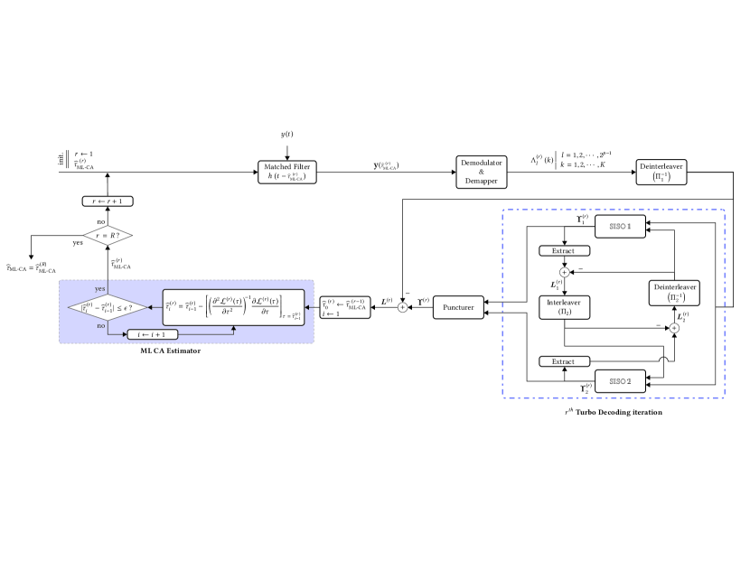
Figure 1: Flowchart of the new CA TD ML estimator.

VI Simulation Results

In this section, we provide some graphical representations of the new TD CA CRLBs for different modulation orders and different coding rates. We also analyze its computational complexity and compare it to that of the existing sum-product expectation-maximization (SP-EM) timing recovery algorithm [References]. The encoder is composed of two identical RSCs concatenated in parallel, having generator polynomials (1,0,1,1) and (1,1,0,1), and a systematic rate $R_{0}=\frac{1}{2}$ each. The output of the turbo encoder is punctured in order to achieve the desired code rate $R$. For the tailing bits, the size of the RSC encoders memory is fixed to $4$. We consider a root-raised-cosine (RRC) signal with roll-off factor $\alpha=0.2$. We also consider QPSK and 16-QAM, as two representative examples of square-QAM constellations, and two different coding rates, namely $R=\frac{1}{2}$ and $R=\frac{1}{3}$.

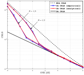
Figure 2: Comparison between the empirical and analytical CA CRLBs for different code rates, $R$, as function of the SNR: QPSK, rolloff $=0.2$.

We begin by verifying in Figs. 2 and 3 that the new analytical CA CRLBs coincide with their empirical counterparts obtained previously in [References] from exhaustive Monte-Carlo simulations. In fact, unlike our closed-form solution, an extremely large number of noisy observations was generated in [References] in order to find an empirical value for the expectation involved in the Fisher information (47). Hence, our new analytical expression corroborates these previous attempts to evaluate the underlying TD CA CRLBs empirically and allow their immediate evaluation for any square-QAM turbo-coded signal.

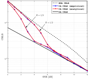
Figure 3: Comparison between the empirical and analytical CA CRLBs for different code rates, $R$, as function of the SNR: 16-QAM, rolloff $=0.2$.

As expected, we also see from both figures that the CA CRLBs are smaller than their NDA counterparts. This highlights the performance improvements that can be achieved by a coded system over an uncoded one by exploiting the information about the transmitted bits that is obtained from the SISO decoders. Additionally and most prominently, the CA CRLBs decrease rapidly and reach the DA CRLBs which are the best bounds ever one would be able to achieve if all the transmitted symbols were perfectly known to the receiver, hypothetically.
In the sequel, we also assess the performance of the new TD CA ML estimator using the normalized (by $T^{2}$) mean square error (NMSE) as a performance measure:

NMSE $$= \frac{1}{T^{2}}\frac{\sum_{m=1}^{M_{c}}\left(\widehat{\tau}_{\textrm{ML-CA}}^{[m]}-\bar{\tau}\right)^{2}}{M_{c}},$$ (99)

where $\widehat{\tau}_{\textrm{ML-CA}}^{[m]}$ is the estimate of $\tau$ generated from the $m^{th}$ Monte-Carlo run for $m=1,2\ldots,M_{c}$. In Figs. 4 and 5, we plot the NMSE of the new estimator for QPSK and 16-QAM transmissions obtained from $M_{c}=5000$ Monte-Carlo trials, and benchmark the resulting performance curves against the corresponding new CA CRLBs. To illustrate the performance advantage brought by CA estimation as compared to NCA estimation (from the algorithmic point of view), we also plot in the same figures the NMSE of the NDA TD ML estimator (94). Figs. 4 and 5 show that the potential estimation performance gains (attributed to the decoder’s assistance) made predictable now theoretically by the CA CRLBs can be achieved practically by the newly proposed CA ML estimator. More interestingly, the new estimator almost reaches the CA CRLB over the entire practical SNR range confirming thereby its statistical efficiency.

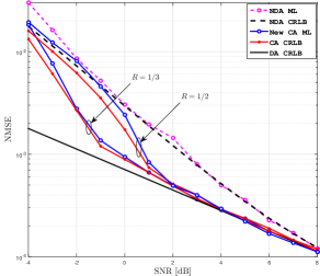
Figure 4: NMSE of the new CA ML estimator for different code rates, $R$, as function of the SNR: QPSK, rolloff $=0.2$.

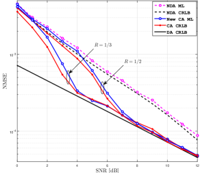
Figure 5: NMSE of the new CA ML estimator for different code rates, $R$, as function of the SNR: 16-QM, rolloff $=0.2$.

In the same figures, we can also observe unambiguously the effect of the coding rate, $R$, on CA estimation performance. Even though the same NMSE levels are achieved at relatively high SNRs for $R=\frac{1}{2}$ and $R=\frac{1}{3}$, the estimator performs quite differently for the two rates at the same SNR values. In fact, with smaller coding rates, more redundancy is introduced by the encoder and, hence, the decoder becomes more likely able to correctly detect the transmitted bits, thereby enhancing the estimation performance. Now, if we turn the tables and assess the effect of modulation order on estimation performance at the same coding rate, we observe without any surprise that it deteriorates with larger constellations at any given SNR level. This typical behavior was already observed in NDA estimation and, as a matter of fact, in any parameter estimation problem involving linearly-modulated signals. Indeed, when the modulation order increases, the inter-symbol distance decreases for normalized-energy constellations. As such, at the same SNR level, noise components have a relatively worse impact on symbol detection and parameter estimation in general.

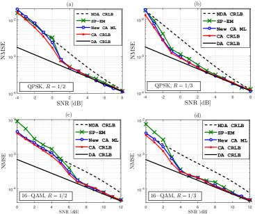
Figure 6: NMSE of the new CA ML estimator and SP-EM for different code rates and modulation orders, rolloff $=0.2$.

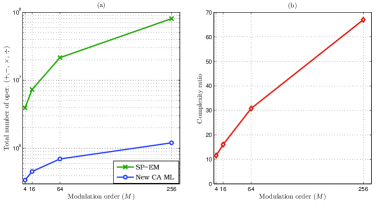
Figure 7: complexity of the new CA ML estimator and SP-EM for different code rates versus the modulation order: (a) total number of operations, and (b) complexity ratio.

Finally, we compare the new CA ML TDE to the existing SP-EM ML-based algorithm both in terms of estimation performance and computational complexity in Figs. 6 and 7, respectively.
In Fig. 6, even though both estimators perform nearly the same with QPSK signals over the entire SNR range, we observe with 16-QAM a clear advantage of the new CA ML TD estimator over SP-EM at low SNR levels. The superiority of the proposed estimator over SP-EM can be even better appreciated when it comes to computational complexity. In fact, we plot in Fig. 7-(a) the total number of operations (i.e., additions, multiplications, and divisions) required by both estimators versus the modulation order. There we can see that the new CA ML estimator entails much lower computational load. The ratio of complexities depicted in Fig. 7-(b) suggests, indeed, that the proposed estimator is about 30 and 70 times computationally less expensive than SP-EM for 64- and 256-QAM, respectively.

VII Conclusion

In this paper, we derived for the first time the closed-form expressions of the Cram r-Rao lower bounds for code-aided symbol timing estimation from turbo-coded square-QAM transmissions. The new CA CRLBs revealed the huge performance improvements in terms of timing recovery are achievable by exploiting the soft information delivered by SISO decoders at each turbo iteration. The new analytical CRLBs coincide exactly with their empirical counterparts established in previous pioneering works on the subject but from exhaustive Monte-Carlo simulations. We also developed a new code-aided ML time delay estimator that is able to achieve the potential performance gains made thoroughly and instantly predictable by the new closed-form CA CRLBs. The new estimator also exhibits a remarkable advantage in terms of computational complexity as compared to the most powerful ML-type algorithm that exists in the literature, namely SP-EM. Simulations results also show, as intuitively expected, that the CA estimation performance improves by decreasing the coding rate, i.e., increasing the amount of redundancy.

Appendix A

A.1) Proof of Lemma 1:
 
In order to find the pdfs of $u_{k}(\tau)$ and $v_{i}(\tau)$ defined in (37) and (38), respectively, and prove that they are two independent RVs, we define the following proper complex RV:

$$\!\!\!\!\!\!\!\!\!\!\!\!y_{k}(\tau) \!\!\!\!\triangleq\!\!\!\! \int_{-\infty}^{+\infty}\!\!\!y(t)~{}h(t-kT-\tau)dt~{}=~{}u_{k}(\tau)+jv_{k}(\tau),$$ (100)

which verifies $p\big{[}y_{k}(\tau)\big{]}=p\big{[}u_{k}(\tau),v_{k}(\tau)\big{]}$. Moreover, replacing $y(t)$ by its expression given by (4) in (100) and resorting to some easy algebraic manipulations, we obtain:

$$y_{k}(\tau)=\sqrt{E_{s}}\sum_{k^{\prime}=1}^{K}a(k^{\prime})\underbrace{\int_{-\infty}^{+\infty}\!\!\!h(x)h\big{(}x+[k^{\prime}-k]T\big{)}dt}_{g([k^{\prime}-k]T)}+~{}w_{k}(\tau),$$

where $w_{k}(\tau)$ is the filtered noise component, i.e.:

$$w_{k}(\tau)\triangleq\int_{-\infty}^{+\infty}\!\!\!w(t)h(t-kT-\tau)dt.$$ (101)

Recall that the shaping pulse $g(t)$ verifies the first Nyquist criterion stated in (6), i.e., $g([k^{\prime}-k]T)=\delta(k^{\prime}-k)$, thereby leading to:

$$y_{k}(\tau)=\sqrt{{E_{s}}}a(k)+~{}w_{k}(\tau).$$ (102)

Further, it can be verified from (101) that $w_{k}(\tau)$ is Gaussian distributed with zero-mean and variance $2\sigma^{2}$. Hence, the pdf of $y_{k}(\tau)$ conditioned on $a(k)$ is also Gaussian; i.e., $\forall c_{m}\in\mathcal{C}_{p}$ we have:

$$\!\!\!\!\!\!\!\!p\big{[}y_{k}(\tau)|a(k)=c_{m}\big{]} \!\!\!\!=\!\!\!\! {\frac{1}{2\pi\sigma^{2}}}\exp\!\left\{\!-{\frac{1}{2\sigma^{2}}}\big{|}y_{k}(\tau)\!-\!{\sqrt{E_{s}}}c_{m}\big{|}^{2}\!\right\}.$$

After expanding the modulus in the exponential argument, it can be easily shown that $\forall~{}c_{m}\in\mathcal{C}_{p}$ we have:

$$p\big{[}y_{k}(\tau)|a(k)=c_{m}\big{]} \!\!\!\!=\!\!\!\! {\frac{1}{2\pi\sigma^{2}}}{e^{-\frac{|y_{k}(\tau)|^{2}}{2\sigma^{2}}}}\Omega_{\tau}\big{(}c_{m},y(t)\big{)},$$ (103)

where $\Omega_{\tau}\big{(}c_{m},y(t)\big{)}$ is given in (22). Then, by averaging over all the constellation points in $\mathcal{C}_{p}$ and recalling the expression of $\bar{\Omega}_{k}(\tau)$ in (27), the pdf of $y_{k}(\tau)$ is obtained as:

$$p\big{[}y_{k}(\tau)\big{]}={\frac{1}{2\pi\sigma^{2}}}{e^{-\frac{|y_{k}(\tau)|^{2}}{2\sigma^{2}}}}\bar{\Omega}_{k}(\tau).$$ (104)

Finally, using the factorization of $\bar{\Omega}_{k}(\tau)$ obtained in (43) along with $|y_{k}(\tau)|^{2}=u_{k}^{2}(\tau)+v_{k}^{2}(\tau)$ and $\beta_{k}=\beta_{k,2p}\beta_{k,2p-1}$, it follows that:

$$\!p\big{[}y_{k}(\tau)\big{]} = {\frac{4\beta_{k,2p}\beta_{k,2p-1}}{2\pi\sigma^{2}}}{e^{-\frac{u_{k}^{2}(\tau)+v_{k}^{2}(\tau)}{2\sigma^{2}}}}F_{k,2p}\big{(}u_{k}(\tau)\big{)}F_{k,2p-1}\big{(}v_{k}(\tau)\big{.})$$

$$= \underbrace{{\frac{2\beta_{k,2p}}{\sqrt{2\pi\sigma^{2}}}}{e^{-\frac{u_{k}^{2}(\tau)}{2\sigma^{2}}}}\!F_{k,2p}\big{(}u_{k}(\tau)\big{)}}_{p[u_{k}(\tau)]}~{}\!\!\underbrace{{\frac{2\beta_{k,2p-1}}{\sqrt{2\pi\sigma^{2}}}}{e^{-\frac{v_{k}^{2}(\tau)}{2\sigma^{2}}}}\!F_{k,2p-1}\!\big{(}v_{k}(\tau)\big{)}}_{p[v_{k}(\tau)]}\!.$$

From the last equality, we obtain $p\big{[}y_{k}(\tau)\big{]}=p\big{[}u_{k}(\tau)\big{]}p\big{[}v_{k}(\tau)\big{]}$. But since from (100) we already have $y_{k}(\tau)=u_{k}(\tau)+jv_{k}(\tau)$, then we also have $p\big{[}y_{k}(\tau)\big{]}=p\big{[}u_{k}(\tau),v_{k}(\tau)\big{]}$. Therefore, it follows that $p\big{[}u_{k}(\tau),v_{k}(\tau)\big{]}=p\big{[}u_{k}(\tau)\big{]}p\big{[}v_{k}(\tau)\big{]}$, meaning that the two RVs $u_{k}(\tau)$ and $v_{k}(\tau)$ are actually independent and their distributions are, respectively, given by (51) and (52).
 
A.2) Statistical Independence of $u_{k}(\tau)$ and $\bm{\dot{}}u_{k}(\tau)$:
 
First, it follows from (100) that:

$$\!\!\!\!\!\!\!\!\!\!\!\!\bm{\dot{}}u_{k}(\tau) \!\!\!\!=\!\!\!\! \frac{\partial\Re\{y_{k}(\tau)\}}{\partial\tau}=-\int_{\mathbb{R}}\!\Re\big{\{}y(t)\big{\}}~{}\bm{\dot{}}h(t-kT-\tau)dt.$$ (105)

Again, we replace $y(t)$ by its expression given in (4) and then we use the fact that $\bm{\dot{}}{g}(.)$ is an odd function to show that:

$$\!\!\!\!\!\!\!\!\!\!\!\!\bm{\dot{}}u_{k}(\tau) \!\!\!\!=\!\!\!\! \sqrt{E_{s}}\sum\displaylimits_{k^{\prime}=1}^{K}\Re\big{\{}a(k^{\prime})\big{\}}\bm{\dot{}}g\big{(}[k-k^{\prime}]T\big{)}+\Re\big{\{}\bm{\dot{}}{w}_{k}(\tau)\big{\}},$$ (106)

where $\bm{\dot{}}w_{k}(\tau)$ is the derivative of $w_{k}(\tau)$ with respect to $\tau$, which is obtained by replacing $h(t-kT-\tau)$ by $-\bm{\dot{}}{h}(t-kT-\tau)$ back in (101). Recall also that $\bm{\dot{}}g(0)=0$ (since the maximum of $g(x)$ is located at $0$), leading to:

$$\!\!\!\!\!\!\!\!\!\!\!\!\bm{\dot{}}u_{k}(\tau) \!\!\!\!=\!\!\!\! \sqrt{E_{s}}\sum\displaylimits_{\mathclap{\begin{subarray}{c}k^{\prime}=1\\ k^{\prime}\neq k\end{subarray}}}^{K}\Re\big{\{}a(k^{\prime})\big{\}}\bm{\dot{}}g\big{(}[k-k^{\prime}]T\big{)}+\Re\big{\{}\bm{\dot{}}{w}_{k}(\tau)\big{\}}.$$ (107)

Recall also from (100) that $u_{k}(\tau)=\Re\{y_{k}(\tau)\}$ and, therefore, we have from (102) :

$$u_{k}(\tau)=\sqrt{E_{s}}\Re\big{\{}a(k)\big{\}}+\Re\big{\{}w_{k}(\tau)\big{\}}.$$ (108)

Notice from (107) that $\bm{\dot{}}u_{k}(\tau)$ involves the contribution of all the symbols except the $k^{th}$ one [i.e., $a(k)$] that is, in turn, the only one involved in $u_{k}(\tau)$ as seen from (108). Since the symbols are mutually independent, then in order to show the independence of $u_{k}(\tau)$ and $\bm{\dot{}}u_{k}(\tau)$, it suffices to show the independence of $w_{k}(\tau)$ and $\bm{\dot{}}{w}_{k}(\tau)$. These are actually two RVs that are obtained from linear transformations (i.e., integral and derivative) of the same Gaussian process $w(t)$ and, hence, they are also Gaussian distributed. Their cross-correlation is given by:

$$\!\!\mathbb{E}\left\{w_{k}(\tau)\bm{\dot{}}w_{k}(\tau)\right\}\! = \iint_{-\infty}^{+\infty}\!\!\!\!\mathbb{E}\big{\{}w(t_{1})w(t_{2})\big{\}}h(t_{1}-kT-\tau)\bm{\dot{}}h(t_{2}-kT-\tau)dt_{1}dt_{2}$$ (109)

$$= 2\sigma^{2}\!\iint_{-\infty}^{+\infty}\!\!\!\!\delta(t_{1}-t_{2})h(t_{1})\bm{\dot{}}h(t_{2})dt_{1}dt_{2}$$

$$= 2\sigma^{2}\bm{\dot{}}g(0)$$

$$= 0,$$

meaning that the two Gaussian-distributed RVs $w_{k}(\tau)$ and $\bm{\dot{}}{w}_{k}(\tau)$ are uncorrelated and, therefore, independent as well. Consequently, $u_{k}(\tau)$ and $\bm{\dot{}}u_{k}(\tau)$ are also independent.

Appendix B

Using the decomposition $\mathcal{C}_{p}=\widetilde{\mathcal{C}}_{p}\cup(-\widetilde{\mathcal{C}}_{p})\cup\widetilde{\mathcal{C}}_{p}^{*}\cup(-\widetilde{\mathcal{C}}_{p}^{*})$ and noticing that:

$$\Re\big{\{}\tilde{c}_{m}\big{\}}^{2}=\Re\big{\{}\!-\tilde{c}_{m}\!\big{\}}^{2}=\Re\big{\{}\tilde{c}^{*}_{m}\big{\}}^{2}=\Re\big{\{}\!-\tilde{c}^{*}_{m}\big{\}}^{2},~{}~{}~{}~{}\forall~{}\tilde{c}_{m}\in\widetilde{\mathcal{C}}_{p},$$

we rewrite (61) as follows:

$$\!\!\!\!\!\!\!\!\!\!\mathbb{E}\Big{\{}\!\Re\big{\{}a(k)\big{\}}^{2}\!\Big{\}} \!\!=\!\! \sum_{\tilde{c}_{m}\in\tilde{\mathcal{C}}_{p}}\!\!\!\Re\big{\{}\!\tilde{c}_{m}\!\big{\}}^{2}\Big{(}\!P\big{[}a(k)\!=\!\tilde{c}_{m}\big{]}\!+\!P\big{[}a(k)\!=\!-\tilde{c}_{m}\big{]}+P\big{[}a(k)\!=\!\tilde{c}^{*}_{m}\big{]}\!+\!P\big{[}a(k)\!=\!-\tilde{c}^{*}_{m}\big{]}\!\Big{)}.$$ (110)

Moreover, by using the explicit expressions of the symbols’ APPs given in (29)-(32), along with the identity $\cosh(x)+\cosh(y)=2\cosh(\frac{x+y}{2})\cosh(\frac{x-y}{2})$, we obtain:

$$Pr\big{[}a(k)\!=\!\tilde{c}_{m}\big{]}\!+\!Pr\big{[}a(k)\!=\!-\tilde{c}_{m}\big{]}\!+\!Pr\big{[}a(k)\!=\!\tilde{c}^{*}_{m}\big{]}\!+\!Pr\big{[}a(k)\!=\!-\tilde{c}^{*}_{m}\big{]}\!\!$$ (111)

$$\!\!\!\!\!\!\!\!\!\!\!\!\!\!\!\!\!\!\!\!\!\!\!\!\!\!\!\!\!\!\!\!\!\!\!\!\!\!\!\!\!\!\!\!\!\!\!\!\!\!\!\!\!\!\!\!\!\!\!\!\!\!\!\!\!\!\!\!\!\!\!\!=~{}2\beta_{k}\mu_{k,p}(\tilde{c}_{m})\!\left[{\cosh\left({\frac{L_{2p}(k)+L_{2p-1}(k)}{2}}\right)}\!+\!{\cosh\left({\frac{L_{2p}(k)-L_{2p-1}(k)}{2}}\right)}\right],$$

$$\!\!\!\!\!\!\!\!\!\!\!\!\!\!\!\!\!\!\!\!\!\!\!\!\!\!\!\!\!\!\!\!\!\!\!\!\!\!\!\!\!\!\!\!\!\!\!\!\!\!\!\!\!\!\!\!\!\!\!\!\!\!\!\!\!\!\!\!\!\!\!\!=~{}4\beta_{k}\mu_{k,p}(\tilde{c}_{m}){\cosh\left({\frac{L_{2p}(k)}{2}}\right)}{\cosh\left({\frac{L_{2p-1}(k)}{2}}\right)},$$

Now, plugging (111) back into (110), rewriting the sum over $\tilde{c}_{m}\in\tilde{\mathcal{C}}_{p}$ as a double sum over the counters $i$ and $n$ [where $\tilde{c}_{m}=(2i-1)d_{p}+j(2n-1)d_{p}$ as done in (39)], and using the decomposition in (40), it can be shown that:

$$\!\!\!\!\!\!\mathbb{E}\Big{\{}\Re\big{\{}a(k)\!\big{\}}^{2}\Big{\}} = 4\beta_{k}\sum_{i=1}^{2^{p-1}}\sum_{n=1}^{2^{p-1}}\Big{[}(2i-1)^{2}d_{p}^{2}\theta_{k,2p}(i)\theta_{k,2p-1}(n)\times{\cosh\left({\frac{L_{2p}(k)}{2}}\right)\cosh\left({\frac{L_{2p-1}(k)}{2}}\right)}\Big{]}$$

$$= 2\beta_{k,2p}{\cosh\left(\!{\frac{L_{2p}(k)}{2}}\!\right)}\sum_{i=1}^{2^{p-1}}(2i-1)^{2}d_{p}^{2}\theta_{k,2p}(i)\times 2\beta_{k,2p-1}{\cosh\left(\!{\frac{L_{2p-1}(k)}{2}}\!\right)}\sum_{n=1}^{2^{p-1}}\theta_{k,2p-1}(n),$$

where the decomposition $\beta_{k}=\beta_{k,2p}\beta_{k,2p-1}$ was used in the last equality as well. Moreover, it has been recently shown in [References, lemma 3] that for $q=2p$ and $2p-1$:

$$2\beta_{k,q}{\cosh\Big{(}\frac{L_{q}(k)}{2}\Big{)}}\displaystyle\sum_{n=1}^{2^{p-1}}\theta_{k,q}{(n)} = 1,$$ (113)

which is used back in (Appendix B) to obtain the following result:

$$\mathbb{E}\bigg{\{}\Re\big{\{}a(k)\!\big{\}}^{2}\bigg{\}} = \omega_{k,2p}.$$ (114)

References

- [1] 3GPP TS 36.211: 3rd Generation Partnership Project; Technical Specification Group Radio Access Network; Evolved Universal Terrestrial Radio Access (E-UTRA); Physical Channels and Modulation.
- [2] 3GPP TS 36.212 v8.0.0 (2007-09): “Multiplexing and channel coding (FDD) (Release 8)”. Available online at: http://www.3gpp.org/Highlights/LTE/LTE.htm
- [3] U. Mengali and A. N. D’andrea, Synchronization Techniques for Digital Receivers, New York: Plenum, 1997.
- [4] C. Berrou, “The ten-year old turbo codes are entering into service”, IEEE J. Commun. Mag., vol. 41, no. 8, pp. 110-116, Aug. 2003.
- [5] J. Riba, J. Sala, and G. Vazquez, “Conditional maximum likelihood timing recovery: Estimators and bounds,” IEEE Trans. Signal Process., vol. 49, no. 4, pp. 835-850, Apr. 2001.
- [6] W. Gappmair, S. Cioni, G. E. Corazza, and O. Koudelka, “Extended Gardner detector for improved symbol-timing recovery of M-PSK signals,” IEEE Trans. Commun., vol. 54 , no. 11, pp. 1923-1927, Nov. 2006.
- [7] W. Gappmair, “Self-noise performance of zero-crossing and Gardner synchronizers applied to one/two-dimensional modulation schemes,” Electron. Lett., vol. 40, no. 16, pp. 1010-1011, Aug. 2004.
- [8] M. Flohberger, W. Gappmair, and S. Cioni, “Two iterative algorithms for blind symbol timing estimation of M-PSK signals,” in Proc. of IEEE IWSSC, Tuscany, Italy, Sep. 2009, pp. 8-12.
- [9] W. Gappmair, “Symbol-timing recovery with modifed Gardner detectors,” in Proc. of 2nd International Symposium on Wireless Communication Systems, Siena, Italy, Sep. 2005, pp. 831-834.
- [10] W. Gappmair, S. Cioni, G. E. Corazza, and O. Koudelka, “A novel approach for symbol timing estimation based on the extended zero-crossing property ,” in Proc. of IEEE ASMS/SPSC, Livorno, Italy, Sept. 2014, pp. 59-65.
- [11] W. Gappmair and O. Koudelka, “Blind symbol timing recovery in the presence of IQ mismatch and DC offset,” presented at the 7th International Symposium on Communication Systems, Networks and Digital Signal Processing, Manchester, UK, 2010 .
- [12] P. Savazzi and P. Gamba, “Iterative symbol timing recovery for short burst transmission schemes,” IEEE Trans. Commun., vol. 56 , no. 10, pp. 1729-1736, Oct. 2008.
- [13] Y. C. Wu and E. Serpedin, “Unified analysis of a class of blind feedforward symbol timing estimators employing second-order statistics,” IEEE Trans. Wireless Commun., vol. 5, no. 4, pp. 737-742, Apr. 2006.
- [14] A. R. Nayak, J. R. Barry, G. Feyh, and S. W. McLaughlin, “Timing recovery with frequency offset and random walk: Cram r-Rao bound and a phase-locked loop postprocessor,” IEEE Trans. Commun., vol. 54, no. 11, pp. 2004-2013 Nov. 2006.
- [15] X. Man, H. Zahi, J. Yang, and E. Zhang, “Improved code-aided symbol timing recovery with large estimation range for LDPC-coded systems”, IEEE Commun. Lett., vol. 17, no. 5, pp. 1008-1011, Apr. 2013.
- [16] J. R. Barry, A. Kavcic, S. W. McLaughlin, A. Nayak, and W. Zeng, “Iterative timing recovery,” IEEE Signal Process. Mag., vol. 21, no. 1, pp. 89-102, Jan. 2004.
- [17] C. Herzet, V. Ramon, L. Vandendorpe, and M. Moeneclaey, “An iterative soft-decision-directed linear timing estimator,” in Proc. of IEEE Workshop on SPAWC, Rome, Italy, June 2003, pp. 55-59.
- [18] C. Herzet, V. Ramon, and L. Vandendorpe, “Turbo synchronization: a combined sum-product and expectation-maximization algorithm approach,” in Proc. IEEE SPAWC’05, New-York, USA, June 5-8, 2005, pp. 191-195.
- [19] C. Herzet, H. Wymeersch, M. Moeneclaey, and L. Vandendorpe, “On maximum-likelihood timing synchronization,” IEEE Trans. Commun., vol. 55, no. 6, pp. 1116-1119, June 2007.
- [20] A. Nayak, J. Barry, and S. McLaughlin, “Joint timing recovery and turbo equalization for coded partial response channels,” IEEE Trans. Mag., vol. 38, no. 5, pp. 2295-2297, Sept. 2003.
- [21] B. Mielczarek and A. Svensson, “Timing error recovery in turbo coded systems on AWGN channels,” IEEE Trans. Commun., vol. 50, pp. 1584-1592, Oct. 2002.
- [22] N. Wu, H. Wang, J. M. Kuang, and C. X. Yan, “Performance analysis of code-aided symbol timing recovery on AWGN channels,” IEEE Trans. Commun., vol. 59, no. 7, pp. 1975-1984, July 2011.
- [23] N. Noels, V. Lottici, A. Dejonghe, H. Steendam, M. Moeneclaey, M. Luise, and L. Vandendorpe, “A theoretical framework for soft information based synchronization in iterative (turbo) receivers,” EURASIP J. Wireless Commun. Netw., vol. 2005, no. 2, pp. 117-129, Apr. 2005.
- [24] J. Sun and M. C. Valenti, “Joint synchronization and SNR estimation for turbo codes in AWGN channels,” IEEE Trans. Commun., vol. 53, no. 7, pp. 1136-1144, July 2005.
- [25] C. Herzet, V. Ramon, and L. Vandendorpe, “A theoretical framework for iterative synchronization based on the sum-product and the expectation-maximization algorithms,” IEEE Trans. Signal Process., vol. 55, no. 5, pp. 1644 -1658, May 2007.
- [26] C. Herzet, N. Noels, V. Lottici, H. Wymeersch, M. Luise, M. Moeneclaey, and L. Vandendorpe, “Code-aided turbo synchronization,” Proc. IEEE, vol. 95, pp. 1255-1271, June 2007.
- [27] N. Noels, C. Herzet, A. Dejonghe, V. Lottici, H. Steendam, M. Moenedaey, M. Luke, and L. Vandendorpe, “Turbo synchronization: an EM algorithm interpretation,” in Proc. of IEEE ICC, Anchorage, Alaska, May 2003, pp. 2933-2937.
- [28] L. Zhang and A. Burr, “APPA symbol timing recovery scheme for turbo codes,” in Proc. of IEEE PIMRC’02, Lisbon, Portugal, Sept. 15-18, 2002, pp. 44-48
- [29] N. Noels, H. Wymeersch, H. Steendam, and M. Moeneclaey, “Carrier and clock recovery in (turbo) coded systems: Cramer-Rao bound and synchronizer performance,” EURASIP J. Appl. Signal Process., vol. 2005, no. 6, pp. 972-980, May 2005.
- [30] N. Noels, H. Wymeersch, H. Steendam, and M. Moeneclaey, “True Cramér-Rao bound for timing recovery from a bandlimited linearly modulated waveform with unknown carrier phase and frequency,” IEEE Trans. Comm., vol. 52, no. 3, pp. 473-383, Mar. 2004.
- [31] A. Masmoudi, F. Bellili, S. Affes, and A. St phenne, “Closed-form expressions for the exact Cram r-Rao bounds of timing recovery estimators from BPSK, MSK and square-QAM transmissions,” IEEE Trans. Signal Process., vol. 59, no. 6, pp. 2474-2484, June 2011.
- [32] L. Bahl, J. Cocke, F. Jelinek, and J. Raviv, “Optimal decoding of linear codes for minimizing symbol error rate”, IEEE Trans. Inf. Theory, vol. IT-20(2), no. 2, pp. 284-287, Mar. 1974.
- [33] F. Bellili, A. Methenni, and S. Affes, “Closed-form CRLBs for SNR estimation from turbo-coded BPSK-, MSK-, and square-QAM-modulated signals,” IEEE Trans. Signal Process., vol. 58, no. 15, pp. 4018-4033, Aug. 2014.
- [34] F. Bellili, A. Methenni, and S. Affes, “Closed-form CRLBs for CFO and phase estimation from turbo-coded square-QAM-modulated transmissions,” accepted for publication in IEEE Trans. Wireless Commun., DOI 10.1109/TWC.2014.2387855, to appear.
- [35] S. Mallat, A Wavelet Tour of Signal Processing, San Diego, CA: Academic, 1998.
- [36] S. M. Kay, Fundamentals of Statistical Signal Processing: Estimation Theory, Upper Saddle River, NJ: Prentice Hall, 1993.
- [37] T. J. Richardson, M. A. Shokrollahi, and R. L. Urbanke “Design of capacity-approaching irregular low-density parity-check codes”, IEEE Trans. Inform. Theory, vol. 47, no. 2, pp. 619-637, Feb. 2001.
- [38] M. M. Mansour and N. R. Shanbhag, “High throughput LDPC decoders,” IEEE Trans. Very Large Scale Integr. (VLSI) Syst., vol. 11, no. 6, pp. 976-996, Dec. 2003.