Stochastic Averaging and Sensitivity Analysis for Two Scale Reaction Networks

Abstract

In the presence of multiscale dynamics in a reaction network, direct simulation methods become inefficient as they can only advance the system on the smallest scale. This work presents stochastic averaging techniques to accelerate computations for obtaining estimates of expected values and sensitivities with respect to the steady state distribution. A two-time-scale formulation is used to establish bounds on the bias induced by the averaging method. Further, this formulation provides a framework to create an accelerated ‘averaged’ version of most single-scale sensitivity estimation methods. In particular, we propose a new lower-variance ergodic likelihood ratio method for steady state estimation and show how one can adapt it to accelerate simulations of multiscale systems. Lastly, we develop an adaptive “batch-means” stopping rule for determining when to terminate the micro-equilibration process.

I Introduction

Stochastic simulations have been an essential tool in analyzing reaction networks encountered in biology, catalysis, and materials growth. However, it is commonplace for reaction networks to exhibit a large disparity in time scales. These multi-scale stochastic reaction networks can impose an enormous computational burden in order to simulate them exactly. Exact techniques require computation of every reaction at the fastest time-scale, resulting in an exponentially growing load to observe dynamics on the slowest time-scale. Many works have attempted to develop approximate algorithms which allow faster computation with minimal loss of accuracy chatterjee_overview_2007 ; gillespie_approximate_2001 ; cao_avoiding_2005 ; cao_efficient_2006 ; rathinam_stiffness_2003 ; chatterjee_binomial_2005 ; tian_binomial_2004 ; salis_accurate_2005 ; samant_overcoming_2005 ; cao_slow-scale_2005 ; e_nested_2007 ; huang_strong_2014 ; kang_separation_2013 ; gupta_sensitivity_2014 .

One approach, which we refer to as Stochastic Averaging, takes its inspiration from classical singular perturbation theory of ordinary differential equations samant_overcoming_2005 ; cao_slow-scale_2005 ; e_nested_2007 ; huang_strong_2014 ; salis_accurate_2005 . The idea is that the fast dynamics come to quasi-equilibrium before the slow dynamics take effect, hence one may model the slow time scale dynamics with their averages against the steady-state distribution of the fast dynamics. By estimating the steady-state expectations of the slow propensities, one can then jump the system ahead to the next slow reaction and advance the time clock on the slow scale (skipping over needless computations of fast reactions).

In addition, one often desires the sensitivities of the system $S_{f}(\theta_{i})=\frac{\partial}{\partial\theta_{i}}\mathbb{E}_{{\boldsymbol{\theta}}}\{f(X(t))\}$ with respect to the reaction parameters $\theta_{i}$. The sensitivities give important insight into the system, indicating directions for gradient-descent type optimization as well as determining bounds for quantifying the uncertainty dupuis_path-space_2015 . Current techniques for estimating the sensitivities have large variance, requiring many more samples than those for estimating $\mathbb{E}_{{\boldsymbol{\theta}}}\{f(X)\}$ alone wolf_hybrid_2015 ; sheppard_pathwise_2012 ; wang_efficiency_2014 ; gupta_efficient_2014 . Thus computing sensitivities of multi-scale systems using single-scale techniques is often a computationally intractable problem.

In this work, we use results from Two-Time-Scale (TTS) Markov chains yin_continuous-time_2013 to show the error of stochastic averaging algorithms is inverse to the scale disparity in the system. As opposed to the previous approaches of transforming the system variables into auxiliary fast and slow variablese_nested_2007 ; huang_strong_2014 , we partition the underlying (discrete) state space and derive a singular perturbation expansion of the corresponding probability measure. The first order term can then be identified from computables of the averaged process, leading to a rigorous theoretical framework for applying singular perturbation averaging for stochastic systems.

Furthermore, this new formulation allows one to identify a macroscopic “averaged” reaction network on a reduced state space whose time-steps are on the macro (slow) time-scale. Thus, it provides a framework for applying single-scale sensitivity analysis techniques to the multi-scale system. Previous works have exploited similar model reduction techniques to estimate sensitivities via finite differencesgupta_sensitivity_2014 or a “truncated” version of a likelihood ratio estimatornunez_steady_2015 . This work develops an accelerated “Two-Time-Scale” version of the Likelihood Ratio (Girsanov Transform) method wang_efficiency_2014 ; plyasunov_efficient_2007 ; warren_steady-state_2012 ; glynn_likelihood_1990 for estimating system sensitivities of the multiscale system. The TTS-LR method computes sensitivity reweighting coefficients of the macro (reduced-state) process using a representation in terms of the steady-state sensitivities of the micro (fast) process. These micro-level sensitivities can in turn be computed online during the micro-equilibriation process. To this end, we propose a new lower-variance “Ergodic Likelihood Ratio” estimator for approximating steady-state sensitivities of single and multi-scale systems.

The outline of the remainder of the paper is as follows: Section II gives the theoretical basis of the paper. The Two-Time-Scale formulation is presented and error bounds are established. Section III then uses the TTS framework for the purpose of sensitivity analysis. A new ergodic likelihood ratio estimator is developed for single-scale steady-state sensitivity analysis, and is then adapted to the multiscale system. Section IV develops a batch-means stopping rule for determining when the micro-scale system has come to equilibrium. Numerical results are presented in Section V supporting the effectiveness of the methods presented. Concluding remarks are given in Section VI, and proofs of theorems are relegated to the Appendix.

II Formulation

II.1 Markov Chain Model of Reaction Networks

We briefly review the Markov chain model of reaction networks. While our motivation stems from chemical reaction networks, we note that much of the formulation carries over to general Markov chains on integer lattices.

Suppose we have $d$ species described by $X(t)=[X_{1}(t),X_{2}(t),\dots,X_{d}(t)]\in\mathcal{M}\subset\mathbb{Z}^{d}$ and $M$ reactions $r_{1},r_{2},\dots,r_{M}$. In stochastic reaction networks, one views $X(t)$ as a continuous-time Markov chain (CTMC) in the state space $\mathcal{M}$. When reaction $r$ fires at time $t$, the state is updated by the stoichiometric vector $\zeta_{r}$ so that $X(t)=X(t-)+\zeta_{r}$. Given the set of reaction parameters ${\boldsymbol{\theta}}=[\theta_{1},\theta_{2},\dots]$, one characterizes the probabilistic evolution of $X(t)$ by the propensity functions (intensity functions) $\lambda_{r}(x;{\boldsymbol{\theta}})$. The propensity functions are such that, given $X(t)=x$, the probability of one or more firing of reaction $r$ during time $(t,t+h]$ is $\lambda_{r}(x;{\boldsymbol{\theta}})h+o(h)$ as $h\to 0$; i.e. $\lambda_{r}(x;{\boldsymbol{\theta}})$ is the instantaneous rate/probability of reaction $r$ firing.

A common model for the propensities functions is that of mass-action kinetics. Under this assumption, the propensity functions are of the form

$$\lambda_{r}(x;{\boldsymbol{\theta}})=\theta_{r}\cdot b_{r}(x)=\theta_{r}\cdot\prod_{i=1}^{d}\frac{x_{i}!}{(x_{i}-\nu_{r,i})!}\mathbb{I}_{\{x-\nu_{r,i}\geq 0\}}$$ (1)

where $\nu_{r,i}$ is the number of molecules of species $i$ required for reaction $r$ to fire. Mass action kinetics assumes the system is well-mixed, so molecular interactions are proportional to their counts.

From the propensity functions $\lambda_{r}(x;{\boldsymbol{\theta}})$, one can construct the infinitesimal generator $Q=Q({\boldsymbol{\theta}})$ of the Markov chain. Viewed as an operator on functions $f$ of the state-space $\mathcal{M}$, we have

$$\left(Qf\right)(x)=\sum_{r=1}^{M}\lambda_{r}(x;{\boldsymbol{\theta}})\left(f(x+\zeta_{r})-f(x)\right)$$

For finite state-space $\mathcal{M}$ (bounded molecule counts), one may also view the generator $Q({\boldsymbol{\theta}})$ as a matrix. While the state-space is typically intractably large, the generator is sparse with only $M+1$ non-zero entries in each row,

$$Q(\boldsymbol{\theta})=\\ \bordermatrix{~{}&\dots&x+\zeta_{2}&\dots&x&\dots&x+\zeta_{1}&\dots\cr\vdots&~{}&~{}&~{}&~{}&~{}&~{}&~{}\cr x&\dots&\lambda_{2}(x;\boldsymbol{\theta})&\dots&-\lambda_{0}(x;\boldsymbol{\theta})&\dots&\lambda_{1}(x;\boldsymbol{\theta)}&\dots\cr\vdots&~{}&~{}&~{}&~{}&~{}&~{}&~{}}$$

where $\lambda_{0}(x;\boldsymbol{\theta})=\sum_{r=1}^{M}\lambda_{r}(x;\boldsymbol{\theta})$.

Writing $R_{r}(t)$ to be the counting process representing how many reactions of type $r$ have fired by the time $t$, we have that $X(t)=X(0)+\sum_{r=1}^{M}R_{r}(t)\zeta_{r}$. Using the random time change representation anderson_continuous_2011 ; ethier_markov_1986 , we write $X(t)$ as

$$\begin{aligned} X(t)=X(0)+\sum_{r=1}^{M}Y_{r}\left(\int_{0}^{t}\lambda_{r}(X(s);{\boldsymbol{\theta}})ds\right)\zeta_{r}\end{aligned}$$ (2)

where $Y_{r}(\cdot)$ are independent unit-rate Poisson processes. This representation is tremendously useful in conducting analysis of the trajectories. In particular, it leads to formulations of the Next-Reaction Method gibson_efficient_2000 ; anderson_modified_2007 and interpreting simulated trajectories in the path-space to allow for coupling paths rathinam_efficient_2010 ; anderson_efficient_2012 ; gupta_efficient_2014 as well as path-wise differentiation sheppard_pathwise_2012 ; wolf_hybrid_2015 .

When simulating exact trajectories (using any exact method; Direct SSA, Next-Reaction, etc), the propensity functions $\lambda_{r}(x;{\boldsymbol{\theta}})$ probabilistically determine both the time between reactions $\Delta t$ as well as the next reaction $r^{*}$ to fire. The likelihood that reaction $r_{k}$ is the next to fire is proportional to its propensity $\lambda_{k}(x;{\boldsymbol{\theta}})$; i.e. $\mathbb{P}_{{\boldsymbol{\theta}},x}\left\{r^{*}=r_{k}\right\}\propto\lambda_{k}(x;{\boldsymbol{\theta}})$. The time between reactions has an exponential distribution with the rate $\lambda_{0}(x;{\boldsymbol{\theta}})=\sum_{r=1}^{M}\lambda_{r}(x;{\boldsymbol{\theta}})$ ; i.e. $\Delta t\sim\mathcal{E}{{xp}}\left(\lambda_{0}(x;{\boldsymbol{\theta}})\right)$ with the mean $\mathbb{E}_{x,{\boldsymbol{\theta}}}\{\Delta t\}=1/\lambda_{0}(x,{\boldsymbol{\theta}})$.

Multi-scale dynamics occur when the propensity functions have large magnitude disparities. If $\lambda_{k}(x;{\boldsymbol{\theta}})\gg\lambda_{j}(x;{\boldsymbol{\theta}})$ for all $j\neq k$, then $\mathbb{P}\{r^{*}=r_{k}\}\approx 1$ and $\Delta t\sim\mathcal{E}{{xp}}\left(\lambda_{0}(x;{\boldsymbol{\theta}})\right)\approx\mathcal{E}{{xp}}\left(\lambda_{k}(x;{\boldsymbol{\theta}})\right)$. Thus, with a high probability the next reaction in an exact trajectory will be $r_{k}$ and the time clock will advance on the order of $1/\lambda_{k}(x;{\boldsymbol{\theta}})$. Such multi-scale networks then require an enormous number of computations to sample “slow” reactions and reach the required time horizon for the entire system to relax.

II.2 Two-Time-Scale Reaction Networks

We now consider reaction networks with two scales of dynamics. For further motivation and discussion of reaction networks with multiple time-scales, we refer readers to Refs. (13; 11; 12; 14) and references therein. We instead focus on our formulation for the separation of time-scales and the averaged process via the partitioning of the state space into “fast-classes”. Though analogous to the techniques of transforming the species variables into auxiliary fast/slow variables e_nested_2007 ; huang_strong_2014 or projecting to remainder spaces gupta_sensitivity_2014 , the direct partitioning of the state space will allow us to construct a singular perturbation expansion of the probability measure and establish the rate of convergence of such averaging methods. In addition, it provides a framework for applying Likelihood Ratio type sensitivity estimates to the averaged process as we shall see in the sequel.

Here, we assume that the disparity in the propensity functions results from magnitude disparities in the reaction parameters $\theta_{r}$. In order to illustrate the stiffness, we consider the reaction network

$$\begin{aligned} *\mathrel{\mathop{\rightleftharpoons}^{{\alpha}_{1}/\varepsilon}_{\mathrm{{\alpha}_{2}/\varepsilon}}}A&\qquad&A\mathrel{\mathop{\rightleftharpoons}^{{\beta}_{1}}_{\mathrm{{\beta}_{2}}}}B&\qquad&B\mathrel{\overset{{\beta}_{3}}{\rightharpoonup}}*\end{aligned}$$

where $\varepsilon\ll 1$ is a measure of the scale disparity (stiffness) between the fast reaction parameters ${{\boldsymbol{\alpha}}}=[\alpha_{1},\alpha_{2}]$ and the slow reaction parameters ${{\boldsymbol{\beta}}}=[\beta_{1},\beta_{2},\beta_{3}]$. As the stiffness parameter $\varepsilon\to 0$ the fast reactions ${{\boldsymbol{\alpha}}}$ dominate the system, resulting in the multi-scale computational problem described above.

In general, suppose a reaction network has species $[X_{1},X_{2},\dots,,X_{d}]$ and reactions $r_{1},\dots,r_{M}$. We shall assume that the propensity functions $\lambda_{r}(x;{\boldsymbol{\theta}})$ are of the form (1) (mass-action kinetics, though other forms may also be treated), and that each reaction is indexed by its own reaction parameter $\theta_{r}$. As in the illustrating example, we assume that there is a scale disparity in the reaction parameters between a set of “fast reactions” and a set of “slow reactions”. Thus we can write ${\boldsymbol{\theta}}=[\theta_{1},\dots,\theta_{M}]=[{{\boldsymbol{\alpha}}}/\varepsilon,{{\boldsymbol{\beta}}}]$, where ${{\boldsymbol{\beta}}}=[\beta_{1},\beta_{2},\dots,\beta_{M_{s}}]$ are the slow reaction parameters, $\varepsilon\ll 1$ is the stiffness parameter, and ${{\boldsymbol{\alpha}}}=[\alpha_{1},\dots,\alpha_{M_{f}}]$ are the underlying (rescaled) reaction parameters for the fast reactions.

To ease referencing, we will often index reactions and propensity functions directly by their reaction parameter. E.g., $r_{\beta_{i}}$ is the reaction with reaction parameter $\beta_{i}$ and propensity function $\lambda_{\beta_{i}}(x;{\boldsymbol{\theta}})=\lambda_{\beta_{i}}(x;{{\boldsymbol{\beta}}})=\beta_{i}b_{\beta_{i}}(x)$ (where $b_{\beta_{i}}$ is given by (1)). For the fast reactions $\alpha_{i}$, we use $\lambda^{\varepsilon}_{\alpha_{i}}(x;{\boldsymbol{\theta}})=\lambda^{\varepsilon}_{\alpha_{i}}(x;{{\boldsymbol{\alpha}}})=({\alpha_{i}}/{\varepsilon})b_{\alpha_{i}}(x)$ to denote the exact propensity function and $\lambda_{\alpha_{i}}(x;{\boldsymbol{\theta}})=\alpha_{i}\ b_{\alpha_{i}}(x)$ to denote the rescaled version.

Let $X^{\varepsilon}(t)$ denote the Markov chain determined by the exact propensity functions $\lambda^{\varepsilon}_{\alpha}(x;{\boldsymbol{\theta}})$ and $\lambda_{\beta}(x;{\boldsymbol{\theta}})$. We can write the generator $Q^{\varepsilon}=Q^{\varepsilon}({{\boldsymbol{\alpha}}},{{\boldsymbol{\beta}}})$ of the exact process as before, and observe that

$$\begin{aligned} (Q^{\varepsilon}f)(x)&=\sum_{r=1}^{M}\lambda_{r}(x;{\boldsymbol{\theta}})\left(f(x+\zeta_{r})-f(x)\right)\\ &=\frac{1}{\varepsilon}\sum_{i=1}^{M_{f}}\lambda_{\alpha_{i}}(x;{{\boldsymbol{\alpha}}})\left(f(x+\zeta_{\alpha_{i}})-f(x)\right)\\ &\qquad+\sum_{j=1}^{M_{s}}\lambda_{\beta_{j}}(x;{{\boldsymbol{\beta}}})\left(f(x+\zeta_{\beta_{j}})-f(x)\right)\\ &=\left(\left[\frac{1}{\varepsilon}\widetilde{Q}({{\boldsymbol{\alpha}}})+\widehat{Q}({{\boldsymbol{\beta}}})\right]f\right)(x)\end{aligned}$$ (3)

where $\widehat{Q}({{\boldsymbol{\beta}}})$ is the generator of the chain under only the slow dynamics (determined by slow reactions $r_{\beta}$), and $\widetilde{Q}({{\boldsymbol{\alpha}}})$ is the generator of the chain under only the fast dynamics (with the rescaled propensity functions $\lambda_{\alpha}(x;{{\boldsymbol{\alpha}}})$). Thus we have a decomposition of the generator into the fast and slow dynamics, $Q^{\varepsilon}({{\boldsymbol{\alpha}}},{{\boldsymbol{\beta}}})=(1/\varepsilon)\widetilde{Q}({{\boldsymbol{\alpha}}})+\widehat{Q}({{\boldsymbol{\beta}}})$ One can also view the generator $Q^{\varepsilon}({{\boldsymbol{\alpha}}},{{\boldsymbol{\beta}}})=(1/\varepsilon)\widetilde{Q}({{\boldsymbol{\alpha}}})+\widehat{Q}({{\boldsymbol{\beta}}})$ as a matrix. In this case, we can write the element corresponding to the rate of transition from state $x$ to state $y$ as

$$\left[\widetilde{Q}(\boldsymbol{\alpha})\right]_{x,y}=\left\{\begin{array}[]{*1{>{\displaystyle}c }l}-\sum_{\alpha\in\boldsymbol{\alpha}}\lambda_{\alpha}(x)&\quad x=y\\ \sum_{\alpha:r_{\alpha}(x)=y}\lambda_{\alpha}(x)&\quad x\neq y\end{array}\right.$$

and similarly for $\left[\widehat{Q}(\boldsymbol{\beta})\right]_{x,y}$.

As $\varepsilon\to 0$ only the fast reactions $r_{\alpha}$ fire, and so we define an equivalence relation on states $s\in\mathcal{M}$, by $s_{i}\leftrightarrow s_{j}$ if they are mutually accessible through only fast reactions. This defines a partition of the state space $\mathcal{M}$ into “fast-classes” $\mathcal{M}_{k}$ which are by construction the invariant (irreducible) classes of $\mathcal{M}$ under $\widetilde{Q}({{\boldsymbol{\alpha}}})$; e.g.

$$\mathcal{M}=\bigcup_{k=1}^{N_{C}}\mathcal{M}_{k}=\left\{x^{(1)}_{1},x^{(1)}_{2},\dots,x^{(1)}_{m_{1}},x^{(2)}_{1},\dots,x^{(2)}_{m_{2}},\dots\right\}$$

where ${N_{C}}$ are the number of invariant “fast-classes”, and $m_{k}=\big{|}\mathcal{M}_{k}\big{|}$ is the number of states inside fast-class $\mathcal{M}_{k}$. For ease of presentation, in the present discussion we shall assume the state space is finite.

Assumption II.1 (Finite State Space).

The state space $\mathcal{M}$ is finite, such that $|\mathcal{M}|=m$. Thus the number of fast classes ${N_{C}}<\infty$ and the number of states in each fast-class $m_{k}<\infty$, so that $m=m_{1}+m_{2}+\dots+m_{N_{C}}$.

Assumption II.1 is made only to simplify the discussion. One may also treat the infinite state case with some mild additional conditions on $\widetilde{Q}({{\boldsymbol{\alpha}}})$ and $\widehat{Q}({{\boldsymbol{\beta}}})$ to ensure non-explosiveness and ergodicity of the underlying (rescaled) chainyin_continuous-time_2013 . In addition, we shall impose the following assumption.

Assumption II.2 (Recurrent States).

Each state of $\mathcal{M}$ is recurrent, so that there are no absorbing/transient states.

Assumption II.2 is satisfied if, for example, all reactions are reversible (or often times if only the fast reactions are reversible). One may also treat the case with transient/absorbing classes with some additional stability assumptions to ensure the fast dynamics decay to steady-state; see Section 4.4 of Ref. (20) for more details.

Under Assumption II.2, we can reorder the state space so that $\widetilde{Q}({{\boldsymbol{\alpha}}})={\operatorname{diag}}[\widetilde{Q}^{(1)}({{\boldsymbol{\alpha}}}),\widetilde{Q}^{(2)}({{\boldsymbol{\alpha}}}),\dots,\widetilde{Q}^{({N_{C}})}({{\boldsymbol{\alpha}}})]$ is block-diagonal. Here, one can view the generators $\widetilde{Q}^{(k)}({{\boldsymbol{\alpha}}})$ as the restriction of $\widetilde{Q}({{\boldsymbol{\alpha}}})$ to the (irreducible) fast-class $\mathcal{M}_{k}$ (fast-only dynamics when $X(0)\in\mathcal{M}_{k}$). In light of the finite state-space and positive recurrence, each $\widetilde{Q}^{(k)}({{\boldsymbol{\alpha}}})$ is ergodic and has a stationary (steady-state) probability measure $\widetilde{\pi}^{(k)}=\widetilde{\pi}^{(k)}({{\boldsymbol{\alpha}}})$ such that $\widetilde{\pi}^{(k)}\widetilde{Q}^{(k)}=\boldsymbol{0}$ (with $\widetilde{\pi}^{(k)},\boldsymbol{0}$ interpreted as row vectors).

Using the above formulation, we can restate the averaging principle e_nested_2007 ; cao_slow-scale_2005 ; samant_overcoming_2005 ; huang_strong_2014 ; kang_separation_2013 ; gupta_sensitivity_2014 as follows. For small $\varepsilon$ and $X(0)\in\mathcal{M}_{k}$, $X^{\varepsilon}(\cdot)$ will relax to its steady-state distribution $\pi^{(k)}$ on the micro time-scale $\varepsilon t$ before any slow reaction fires (on the macro time scale $t$). Thus, one can use the stationary average of the slow propensity functions

$$\lambda_{\beta_{j}}\left(X\left(t\right);{{\boldsymbol{\beta}}},X(0)\in\mathcal{M}_{k}\right)\\ \sim\overline{\lambda}_{\beta_{j}}\left(\mathcal{M}_{k};{\boldsymbol{\theta}}\right)\overset{\Delta}{=}\mathbb{E}_{\widetilde{\pi}^{(k)}({{\boldsymbol{\alpha}}})}\left\{\lambda_{\beta_{j}}\left(X;{{\boldsymbol{\beta}}}\right)\right\}$$ (4)

to determine the distribution of time until the next slow reaction as well as the probabilities for the next slow reaction being $r_{\beta_{j}}$. These can then be used to simulate a trajectory of the slow (macro-scale) process. We shall further develop this idea more precisely in the remainder.

Write $m=\big{|}\mathcal{M}\big{|}$, and $m_{k}=\big{|}\mathcal{M}_{k}\big{|}$ as before, so that $Q^{\varepsilon}({\boldsymbol{\theta}}),\widetilde{Q}({{\boldsymbol{\alpha}}}),\widehat{Q}({{\boldsymbol{\beta}}})\in\mathbb{R}^{m\times m}$, $\widetilde{Q}^{(k)}({{\boldsymbol{\alpha}}})\in\mathbb{R}^{m_{k}\times m_{k}}$, and $\pi^{(k)}({{\boldsymbol{\alpha}}})\in\mathbb{R}^{1\times m_{k}}$. Write $\widetilde{\pi}({{\boldsymbol{\alpha}}})={\operatorname{diag}}\left[\widetilde{\pi}^{(1)},\widetilde{\pi}^{(2)},\dots,\widetilde{\pi}^{({N_{C}})}\right]\in\mathbb{R}^{{N_{C}}\times m}$. Write $\boldsymbol{1}_{m_{k}}$ for $[1,1,\dots,1]^{\prime}\in\mathbb{R}^{m_{k}\times 1}$ and $\widetilde{\boldsymbol{1}}={\operatorname{diag}}\left[\boldsymbol{1}_{m_{1}},\boldsymbol{1}_{m_{2}},\dots,\boldsymbol{1}_{m_{N_{C}}}\right]$

With $\widetilde{\pi}({{\boldsymbol{\alpha}}})$ describing the limit behavior inside each fast-class on the micro time scale, one can then consider the distribution of the exact system $X^{\varepsilon}$ on the macro time scale. Heuristically, one expects a trajectory to enter a fast-class of states $\mathcal{M}_{k_{1}}$ and quickly iterate through many fast reactions until the distribution of the trajectory reaches the steady-state $\widetilde{\pi}^{(k_{1})}$. Eventually, a slow reaction will fire to move the trajectory to a new fast-class $\mathcal{M}_{k_{2}}$ (see Figure 1). Indeed, Writing

$$\begin{aligned} \overline{Q}=\overline{Q}({{\boldsymbol{\alpha}}},{{\boldsymbol{\beta}}})\overset{\Delta}{=}\left[\widetilde{\pi}({{\boldsymbol{\alpha}}})\cdot\widehat{Q}({{\boldsymbol{\beta}}})\cdot\widetilde{\boldsymbol{1}}\right]\in\mathbb{R}^{{N_{C}}\times{N_{C}}},\end{aligned}$$ (5)

we see that $\overline{Q}$ is itself a generator of an “averaged” CTMC reaction network, whose “states” correspond to fast-classes $\mathcal{M}_{k}$. Write $\overline{X}(t)$ for the “averaged” process generated by $\overline{Q}$. Together, $\overline{Q}$ and $\overline{X}(t)$ describe the limit (as $\varepsilon\to 0$) of the average rate that the exact process $X^{\varepsilon}(t)$ moves between the fast-classes $\left\{\mathcal{M}_{k}\right\}_{k=1}^{N_{C}}$ via slow reactions.

Furthermore, we can identify the elements of $\overline{Q}$ from the steady-state averages of the slow propensity functions. First, note that every slow reaction carries each fast class to a unique new fast-class; that is, if $x\leftrightarrow y$ and $\lambda_{\beta}(x),\lambda_{\beta}(y)>0$, then $r_{\beta}(x)\leftrightarrow r_{\beta}(y)$. Thus, $r_{\beta}(\mathcal{M}_{k})$ is well-defined. Then, using the form of $\widehat{Q}$ together with (5), we have

$$\begin{aligned} \overline{Q}_{k_{1},k_{2}}&=\sum_{\begin{subarray}{c}\beta\in{{\boldsymbol{\beta}}}\\ r_{\beta}(\mathcal{M}_{k_{1}})=\mathcal{M}_{k_{2}}\end{subarray}}\overline{\lambda}_{\beta}(\mathcal{M}_{k_{1}};{\boldsymbol{\theta}})\end{aligned}$$ (6)

for $k_{1}\neq k_{2}$, and similarly we see that

$$\overline{Q}_{k_{1},k_{1}}=-\sum_{\beta\in{{\boldsymbol{\beta}}}}\overline{\lambda}_{\beta}(\mathcal{M}_{k_{1}};{\boldsymbol{\theta}})\overset{\Delta}{=}-\overline{\lambda}_{\beta_{0}}(\mathcal{M}_{k_{1}};{\boldsymbol{\theta}}).$$ (7)

With this formulation, we see that generator $\overline{Q}$ corresponds to a meta “macro” reaction network with the state-space $\overline{\mathcal{M}}=\left\{\mathcal{M}_{1},\mathcal{M}_{2},\dots,\mathcal{M}_{N_{C}}\right\}$, reactions $\{r_{\beta}:\beta\in{{\boldsymbol{\beta}}}\}$ and propensities $\{\overline{\lambda}_{\beta}(\overline{X};{\boldsymbol{\theta}}):\beta\in{{\boldsymbol{\beta}}}\}$. Figure  1 depicts such a macro chain for the macro process $\overline{X}(t)$.

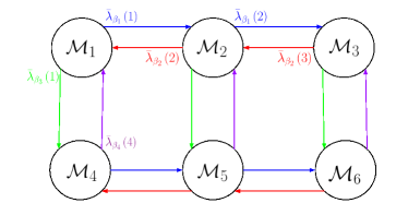
Figure 1: A depiction of the macro chain of a Two-Time-Scale Reaction Network. Each fast-class $\mathcal{M}_{k}$ is an equivalence class of states accessible by fast-reactions $r_{\alpha}$. Slow reactions $r_{\beta}$ carry each fast-class to a unique new fast-class. The averaged system $\overline{X}(t)$ forms a meta “macro” Markov chain among fast-classes with propensities $\overline{\lambda}_{\beta}\left(\overline{X};{{\boldsymbol{\beta}}},\widetilde{\pi}({{\boldsymbol{\alpha}}})\right)$.

If we can estimate the average slow-propensities $\widehat{\overline{\lambda}}_{\beta}(\mathcal{M}_{k};{\boldsymbol{\theta}})$ within each fast-class (say, through ergodic time averages of the fast-only process), then one can simulate a trajectory of the macro process $\overline{X}(t)$ from these average propensities using any single-scale Monte Carlo simulation (e.g. Direct SSA, Next-Reaction, etc). Furthermore, if one is ultimately concerned with estimating $\mathbb{E}_{{\boldsymbol{\theta}}}\left\{f\left(X^{\varepsilon}(t)\right)\right\}$ for some observable (quantity of interest) $f:\mathcal{M}\to\mathbb{R}$, then one can define an augmented functional $\overline{f}$ on $\overline{\mathcal{M}}$ by

$$\overline{f}\left(\mathcal{M}_{k};{{\boldsymbol{\alpha}}}\right)\overset{\Delta}{=}\mathbb{E}_{\widetilde{\pi}^{(k)}({{\boldsymbol{\alpha}}})}\left\{f(X)\right\}=\sum_{x\in\mathcal{M}_{k}}f(x)\widetilde{\pi}^{(k)}_{x}({{\boldsymbol{\alpha}}})$$ (8)

It shall be shown that $\mathbb{E}_{{\boldsymbol{\theta}}}\left\{\overline{f}(\overline{X}(t))\right\}\approx\mathbb{E}_{{\boldsymbol{\theta}}}\left\{f\left(X^{\varepsilon}(t)\right)\right\}$ for large enough $t$ and sufficiently small $\varepsilon$.

To illustrate how one can implement the averaging scheme to generate macro-trajectories, we present the following TTS vlersion of the Direct SSA (since it is the most succinct to write). In this case, the TTS SSA is essentially the same algorithm as in Refs. (11), (9). However, we emphasize that the same method can be used to create a TTS version of any exact method defined by the propensity functions. In particular, one can just as easily construct an analogous TTS Next-Reaction type algorithm rathinam_efficient_2010 ; anderson_efficient_2012 ; anderson_modified_2007 for tightly coupled trajectories.

Algorithm 1 (TTS-SSA).

To simulate a trajectory of the macro-process $\overline{X}(T)$ until macro time-horizon $T_{final}$:

1. Initialize $x$ at a macro time $T$; $x\in\mathcal{M}_{k}$ for some (unknown) $k$

2. Simulate the fast-only reaction network ${\widetilde{Q}^{(k)}}(\boldsymbol{\alpha})$ until time-averages of observable $f$ and slow propensities $\lambda_{\beta}$ relax to steady-state :

   $$\frac{1}{t}\int_{0}^{t}f\left({\widetilde{X}^{(k)}}(s)\right)ds \to \mathbb{E}_{{\widetilde{\pi}^{(k)}({{\boldsymbol{\alpha}}})}}\left\{f(\widetilde{X})\right\}\equiv{\overline{f}(k)}$$

   $$\frac{1}{t}\int_{0}^{t}\lambda_{{\beta}}\left({\widetilde{X}^{(k)}}(s);\boldsymbol{{\beta}}\right)ds \to \mathbb{E}_{{\widetilde{\pi}^{(k)}({{\boldsymbol{\alpha}}})}}\left\{\lambda_{\beta}\left(\widetilde{X};\boldsymbol{\beta}\right)\right\}$$

   $$\equiv {\overline{\lambda}_{\beta}(k;{\boldsymbol{\theta}})}$$

3. Observe terminal state ${\widetilde{x}^{(k)}}\sim{\widetilde{\pi}^{(k)}}$. Compute ${\overline{\lambda}_{\beta_{0}}}=\sum_{j=1}^{Ms}{\overline{\lambda}_{\beta_{j}}}$

4. Sample time to next slow reaction : $\Delta T\sim\mathcal{E}{{xp}}({\overline{\lambda}_{\beta_{0}}})$

5. Sample next slow rxn to fire ${\beta^{*}}\sim 1/{\overline{\lambda}_{\beta_{0}}}\left[{\overline{\lambda}_{\beta_{1}}},\dots,{\overline{\lambda}_{\beta_{Ms}}}\right]$

6. Update macro time $T\leftarrow T+\Delta T$ and move to the next fast class by taking $x={\widetilde{x}^{(k)}}+{\zeta_{\beta^{*}}}$

7. Return to (1) until macro time horizon $T_{final}$ is reached

II.3 Convergence and Error Bounds

Here we use the above formulation of stiff networks to establish convergence results and error bounds for the averaged process obtained by Algorithm 1. They are largely obtained by applying results from Ref. (20) to the Two-Time-Scale Markov chain developed above. We give the statements below and defer to the Appendix for the proofs.

From the exact chain $X^{\varepsilon}(t)$, define a stochastic process $\overline{X^{\varepsilon}}(t)$ taking values in $\overline{\mathcal{M}}=\{\mathcal{M}_{1},\dots,\mathcal{M}_{N_{C}}\}$ by $\overline{X^{\varepsilon}}(t)=\mathcal{M}_{k}$ for $X^{\varepsilon}(t)\in\mathcal{M}_{k}$. Note that $\overline{X^{\varepsilon}}(t)$ is not, in general, a Markov chain. However, one expects that as $\varepsilon\to 0$, the process $\overline{X^{\varepsilon}}(t)$ converges to $\overline{X}(t)$ in some sense.

Proposition II.3 (Weak Convergence).

Under Assumptions II.2 and II.1, as $\varepsilon\to 0$, $\overline{X^{\varepsilon}}(\cdot)$ converges weakly to $\overline{X}(\cdot)$ in the Skorohod space $\mathcal{D}([0,T];\overline{\mathcal{M}})$ for any time horizon $T$.

The above proposition establishes weak convergence of the projection (onto fast-classes) of the exact system $X^{\varepsilon}$ to the averaged meta system $\overline{X}$ as $\varepsilon\to 0$. This is essentially the same result as established in Ref. (13), where the authors instead consider the disparity of the propensities as the system size (molecule count) $N\to\infty$. In both formulations, one selects a reference scale and then examines limit behavior against the reference scale as the disparity increases ($\varepsilon\to 0$ or $N\to\infty$). However, in practice one implements the averaging procedure to approximate a system with a fixed, positive scale disparity. Naturally, one is then concerned about the induced error from the averaging approximation.

Write $\overline{p}_{T}=\overline{p}_{T}(\overline{X};{{\boldsymbol{\alpha}}},{{\boldsymbol{\beta}}})$ for the probability measure (on $\overline{\mathcal{M}}$) induced by the averaged process $\overline{X}$ at time $T$. At the end of a TTS simulation, one obtains a terminal state $X(T)=x\sim p^{0}_{T}=p^{0}_{T}(X;{{\boldsymbol{\alpha}}},{{\boldsymbol{\beta}}})$, where $p^{0}_{T}$ is the probability measure on $\mathcal{M}$ induced by the last state observed from the terminal fast-class. Thus, $p^{0}_{T}$ is determined by $\overline{p}_{T}$ and $\widetilde{\pi}({{\boldsymbol{\alpha}}})$. Write $p^{\varepsilon}_{T}=p^{\varepsilon}(X^{\varepsilon};{{\boldsymbol{\alpha}}},{{\boldsymbol{\beta}}})$ for the probability measure on $\mathcal{M}$ induced from the exact process $X^{\varepsilon}$. Since $p^{\varepsilon}_{T}$ is the distribution we would see from an exact simulation, and $p^{0}_{T}$ is the distribution from the TTS simulation, the question becomes: What is the error of $p^{0}_{T}$ from $p^{\varepsilon}_{T}$? One can take a singular perturbation expansion of $p^{\varepsilon}_{T}$ in terms of $\varepsilon$ and identify the leading term as $p^{0}_{T}$ to obtain the following result.

Theorem II.4 (Error in Probability).

Let $\widetilde{\kappa}=-\frac{1}{2}\max\left\{\operatorname{Re}(\nu):\nu\text{ is a non-zero eigenvalue of a }\widetilde{Q}^{(k)}\right\}$. Then under Assumptions II.1, II.2, we have

$$\begin{aligned} \|p^{0}_{T}-p^{\varepsilon}_{T}\|\leq O\left(\varepsilon+\exp\left\{-\widetilde{\kappa}T/\varepsilon\right\}\right)\end{aligned}$$ (9)

where $\|\cdot\|$ denotes the $l_{2}$ norm.

In Theorem II.4, $\widetilde{\kappa}$ is the slowest rate of convergence of $\widetilde{Q}^{(k)}$ to the steady-state $\widetilde{\pi}^{(k)}$ among all fast-classes $\mathcal{M}_{k}$. Thus, as long as the macro time horizon $T$ is large enough to ensure the fast dynamics have relaxed to steady state ($T>-\varepsilon/\widetilde{\kappa}\log(\varepsilon)$), then the error becomes $\|p^{0}_{T}-p^{\varepsilon}_{T}\|\leq O(\varepsilon)$.

Writing $\pi^{0}({{\boldsymbol{\alpha}}},{{\boldsymbol{\beta}}})$ for the stationary distribution corresponding to the TTS probability measure $p^{0}_{T}({{\boldsymbol{\alpha}}},{{\boldsymbol{\beta}}})$, it is not hard to see that $\pi^{0}({{\boldsymbol{\alpha}}},{{\boldsymbol{\beta}}})=\overline{\pi}\cdot\widetilde{\pi}$, the product of the steady-state distribution between fast-classes $\overline{\pi}({{\boldsymbol{\alpha}}},{{\boldsymbol{\beta}}})$ and the steady-state distribution within fast-classes $\widetilde{\pi}({{\boldsymbol{\alpha}}})$. Write $\pi^{\varepsilon}$ for the steady-state distribution corresponding to the exact process generated by $Q^{\varepsilon}$. Then using Theorem II.4 and exponential convergence to the steady state, we obtain the following error bounds.

Corollary II.5 (Error in Expectation).

Under Assumptions II.1 and II.2, $\|\pi^{0}-\pi^{\varepsilon}\|\leq O(\varepsilon)$ and $\|\pi^{0}-p^{\varepsilon}_{T}\|\leq O(\varepsilon)$ for sufficiently large $T$. Thus, for all bounded functions $f$ on the state space $\mathcal{M}$,

$$\begin{aligned} \left|\mathbb{E}_{\overline{p}_{T}}\left\{\overline{f}(\overline{X}(T))\right\}\right.&-\left.\mathbb{E}_{p^{\varepsilon}_{T}}\left\{f(X^{\varepsilon}(T))\right\}\right|\leq\\ &\|f\|_{\infty}\|p^{0}_{T}-p^{\varepsilon}_{T}\|\leq O(\varepsilon)\\ \left|\mathbb{E}_{\overline{\pi}}\left\{\overline{f}(\overline{X})\right\}\right.&-\left.\mathbb{E}_{\pi^{\varepsilon}}\left\{f(X^{\varepsilon})\right\}\right|\leq\\ &\|f\|_{\infty}\|\pi^{0}-\pi^{\varepsilon}\|\leq O(\varepsilon)\end{aligned}$$ (10)

Corollary II.5 is of great practical use, as it says that the expected value of the macro-process $\overline{X}(T)$ with macro-observable $\overline{f}:\overline{\mathcal{M}}\to\mathbb{R}$ provides an $O(\varepsilon)$ estimate of the expected value of the exact system $X^{\varepsilon}(T)$ with observable $f:\mathcal{M}\to\mathbb{R}$. Since we can use TTS algorithms (such as Algorithm 1) to quickly generate trajectories of $\overline{X}(T)$ while estimating the macro-observable $\overline{f}(\mathcal{M}_{k})$ at each state along the way, this provides a method to very quickly generate estimates of $\mathbb{E}_{p^{\varepsilon}_{T}}\left\{f(X^{\varepsilon}(T))\right\}$ with at most $O(\varepsilon)$ bias. As $\varepsilon\to 0$, the bias decreases linearly while the computational savings increase as $O(1/\varepsilon)$.

III Two Time Scale Sensitivity Analysis

Computing the system sensitivities $S_{f,T}(\theta_{i})\overset{\Delta}{=}\frac{\partial}{\partial\theta_{i}}\mathbb{E}_{\boldsymbol{\theta}}\left\{f(X(T))\right\}$ with respect to reaction parameters $\theta_{i}\in{\boldsymbol{\theta}}$ provides great insight into the model. As such, numerous works have constructed and analyzed methods to estimate the sensitivities from sample trajectories of the system gupta_efficient_2014 ; rathinam_efficient_2010 ; sheppard_pathwise_2012 ; wolf_hybrid_2015 ; wang_efficiency_2014 ; nunez_steady_2015 ; gupta_sensitivity_2013 ; pantazis_parametric_2013 ; warren_steady-state_2012 .

Different methods work better for different systems or different criteria, but all methods have higher (sometimes stupendously higher) variance in the estimation of $S_{f,T}(\theta_{i})$ compared to the estimation of $\mathbb{E}_{{\boldsymbol{\theta}}}\left\{f(X(T))\right\}$, thus requiring a very large number of samples to estimate the sensitivity precisely. If the system is stiff (as in (3)) so that each exact trajectory $X^{\varepsilon}(T)$ requires a prohibitively large computational load, then the large number of sample paths required to estimate the sensitivity $S_{f,T}^{\varepsilon}(\theta_{i})\overset{\Delta}{=}\partial_{\theta_{i}}\ \mathbb{E}_{p^{\varepsilon}_{T}({\boldsymbol{\theta}})}\left\{f(X^{\varepsilon}(T))\right\}$ make the problem computationally intractable.

Corollary II.5 gives that the expectation of macro “averaged” reaction network $\overline{f}(\overline{X}(T))$ gives an accurate approximation of the expectation of the exact network; $\mathbb{E}_{\overline{p}_{T}({\boldsymbol{\theta}})}\left\{\overline{f}(\overline{X}(T))\right\}=\mathbb{E}_{p^{\varepsilon}_{T}({\boldsymbol{\theta}})}\left\{f(X^{\varepsilon}(T))\right\}+O(\varepsilon)$. A natural question to ask is whether the sensitivities of the exact system converge to the sensitivities of the averaged system. Using the recent result of Ref. (14), we can derive the following (the details are deferred to Appendix).

Proposition III.1.

Convergence of Sensitivities

$$\lim_{\varepsilon\to 0}S_{f,T}^{\varepsilon}(\theta_{i})=\overline{S}_{f,T}(\theta_{i})\overset{\Delta}{=}\frac{\partial}{\partial\theta_{i}}\mathbb{E}_{\overline{p}_{T}({\boldsymbol{\theta}})}\left\{\overline{f}(\overline{X}(T))\right\}$$ (11)

Thus, if we can compute the sensitivity of the macro reaction network $\overline{f}(\overline{X}(T))$ (whose sample paths have orders of magnitude less cost to simulate than the exact stiff network $f(X^{\varepsilon}(T))$), then this provides an accurate estimate of the exact sensitivity. Furthermore, since $\overline{X}(\cdot)$ is formulated as a reaction network with propensities $\{\overline{\lambda}_{\beta}(x,{\boldsymbol{\theta}}):\beta\in{{\boldsymbol{\beta}}}\}$ and observable values $\overline{f}(\mathcal{M}_{k})$ (both of which are estimated during a TTS simulation), we can apply most of existing single-scale sensitivity estimation methods to estimate $\overline{S}_{f,T}(\theta_{i})$ and thus $S_{f,T}^{\varepsilon}(\theta_{i})$.

We note that (11) gives that the sensitivity of the exact system converges to the sensitivity of the averaged system, but does not give the rate of convergence. Currently, this is an open question. Since from (10) we have the expectation converges at a rate $O(\varepsilon)$, one might suspect that the sensitivity also converges at rate $O(\varepsilon)$, at least for certain classes of networks (e.g. linear propensities). Ongoing work aims to establish the rate of convergence via singular perturbation expansions of sensitivity reweighting measures. However, the remainder of this work shall focus on the development and practical implementation of a multiscale Likelihood Ratio estimator of the limit sensitivity $\overline{S}_{f,T}(\theta_{i})$.

In what follows, we review the Likelihood Ratio method for computing system sensitivities for single-scale reaction networks. Furthermore, we shall introduce a new Ergodic Likelihood Ratio method which has much smaller variance when estimating sensitivities at steady-state. We then derive a Two-Time-Scale version that allows one to estimate the full gradient of a stiff system using any TTS Monte Carlo method for simulating a macro trajectory.

III.1 Likelihood Ratio Methods

Likelihood Ratio (LR) methods plyasunov_efficient_2007 ; wang_efficiency_2014 ; warren_steady-state_2012 ; nunez_steady_2015 ; glynn_likelihood_1990 ; mcgill_efficient_2012 (aka the Girsanov Transform Method) attempt to compute the derivative by reweighting the observed trajectory by its “score” function of the density. Here, one views ${\boldsymbol{\theta}}$ as parametrizing the probability measure on the path-space $P(\cdot,t;{\boldsymbol{\theta}})$. If $P(\cdot,t;{\boldsymbol{\theta}})$ is differentiable with respect to $\theta_{i}$, then under mild regularity conditions we have

$$S_{f,t}(\theta_{i})\overset{\Delta}{=}\frac{\partial}{\partial\theta_{i}}\mathbb{E}_{\boldsymbol{\theta^{0}}}\left\{f(X(t))\right\}\\ =\int_{\Omega}f(X(t,\omega))\frac{\frac{\partial}{\partial\theta_{i}}\big{|}_{\boldsymbol{\theta^{0}}}P(d\omega,t;\boldsymbol{\theta})}{P(d\omega,t;\boldsymbol{\theta})}P(d\omega,t;\boldsymbol{\theta^{0}})\\ =\mathbb{E}_{\boldsymbol{\theta^{0}}}\left\{f(X(t))W_{\theta_{i}}(t)\right\}$$ (12)

Using the random-time-change representation (2) it can be shownplyasunov_efficient_2007 that the reweighting process $W_{\theta_{i}}(t)$ is a zero-mean martingale process and can be represented by

$$W_{\theta_{i}}(t)=\sum_{r=1}^{M}\int_{0}^{t}\frac{\frac{\partial\lambda_{r}}{\partial\theta_{i}}\left(X(s^{-}),\boldsymbol{\theta^{0}}\right)}{\lambda_{r}\left(X(s^{-}),\boldsymbol{\theta^{0}}\right)}dR_{r}(s)\\ -\sum_{r=1}^{M}\int_{0}^{t}\frac{\partial\lambda_{r}}{\partial\theta_{i}}\left(X(s^{-}),\boldsymbol{\theta^{0}}\right)ds,$$ (13)

where $dR_{r}(s)$ is simply the counting measure of reaction $r$ which equals $1$ at times $s$ at which reaction $r$ fires and is zero otherwise. Thus, assuming one can compute $\partial_{\theta_{i}}\ \lambda_{r}(x,{\boldsymbol{\theta}})$, then $W_{\theta_{i}}(t)$ has a computationally tractable form as follows.

We write $\hat{X}_{l}$ for the $l$-th state of the system through a trajectory, and $\Delta_{l}$ for the holding time in the $l$-th state. Write $T_{l}$ for the time of the $l$ jump, so that $T_{l}=\sum_{j=0}^{l-1}\Delta_{j}$. We denote $N(t)$ as the total number of reactions which have fired by time $t$ and $r^{*}_{l}$ for the index of the reaction which takes the system from the $l$-th state to the $l+1$-th state. Then $W_{\theta_{i}}$ has the explicit form

$$W_{\theta_{i}}(t)=\\ \sum_{l=0}^{N(t)-1}\left[\frac{\partial}{\partial\theta_{i}}\log{\lambda_{r^{*}_{l}}\left(\hat{X}_{l},\boldsymbol{\theta^{0}}\right)}-\sum_{r=1}^{M}\frac{\partial\lambda_{r}}{\partial\theta}\left(\hat{X}_{l},\boldsymbol{\theta^{0}}\right)\Delta_{l}\right]\\ -\sum_{r=1}^{M}\frac{\partial\lambda_{r}}{\partial\theta}\left(\hat{X}_{l},\boldsymbol{\theta^{0}}\right)\left[T-T_{N(T)}\right].$$

In simulation, the LR estimate is computed via ensemble averages estimated by empirical averaging $S_{f,T}(\theta_{i})\approx\widehat{\operatorname{\bf LR}}({N_{S}},\theta_{i})$ with the empirical estimator

$$\widehat{\operatorname{\bf LR}}({N_{S}},\theta_{i})\overset{\Delta}{=}\frac{1}{{N_{S}}}\sum_{n=1}^{{N_{S}}}\widehat{\left[f(x(T))\right]}_{n}\widehat{\left[W_{\theta_{i}}(T)\right]}_{n}.$$ (14)

where ${N_{S}}$ is the number sample paths, $\widehat{\left[f(x(T))\right]}_{n}$ is the observable value at terminal time $T$ for the $n$th sample path, and similarly $\widehat{[W_{\theta_{i}}(T)]}_{n}$ is the terminal value of $W_{\theta_{i}}(T)$ for the $n$th sample path. While the reweighting process $W_{\theta_{i}}(t)$ has zero mean, its variance grows with time wang_efficiency_2014 ; warren_steady-state_2012 , making it quite inefficient for large time horizons. The variance can be reduced by using the centered likelihood ratio estimate

$$\widehat{\operatorname{\bf CLR}}({N_{S}},\theta_{i})\overset{\Delta}{=}\widehat{\operatorname{\bf LR}}({N_{S}},\theta_{i})\\ -\frac{1}{{N_{S}}^{2}}\left\{\sum_{n=1}^{N_{S}}\widehat{\left[f(x(T))\right]}_{n}\right\}\left\{\sum_{n=1}^{N_{S}}\widehat{\left[W_{\theta_{i}}(T)\right]}_{n}\right\}.$$ (15)

Since the $\mathbb{E}_{{\boldsymbol{\theta}}}\{W_{\theta_{i}}(T)\}\equiv 0$, the second term doesn’t impose any bias into the estimate (12), but is coupled to the first term to reduce the observed variance wang_efficiency_2014 .

Suppose one is interested in the steady-state sensitivities, $S_{f,\infty}(\theta_{i})\overset{\Delta}{=}\partial_{\theta_{i}}\mathbb{E}_{\pi({\boldsymbol{\theta}})}\left\{f(X)\right\}$. It is well known that $\mathbb{E}_{p_{T}({\boldsymbol{\theta}})}\left\{f(X(T))\right\}=\mathbb{E}_{\pi({\boldsymbol{\theta}})}\left\{f(X)\right\}+O\left(e^{-\kappa T}\right)$ for some mixing rate $\kappa$, and thus for large $T$ one can use the terminal distribution of $f(X(T))$ and $W_{\theta_{i}}(T)$ in (12) to obtain an estimate of the steady-state sensitivity with exponentially small bias warren_steady-state_2012 . However, the major difficulty in using likelihood ratio estimates is the large variance of the estimator $f(X(T))W_{\theta_{i}}(T)$, which is proportional to $\mathbb{V}\mathrm{ar}\{f(X(T))\}\mathbb{V}\mathrm{ar}\{W_{\theta_{i}}(T)$ wang_efficiency_2014 ; plyasunov_efficient_2007 . It can be seen that $\mathbb{V}\mathrm{ar}\left\{W_{\theta_{i}}(T)\right\}=O(T)$, so one must balance choosing a terminal time $T$ large enough to ensure sufficient decay of the bias $\mathbb{E}_{p_{T}({\boldsymbol{\theta}})}\left\{f(X(T))\right\}-\mathbb{E}_{\pi({\boldsymbol{\theta}})}\left\{f(X)\right\}$, yet as small as possible to contain the growth of the $\mathbb{V}\mathrm{ar}\left\{W_{\theta_{i}}(T)\right\}$. While centering as in (15) helps to reduce the variance of the estimator, the variance is usually much larger than comparable finite difference of pathwise derivative methods wolf_hybrid_2015 ; wang_efficiency_2014 ; sheppard_pathwise_2012 .

Instead of using the terminal distribution $f(X(T))$ as an approximation of the steady-state distribution, one could instead use the ergodic-average (time-average) $1/T\int_{0}^{T}f(X(s))ds$. The bias of the ergodic-average decays slower than the terminal distribution ($O(1/T)$ compared to $O(e^{-\kappa T})$), but has the advantage that variance decays with time as well; that is, $\mathbb{V}\mathrm{ar}\left\{1/T\int_{0}^{T}f(X(s))ds\right\}=O(1/T)$ whereas $\mathbb{V}\mathrm{ar}\left\{f(X(T))\right\}\to\mathbb{V}\mathrm{ar}\left\{f(X(\infty))\right\}=\sigma^{2}$ (see Ref. (34) for more details).

Motivated by the variance reduction one obtains with ergodic averaging, we introduce a new method for computing likelihood-ratio type steady state sensitivity estimates. The idea is to simply replace the terminal-state observable $f(X(T))$ with the ergodic average $1/T\int_{0}^{T}f(X(s))ds$ in the LR scheme (12) – (14). The philosophy is that by incurring some small amount of additional bias in the mean value, the ergodic steady-state sensitivity estimate has much smaller variance than the terminal-state distribution. We shall refer to this method the ergodic likelihood ratio,

$$\widehat{\operatorname{\bf ELR}}({N_{S}},\theta_{i})\overset{\Delta}{=}\\ \frac{1}{{N_{S}}}\sum_{n=1}^{{N_{S}}}\frac{1}{T}\widehat{\left[\int_{0}^{T}f(x(s))ds\right]}_{n}\widehat{\left[W_{\theta_{i}}(T)\right]}_{n}.$$ (16)

Similarly, one can center the ELR to derive the centered ergodic likelihood ratio CELR,

$$\widehat{\operatorname{\bf CELR}}({N_{S}},\theta_{i})\overset{\Delta}{=}\widehat{\operatorname{\bf ELR}}({N_{S}},\theta_{i})\\ -\frac{1}{{N_{S}}^{2}}\left\{\sum_{n=1}^{N_{S}}\frac{1}{T}\widehat{\left[\int_{0}^{T}f(x(s))ds\right]}_{n}\right\}\left\{\sum_{n=1}^{N_{S}}\widehat{\left[W_{\theta_{i}}(T)\right]}_{n}\right\}.$$ (17)

In the numerical experiments, it shall be seen that the CELR method performs much better than the CLR for steady-state sensitivity estimation.

III.2 TTS Likelihood Ratio

In what follows, we describe how the above single-scale Likelihood Ratio methods can be adapted to the macro-process $\overline{X}(T)$ for use in (11). Recall that the reaction parameters can be classified as fast or slow, ${\boldsymbol{\theta}}=[{{\boldsymbol{\alpha}}},{{\boldsymbol{\beta}}}]$ with ${{\boldsymbol{\alpha}}}=[\alpha_{1},\dots,\alpha_{M_{f}}]$ and ${{\boldsymbol{\beta}}}=[{{\boldsymbol{\beta}}}_{1},\dots,{{\boldsymbol{\beta}}}_{M_{s}}]$. To apply Likelihood Ratio methods to compute $\partial_{\theta_{i}}\mathbb{E}_{{\boldsymbol{\theta}}}\left\{\overline{f}(\overline{X}(T)\right\}$, we exploit that the macro process $\overline{X}(T)$ is identified as reaction network with propensities

$$\overline{\lambda}_{\beta_{r}}(\overline{X};{{\boldsymbol{\alpha}}},{{\boldsymbol{\beta}}})=\mathbb{E}_{\widetilde{\pi}^{(\overline{X})}({{\boldsymbol{\alpha}}})}\left\{\lambda_{\beta_{r}}(X;{{\boldsymbol{\beta}}})\right\}\\ =\sum_{x\in\mathcal{M}_{\overline{X}}}\lambda_{\beta_{r}}(x;{{\boldsymbol{\beta}}})\widetilde{\pi}^{(\overline{X})}(x;{{\boldsymbol{\alpha}}})$$

(for $\beta_{r}\in{{\boldsymbol{\beta}}}$), and observable

$$\begin{aligned} \overline{f}(\overline{X};{{\boldsymbol{\alpha}}})=\mathbb{E}_{\widetilde{\pi}^{(\overline{X})}({{\boldsymbol{\alpha}}})}\left\{f(X)\right\}=\sum_{x\in\mathcal{M}_{\overline{X}}}f(x)\widetilde{\pi}^{(\overline{X})}(x;{{\boldsymbol{\alpha}}})\end{aligned}$$

Thus the macro-sensitivities can be represented by

$$\frac{\partial}{\partial\theta_{i}}\mathbb{E}_{\overline{p}_{T}({\boldsymbol{\theta}})}\left\{\overline{f}\left(\overline{X}(T);{\boldsymbol{\theta}}\right)\right\}\\ =\mathbb{E}_{\overline{p}_{T}({\boldsymbol{\theta}})}\left\{\frac{\partial}{\partial\theta_{i}}\overline{f}\left(\overline{X}(T);{\boldsymbol{\theta}}\right)+\overline{f}\left(\overline{X};{\boldsymbol{\theta}}\right)\overline{W}_{\theta_{i}}(T)\right\}$$ (18)

where the macro-reweighting process $\overline{W}_{\theta_{i}}(T)$ is given by

$$\overline{W}_{\theta_{i}}=\sum_{r=1}^{M_{s}}\int_{0}^{T}\frac{\frac{\partial}{\partial\theta_{i}}\overline{\lambda}_{\beta_{r}}\left(\overline{X}(s);{\boldsymbol{\theta}}\right)}{\overline{\lambda}_{\beta_{r}}\left(\overline{X}(s);{\boldsymbol{\theta}}\right)}dR_{\beta_{r}}(s)\\ -\sum_{r=1}^{M_{s}}\int_{0}^{T}\frac{\partial}{\partial\theta_{i}}\overline{\lambda}_{\beta_{r}}\left(\overline{X}(s);{\boldsymbol{\theta}}\right)ds.$$ (19)

Therefore, in order to apply (18) we need to be able to compute the derivatives of the averaged observable $\partial_{\theta_{i}}\ \overline{f}\left(\overline{X}(s);{\boldsymbol{\theta}}\right)$ as well as the derivatives of the averaged propensity functions $\partial_{\theta_{i}}\ \overline{\lambda}_{\beta_{r}}\left(\overline{X}(s);{\boldsymbol{\theta}}\right)$.

Suppose $\theta_{i}=\beta_{i}\in{{\boldsymbol{\beta}}}$ is a slow reaction parameter. If the original observable $f(X)$ has no direct parameter dependence, then $\partial_{\beta_{i}}\ \overline{f}(\overline{X}(s),{\boldsymbol{\theta}})\equiv 0$. Furthermore, under mass-action kinetics, the averaged propensities have $\partial_{\beta_{i}}\ \overline{\lambda}_{\beta_{r}}(\overline{X}(s);{\boldsymbol{\theta}})=\overline{b}_{\beta_{r}}(\overline{X};{{\boldsymbol{\alpha}}})\delta_{i,r}$, where $\overline{b}_{\beta_{r}}(\overline{X};{{\boldsymbol{\alpha}}})=1/\beta_{r}\cdot\overline{\lambda}_{\beta_{r}}(\overline{X};{{\boldsymbol{\alpha}}})$ is already computed during a TTS simulation and $\delta_{i,r}=1$ if $i=r$ and $0$ otherwise. Thus the slow sensitivities are directly computable from a standard TTS simulation.

Suppose $\theta_{i}=\alpha_{i}\in{{\boldsymbol{\alpha}}}$ is a fast reaction parameter. Then computing $\partial_{\alpha_{i}}\overline{f}(\overline{X}(s);{{\boldsymbol{\alpha}}})$ and $\partial_{\alpha_{i}}\overline{\lambda}_{\beta_{r}}(\overline{X}(s);{{\boldsymbol{\alpha}}},{{\boldsymbol{\beta}}})$ is more problematic, as they only depend indirectly on ${{\boldsymbol{\alpha}}}$ through the fast-class steady-state measures $\widetilde{\pi}({{\boldsymbol{\alpha}}})$. Thus explicit computation is often infeasible. However, one may estimate $\partial_{\alpha_{i}}\mathbb{E}_{\widetilde{\pi}^{(\overline{X})}({{\boldsymbol{\alpha}}})}\left\{f(X)\right\}$ and $\partial_{\alpha_{i}}\ \mathbb{E}_{\widetilde{\pi}^{(\overline{X})}({{\boldsymbol{\alpha}}})}\left\{\lambda_{\beta_{r}}(X);{{\boldsymbol{\beta}}}\right\}$ through any sensitivity analysis method from a simulation with only fast reactions. For example, when running the fast-only simulation (under $\widetilde{Q}^{(\overline{X})}({{\boldsymbol{\alpha}}})$) for equilibration in Algorithm 1, one can compute the corresponding likelihood ratio process $\widetilde{W}^{(\overline{X})}_{\alpha_{i}}(t)$ as in (13) (with $t$ large enough so that $\widetilde{p}^{(\overline{X})}_{t}({{\boldsymbol{\alpha}}})\approx\widetilde{\pi}^{(\overline{X})}({{\boldsymbol{\alpha}}})$). Then one can estimate the derivitives in (18), (19) by

$$\begin{aligned} \frac{\partial}{\partial\alpha_{i}}\overline{f}(\overline{X};{{\boldsymbol{\alpha}}})&\approx\mathbb{E}_{\widetilde{p}_{t}^{(\overline{X})}}\left\{f(\widetilde{X}(t))\widetilde{W}_{\alpha_{i}}(t)\right\}\\ \frac{\partial}{\partial\alpha_{i}}\overline{\lambda}_{\beta_{r}}(\overline{X};{\boldsymbol{\theta}})&\approx\mathbb{E}_{\widetilde{p}_{t}^{(\overline{X})}}\left\{\lambda_{\beta_{r}}(\widetilde{X}(t))\widetilde{W}_{\alpha_{i}}(t)\right\},\end{aligned}$$ (20)

using the proposed CELR method (17) during the micro-equilibration computation. Plugging these estimated values into (19) allows one to calculate $\overline{W}_{\alpha_{i}}$ for each macro-trajectory, which in turn allows for sensitivity estimation with respect to $\alpha_{i}$ in (18).

We note that our derivation leads to a different form of the multi-scale LR estimator compared with Ref. (21). The latter estimated the reweighting measures for the exact process ${W^{\varepsilon}}_{\alpha_{i}}(t)$ by adding together the micro reweighting measures $\widetilde{W}_{\alpha_{i}}$ from within each fast class visited, the idea being that $\widetilde{W}_{\alpha_{i}}(t)$ is a zero-mean martingale which adds no new information and only increases in variance once the fast-only process has converged to steady-state. Henceforth, we refer to this approach as the “Truncated Likelihood Ratio”, as it approximates the exact reweighting coefficient $W^{\varepsilon}(t)$ via a truncated observation within each fast-class. Conversely, the TTS Likelihood Ratio uses the exact representation (19) for the macro process, and then estimates the terms via (20)

Lastly, we note that the above procedure will estimate sensitivities with respect to the parameter set ${\boldsymbol{\theta}}=[{{\boldsymbol{\alpha}}},{{\boldsymbol{\beta}}}]$. However, the original goal was to estimate sensitivities with respect to ${\boldsymbol{\theta}}^{\varepsilon}=[{{\boldsymbol{\alpha}}}/\varepsilon,{{\boldsymbol{\beta}}}]=[{{\boldsymbol{\alpha}}}^{\varepsilon},{{\boldsymbol{\beta}}}]$. The sensitivities of the slow parameters ${{\boldsymbol{\beta}}}$ are the same, but the TTS Sensitivity scheme computes fast sensitivities against the rescaled parameter $\alpha_{i}$ rather than against the original parameter $\alpha^{\varepsilon}_{i}=\alpha_{i}/\varepsilon$. However, it can be shown (Appendix A) that at steady-state we have

$$\frac{\partial}{\partial\alpha^{\varepsilon}_{i}}\mathbb{E}_{\pi^{\varepsilon}}\left\{f(X;{\boldsymbol{\theta}}^{\varepsilon})\right\}=\varepsilon\frac{\partial}{\partial\alpha_{i}}\mathbb{E}_{\pi^{\varepsilon}}\left\{f(X;{\boldsymbol{\theta}}^{\varepsilon})\right\}.$$ (21)

Therefore, by multiplying the TTS sensitivity estimate (against $\alpha_{i}$) by a factor of $\varepsilon$, one thus obtains the estimate against the original parameter $\alpha^{\varepsilon}_{i}$. Thus one can use the TTS scheme to estimate the full gradient of $\nabla_{{\boldsymbol{\theta}}^{\varepsilon}}\mathbb{E}_{\pi^{\varepsilon}}\left\{f(X;{\boldsymbol{\theta}}^{\varepsilon})\right\}$.

IV Batch-Means Stopping Rule

A crucial question when implementing a TTS simulation is: How long to run the micro-equilibration for? That is, how large a value of $t$ does one use to compute the ergodic averages

$$\overline{f}\left(\overline{X};{\boldsymbol{\theta}}\right) \approx\frac{1}{t}\int_{0}^{t}f\left(\widetilde{X}^{(\overline{X})}(s);{\boldsymbol{\theta}}\right)ds$$

$$\overline{\lambda}_{\beta}\left(\overline{X};{\boldsymbol{\theta}}\right) \approx\frac{1}{t}\int_{0}^{t}\lambda_{\beta}\left(\widetilde{X}^{(\overline{X})}(s);{{\boldsymbol{\beta}}}\right)ds$$

for a desired level of accuracy $\delta$? Taking too small a value for $t$ risks imposing a large bias. However, the $O(1/t)$ rate of convergence for the ergodic average implies almost nothing is gained by integrating $t$ past the relaxation time of the system. Furthermore, when computing the micro-sensitivities one uses the micro-reweighting process $\widetilde{W}_{\alpha_{i}}(t)$ by

$$\frac{\partial}{\partial\alpha_{i}}\overline{f}(\overline{X};{{\boldsymbol{\alpha}}}) \approx\mathbb{E}_{\widetilde{p}_{t}^{(\overline{X})}({{\boldsymbol{\alpha}}})}\left\{f\left(\widetilde{X}(t)\right)\widetilde{W}_{\alpha_{i}}(t)\right\}$$

$$\frac{\partial}{\partial\alpha_{i}}\overline{\lambda}_{\beta}\left(\overline{X};{\boldsymbol{\theta}}\right) \approx\mathbb{E}_{\widetilde{p}_{t}^{(\overline{X})}({{\boldsymbol{\alpha}}})}\left\{\lambda_{\beta}\left(\widetilde{X}(t);{{\boldsymbol{\beta}}}\right)\widetilde{W}_{\alpha_{i}}(t)\right\},$$

where the variance of $\widetilde{W}_{\alpha_{i}}(t)$ increases with the time-horizon $t$. Thus, we would ideally take the smallest value of $t$ such that $\|\widetilde{p}^{(\overline{X})}_{t}-\widetilde{\pi}^{(\overline{X})}\|\leq O(\delta)$. However, different fast-classes $\overline{X}$ can have vastly different sizes. This can result in significantly different relaxation times for each class. It is then ideal to have an adaptive stopping rule which terminates the micro (fast-only) simulations when the ergodic averages have converged to the steady state mean.

Current implementations of an “averaged” or “multi-scale” SSA use a constant relaxation time $t_{f}$ for the micro-averaging stepe_nested_2007 ; nunez_steady_2015 whose choice is motivated by some a priori insight into the system. In Refs.(35; 10) the authors also use a fixed time $t$, but then exploit algebraic relations of the steady-state means to try to obtain better approximations. In Ref. (9), a stopping rule is developed which determines that equilibrium is reached when the averaged values of the propensities of the forward and backward reactions are approximately equal for each reaction pair. However, experience has shown this “partial-equilibrium” stopping rule can stop prematurely (in the transient regime) with significant probability for systems with relatively few reaction-pairs. Thus, we seek to obtain a robust, adaptive stopping rule for terminating the micro-equilibration simulation.

IV.1 Batch-Means for Steady-State Estimation

The problem at hand is really one about Markov chain mixing-times and the integrated autocorrelation time $\tau_{int}$. Analytically, the mixing and integrated autocorrelation times are related to the spectral gap of the underlying generator levin_markov_2009 ; geyer_practical_1992 ; kipnis_central_1986 . Unfortunately, for large systems direct computation is usually infeasible. Some common approaches involve estimation autocorrelation function $A(t)$ of the process and then exploiting the relation $\tau_{int}=2\int_{0}^{\infty}A(t)dt$ to derive estimates of $\tau_{int}$ from the estimates of $A(t)$ geyer_practical_1992 ; berg_introduction_2004 ; sokal_monte_1997 . However, if the goal is to terminate the simulation when the ergodic average has converged appropriately, then these methods are indirect and can be computationally intensive. Another common approach is to exploit the regenerative structure of Markov chains meyn_markov_2009 to obtain independent and identically distributed samples of the process and obtain confidence bounds on the ergodic average. However, these methods can be inefficient for complex systems where the return time to the initial state can be quite large.

We instead turn to the method of batch means asmussen_stochastic_2007 ; alexopoulos_implementing_1996 for determining confidence bounds (and thus a measure of convergence) for the steady-state estimation problem inside each fast-class. The use of batch means is applicable to a wide range of problems (any which satisfy a central limit theorem), and its implementation is very straightforward. For a general Markov chain $X(s)$ with an observable function $f$, write $Y(s)=f(X(s))$ and $\overline{Y}(t)=1/t\int_{0}^{t}Y(s)ds$ . We denote $f_{\pi}=\mathbb{E}_{\pi}\left\{f(X)\right\}$ for the steady-state value we wish to estimate. Then under some general conditions kipnis_central_1986 $Y(s)$ satisfies a functional Central Limit Theorem:

$$\frac{t}{\sqrt{\varepsilon}}\left\{\overline{Y}(t/\varepsilon)-f_{\pi}\right\}_{t\geq 0}\overset{\mathcal{D}}{\longrightarrow}\left\{\sigma B(t)\right\}_{t\geq 0}$$

in the sense of weak convergence as $\varepsilon\to 0$.

Suppose that $t\geq N_{b}\tau_{relax}$, where $\tau_{relax}$ is the relaxation time of the system and $N_{b}$ is a number of “batches” (bins) to partition the trajectory into. Then the batch means

$$\overline{Y}_{k}(t)\overset{\Delta}{=}\frac{1}{t/N_{b}}\int_{(k-1)t/N_{b}}^{kt/N_{b}}Y(s)ds$$

are approximately (as $t\to\infty$) independent and identically distributed samples of $\mathcal{N}\left(f_{\pi},\sigma^{2}N_{b}/t\right)$. Thus

$$\sqrt{N_{b}}\frac{\overline{Y}(t)-f_{\pi}}{s_{N_{b}}(t)}\overset{\mathcal{D}}{\longrightarrow}T_{N_{b}-1}$$

as $t\to\infty$, where $T_{N_{b}-1}$ is the Student’s $t$-distribution and $s^{2}_{N_{b}}(t)$ is the sample variance among batches,

$$s_{N_{b}}^{2}(t)\overset{\Delta}{=}\frac{1}{N_{b}-1}\sum_{k=1}^{N_{b}}\left[\overline{Y}_{k}(t)-\overline{Y}(t)\right]^{2}.$$

Thus, for $t$ sufficiently large, a $(1-\delta_{CI})100\%$ confidence interval for the value of $f_{\pi}$ is given by $\overline{Y}(t)\ \pm\ MOE\left(t,N_{b},\delta_{CI}\right)$, where

$$MOE\left(t,N_{b},\delta_{CI}\right)\overset{\Delta}{=}\left(t_{quantile}\right)\frac{s_{N_{b}}(t)}{\sqrt{N_{b}}}\\$$ (22)

and $t_{quantile}$ is the $(1-\delta_{CI}/2)$th quantile of the Student’s $t$-distribution with $N_{b}-1$ degrees of freedom.

The usual perspective for applying batch means is that one has a fixed set of data $\left\{Y(s):s\in[0,t]\right\}$ to partition, and then must choose the number of batches $N_{b}$ appropriately so that each batch length $t/N_{b}$ is long enough so that the batch mean errors $\left[\overline{Y}_{k}(t)-\overline{Y}(t)\right]$ are approximately independent, identically distributed, and Gaussian. One then often chooses $N_{b}$ to be relatively small (say, 5 to 30) geyer_practical_1992 ; glynn_simulation_1990 to ensure the independent and Gaussian assumptions hold. When viewing the asymptotic structure as the amount of data $t$ grows, then one can ensure that the asymptotic central limit theorem holds if the number of batches grows as $N_{b}(t)\simeq\sqrt{t}$. In Ref. (42), the authors consider strategies which let the number of batches grow if the correlation between batches is near 0, and otherwise hold $N_{b}(t)$ fixed until the batch correlation decays to 0.

Since our goal is to simulate only enough (micro-scale) data so as to determine the steady-state values $f_{\pi}$, we instead take the perspective that one has a fixed number of batches $N_{b}$ desired, and that one should generate data $\left\{Y(s):s\in[0,t]\right\}$ until each of the batch means $\overline{Y}_{k}(t)$ are (approximately) independent and identically distributed about $f_{\pi}$. For a fixed level of precision $\delta_{precise}$, confidence level $\delta_{CI}$, and the number of batches (independent samples) $N_{b}$, the Batch-Means Stopping Rule terminates the simulation when $MOE(t)=MOE(t,N_{b},\delta_{CI})\leq\delta_{precise}$, where $MOE(t)$ is defined by (22). Figure 2 gives a depiction of how the Batch-Means Stopping Rule is implemented.

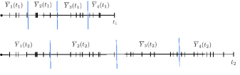
Figure 2: A sketch of the batch-means stopping rule. The process is simulated for a fixed number of jumps ($N_{J}=20$) to a terminal time $t_{1}$, and then the trajectory is partitioned into $N_{b}=4$ batches to compute the variance between the batch means $\overline{Y}_{k}(t_{1})$. If the confidence bounds are precise enough ($MOE(t_{1})\leq\delta_{precise}$), then the simulation is terminated and each batch gives an iid sample of $\mathcal{N}\left(f_{\pi},\sigma^{2}\right)$. Otherwise, another $N_{J}=20$ jumps are simulated and the process is repeated.

In addition to giving an on-line estimate of the relaxation time of the system, the Batch-Means Stopping Rule gives $N_{b}-1$ (nearly) independent samples of trajectories with initial distribution approximately equal to the stationary distribution. Furthermore, one can compute the reweighting coefficients $W_{k,\theta}(t)$ in each batch to give $N_{b}$ (nearly) independent samples of the steady-state reweighting coefficients (in a manner similar to the “Time-Averaged Correlation Function” method of Ref. (23)).

IV.2 Batch-Means Stopping Implementation

Suppose we have a general reaction network with $M_{r}$ reactions and $M_{\theta}$ reaction parameters. Here we allow the possibility that $M_{r}\neq M_{\theta}$ for general propensity functions $\lambda_{r}(x;{\boldsymbol{\theta}})$ (e.g. Michaelis-Menten kinetics), whose parameter derivatives $\partial_{\theta_{i}}\lambda_{r}(x;{\boldsymbol{\theta}})$ we can compute explicitly for all $i=1,\dots,M_{\theta}$ and all $r=1,\dots,M_{r}$. Denote by $\zeta_{r}$ the stoichiometric vector for the $r$th reaction. Our goal is to estimate the gradient $\nabla_{\theta}\mathbb{E}_{\pi({\boldsymbol{\theta}})}\left\{f(X)\right\}$ for some observable function $f$.

We introduce the following notation for the batch-means stopping rule. $\hat{X}(n)$ is the $n$th state of the reaction network, $T(n)$ is the time of the $n$th jump and $\hat{f}(n)=f(\hat{X}(n))$ for the value of the observable at the $n$th state. $F(n)=\int_{0}^{T(n)}f\left(X(s)\right)ds$ is the time-integrated value of $f$ up to the $n$th jump, $r^{*}(n)$ is the reaction which fires at jump $n$ (taking the system from $\hat{X}(n)$ to $\hat{X}(n+1)$), $\hat{e}_{i}$ is the vector in $\mathbb{R}^{1\times M_{\theta}}$ with $1$ in the $i$th component and zeros elsewhere. $R(n,{\boldsymbol{\theta}})\in\mathbb{R}^{1\times M_{\theta}}$ and $B(n,{\boldsymbol{\theta}})\in\mathbb{R}^{1\times M_{\theta}}$ are the first and second terms of (13) with respect to each of the parameters $\theta_{i}\in{\boldsymbol{\theta}}$ ($i=1,\dots,M_{\theta}$). $N_{b}$ is the number of batches (approximately independent samples) to be used, $\delta_{CI}$ is the desired confidence level (for a $(1-\delta_{CI})100\%$ confidence interval, and $\delta_{precise}$ is the maximum allowed radius of the confidence interval at the stopping time. $N_{J}$ is the number of jumps to simulate before retesting the batches for convergence. Then one can write the batch-means stopping rule as follows.

Algorithm 2 (Batch-Means Stopping Rule with Sensitivity Estimation).

1. Initialize

   • $\hat{X}(0)=x_{0}$, $\hat{f}(0)=f\left(\hat{X}(0)\right)$, $T(0)=0$, $F(0)=0$, $R(0)=[0,\dots,0]\in\mathbb{R}^{1\times M_{\theta}}$, $B(0)=[0,\dots,0]\in\mathbb{R}^{1\times M_{\theta}}$. ${tests}=0$ (number of times the data has been tested for convergence). Calculate $t_{quantile}=(1-\delta_{CI}/2)$ quantile of a Student’s $t$-distribution with $N_{b}-1$ degrees of freedom.

2. Generate and Record Data Simulate $N_{J}$ jumps and record values immediately after each jump. For $n=N_{J}\cdot{tests},\dots,N_{J}\cdot({tests}+1)-1$,

   • Compute $\lambda_{r}(\hat{X}(n);{\boldsymbol{\theta}})$, $\frac{\partial}{\partial\theta_{i}}\lambda_{r}(\hat{X}(n),{\boldsymbol{\theta}})$ for all $r=1,\dots,M_{r}$ and all $\theta_{i}=1,\dots M_{\theta}$. Set $\lambda_{0}(\hat{X}(n);{\boldsymbol{\theta}})=\sum_{r=1}^{M_{r}}\lambda_{r}(\hat{X}(n),{\boldsymbol{\theta}})$, and $\frac{\partial}{\partial\theta_{i}}\lambda_{0}(\hat{X}(n),{\boldsymbol{\theta}})=\sum_{r=1}^{M_{r}}\frac{\partial}{\partial\theta_{i}}\lambda_{r}(\hat{X}(n),{\boldsymbol{\theta}})$ for all $\theta_{i}\in{\boldsymbol{\theta}}$.

   • Sample $\Delta t(n)\sim\mathcal{E}{{xp}}\left(\lambda_{0}(\hat{X}(n),{\boldsymbol{\theta}})\right)$, and $r^{*}(n)\sim\frac{1}{\lambda_{0}(\hat{X}(n),{\boldsymbol{\theta}})}$
       $\qquad\times\left[\lambda_{1}(\hat{X}(n);{\boldsymbol{\theta}}),\dots,\lambda_{M_{r}}(\hat{X}(n);{\boldsymbol{\theta}})\right]$.

   • Update $T(n+1)=T(n)+\Delta t(n)$
     $\hat{X}(n+1)=\hat{X}(n)+\zeta_{r^{*}(n)}$
     $\hat{f}(n+1)=f(\hat{X}(n+1))$
     $F(n+1)=F(n)+\hat{f}(n)\cdot\Delta t(n)$
     $R(n+1,{\boldsymbol{\theta}})=R(n,{\boldsymbol{\theta}})+\sum_{i=1}^{M_{\theta}}\hat{e}_{i}\\ \qquad\times\ \left[\frac{\partial}{\partial\theta_{i}}\lambda_{r^{*}(n)}\left(\hat{X}(n),{\boldsymbol{\theta}}\right)\right]/\lambda_{r^{*}(n)}\left(\hat{X}(n),{\boldsymbol{\theta}}\right)$
     $\hat{b}(n,{\boldsymbol{\theta}})=\sum_{i=1}^{M_{\theta}}\hat{e}_{i}\cdot\left[\sum_{r=1}^{M_{r}}\frac{\partial}{\partial\theta_{i}}\lambda_{r}(\hat{X}(n),{\boldsymbol{\theta}})\right]$
     $B(n+1,{\boldsymbol{\theta}})=B(n,{\boldsymbol{\theta}})+\hat{b}(n,{\boldsymbol{\theta}})\cdot\Delta t(n)$
     $W(n+1,{\boldsymbol{\theta}})=R(n+1,{\boldsymbol{\theta}})-B(n+1,{\boldsymbol{\theta}})$.

3. Test Batches for Convergence

   • $N_{end}=N_{J}\cdot({tests}+1)$= index of last available data point.
     $\bar{Y}=F\left(N_{end}\right)/T(N_{end})$ = total time-averaged value
     $t_{batch}=T(N_{end})/N_{b}$= time length each of batch
     Initialize $F^{B}=0$ (total integral through end of previous batch).

   • for $k=1,\dots,N_{b}$

     • $ind_{B}(k)$= $\max\left\{n:T(n)\leq k\cdot t_{batch}\right\}$=index of the last jump in batch $k$.

     • $F_{A}^{B}(k)=F(ind_{B}(k))+\hat{f}(ind_{B}(k))$
       $\times\left[k\cdot t_{batch}-T(ind_{B}(k))\right]-F^{B}$=total integrated value of $f(X(s))$ inside batch $k$.

     • $\overline{Y}_{k}=F_{A}^{B}(k)/t_{batch}$= $k$th batch-mean

     • $F^{B}\leftarrow F^{B}+F_{A}^{B}(k)$ (update integral to end of previous batch)

   • $s_{N_{b}}^{2}=\frac{1}{N_{b}-1}\sum_{k=1}^{N_{b}}\left[\overline{Y}_{k}-\overline{Y}\right]^{2}$ = variance between batches

   • $MOE=t_{quantile}*\sqrt{s^{2}_{N_{b}}/N_{b}}$ = margin of error for confidence interval

   • If $MOE\leq\delta_{precise}$, then go to (4). Else, ${tests}\leftarrow{tests}+1$ and go back to (2).

4. Compute LR Weights in each batch.

   Initialize $W^{B}({\boldsymbol{\theta}})=[0,\dots,0]\in\mathbb{R}^{1\times M_{\theta}}$. For $k=1,\dots,N_{b}$,

   • $W_{A}^{B}(k,{\boldsymbol{\theta}})=W(ind_{B}(k),{\boldsymbol{\theta}})$
     $-\hat{b}(ind_{B}(k),{\boldsymbol{\theta}})\cdot\left[k\cdot t_{batch}-T(ind_{B}(k))\right]$
     $-W^{B}({\boldsymbol{\theta}})$

   • $W^{B}({\boldsymbol{\theta}})\leftarrow W^{B}({\boldsymbol{\theta}})+W_{A}^{B}(k,{\boldsymbol{\theta}})$

5. Compute Sensitivity Estimates for $\nabla_{\boldsymbol{\theta}}\mathbb{E}_{\pi({\boldsymbol{\theta}})}\left\{f(X)\right\}$:

   • Likelihood Ratio

     $${\bf LR}=\frac{1}{N_{b}}\sum_{k=1}^{N_{b}}\hat{f}\left(ind_{B}(k)\right)W_{A}^{B}(k,{\boldsymbol{\theta}})$$

   • Centered Likelihood Ratio

     $${\bf CLR}={\bf LR}\\ -\left[\frac{1}{N_{b}}\sum_{k=1}^{N_{b}}\hat{f}\left(ind_{B}(k)\right)\right]\cdot\left[\frac{1}{N_{b}}\sum_{k=1}^{N_{b}}W_{A}^{B}(k,{\boldsymbol{\theta}})\right]$$

   • Ergodic Likelihood Ratio

     $${\bf ELR}=\frac{1}{N_{b}}\sum_{k=1}^{N_{b}}\overline{Y}_{k}W_{A}^{B}(k,{\boldsymbol{\theta}})$$

   • Centered Ergodic Likelihood Ratio

     $${\bf CELR}={\bf ELR}-\left[\frac{1}{N_{b}}\sum_{k=1}^{N_{b}}\overline{Y}_{k}\right]\cdot\left[\frac{1}{N_{b}}\sum_{k=1}^{N_{b}}W_{A}^{B}(k,{\boldsymbol{\theta}})\right]$$

V Simulation Results

Here we present numerical results to display the performance of the proposed algorithms. In what follows, we compare the output of an exact simulation at the single time scale (STS) to the accelerated two time scale (TTS) approximation. From (11), we expect the differences in observable averages and their derivatives to be $O(\varepsilon)$. Because differences are small, we use a simple test system for which many samples can be run to obtain accurate statistics.

Consider a reaction network with species A, B, and C and isomerization reactions given by

$$\left.\begin{array}[]{rcl}A\overset{k_{1}/\varepsilon}{\rightarrow}B,&\quad B\overset{k_{2}/\varepsilon}{\rightarrow}A,&\quad B\overset{k_{3}}{\rightarrow}C\end{array}\right.$$

For small values of $\varepsilon$, the system becomes stiff as the isomerization between A and B reaches equilibrium much faster than B is converted to C. A TTS approximation assumes that $A\rightarrow B$ and $B\rightarrow A$ are fast and equilibrated.

We first compare the output of the accelerated TTS simulation against the exact STS simulation for varying levels of stiffness $\varepsilon$. For our simulations, initial conditions of $(A_{0},B_{0},C_{0})=(100,0,0)$ and the parameters $(k_{1},k_{2},k_{3})=(1,1.5,2)$ are chosen. 10,000 replicate (independent) trajectories are run for various values of $\varepsilon$. Statistics are taken at a termination time of $t=0.5$s. Species averages are calculated as arithmetic averages over the independent trajectories while sensitivities are computed with the CLR method shown in (15). The error due to statistical averaging is estimated using t-test statistics for averages and a bootstrapping method for sensitivities. Sensitivities with respect to the “slow” parameter $k_{3}$ are displayed for each species. As discussed in previous worksnunez_steady_2015 , sensitivities with respect to parameters related to fast reactions encounter significant noise, and thus we omit them in order to clearly observe the difference between STS and TTS. Figure 3 shows the disparity between the STS and TTS systems for various values of $\varepsilon$. Errors are normalized by the TTS value such that $\mathrm{Error}=\frac{\mathrm{STS}-\mathrm{TTS}}{|\mathrm{TTS}|}$. Indeed, one observes the difference is proportional to $\varepsilon$, as expected from Corollary II.5 and (11).

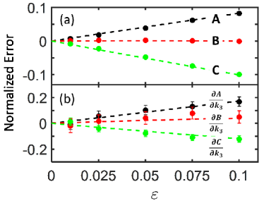
Figure 3: Normalized error of the two-time-scale (TTS) (accelerated, approximate) simulation from the exact single-time-scale (STS) simulation. The plot (a) shows errors in species averages while the plot (b) shows errors in sensitivities of each species with respect to $k_{3}$. Points indicate simulation statistics while dashed lines confirm the linear trend. The error bars are 95% confidence intervals of statistical noise.

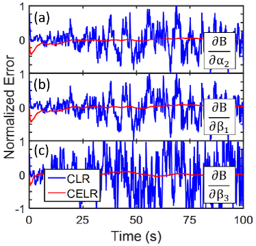
Figure 4: Time evolution of normalized errors obtained for sensitivities computed by CLR and CELR estimators. Simulation estimates are referenced and normalized by the analytical solution at each time point to compute the error. The graphs (a), (b), and (c) show estimates of different sensitivity indices for the species B. One observes that the variance of the CLR estimates increases with time, making for inefficient estimation. In contrast, the CELR estimates (the solid red line) converge quickly to the steady state sensitivities with variance which is roughly constant with time, allowing for efficient steady-state sensitivity estimation.

Next, the CLR and CELR methods from Section III.1 are tested in performing sensitivity analysis in a TTS system. The reaction network described in Section II.2 is simulated using Algorithm 1. To assess convergence of the microscale distribution, the batch-means stopping criterion described in Section IV is used with a tolerance of $\delta=0.05$. 1000 replicate trajectories are run to a time horizon of $t_{f}=100$s. The initial conditions used are $(A_{0},B_{0},*_{0})=(30,60,10)$ and the parameters used are $(\alpha^{\varepsilon}_{1},\alpha^{\varepsilon}_{2},\beta_{1},\beta_{2},\beta_{3})=(1/\varepsilon,1.5/\varepsilon,2,1,0.4)$.

Species populations, time-averaged species populations, and trajectory derivatives are recorded for each run over time. Using these recorded statistics, the sensitivities for all 15 (3 species and 5 parameters) species/parameter combinations are computed at each time point. Figure 4 shows the time evolution of the normalized errors in sensitivity estimates of the species B over time. Estimated values from simulation are referenced to the analytical answer as computed from a differential algebraic equation (see Appendix C) and normalized by that amount so that $\mathrm{Error}=\frac{\mathrm{estimated}-\mathrm{analytical}}{|\mathrm{analytical}|}$.

As expected, CLR estimates are noisy, with variance that grows linearly with time. At short times, the variance is small enough to obtain reasonable estimates. As time increases, the noise becomes significant with respect to the actual values (the magnitude of the normalized error becomes comparable to 1). In contrast, the ergodic likelihood ratio (CELR) fails at short times with a noticeable bias. However, the bias, which exists due to a relaxation period, decays as $O(1/t)$ when time increases and the system approaches its steady-state. The variance of the CELR estimates remain constant because the variance of trajectory derivatives increases linearly in time while the variance of ergodic species averages is proportional to $1/t$. At long times (where the CLR is too noisy for efficient estimation), the ergodic likelihood ratio obtains accurate estimates with very low variance. Therefore, it is advisable to use the CLR method for short times (in the transient regime) and the CELR method for long times to obtain steady state values.

Table 1 shows the error and statistical noise of the CLR and CELR estimations of sensitivities of the species B at a short ($t=1.3$s) and long ($t=100$s) times. Statistical noise is obtained from bootstrapping the samples used to compute the sensitivity estimates. At $t=1.3$, the CLR method has low error (theoretically, there is no bias) as well as low variance. The CELR estimator has a similarly low variance, but high error (due to the $O(1/t)$ bias). At $t=100$s, the CLR estimates have much higher variance which induces large empirical error. In contrast, the bias of the CELR estimate decreases in time while the variance remains low, providing very small empirical errors at large times.

Table 1: Comparison of the error and statistical noise for the CLR and CELR estimators at a short time (during the transient regime) and at a long time (corresponding to steady state). Values in the table refer to the sensitivity of the species B with respect to the parameter given by the row label. Values are reported as a percent of the analytically obtained sensitivity value.

	Percent Error
	CLR	CELR	CLR	CELR
	$t=1.3$s		$t=100$s
$\alpha_{1}$	-1.4	-40.0	-83.5	0.0
$\alpha_{2}$	-3.0	-40.3	-63.0	-1.1
$\beta_{1}$	0.2	-39.1	-64.1	1.2
$\beta_{2}$	-1.1	-16.7	-22.6	-2.8
$\beta_{3}$	-1.4	-23.3	20.6	-0.1
	Half-length of 95%
	Confidence Interval
$\alpha_{1}$	12	8	99	11
$\alpha_{2}$	12	7	94	11
$\beta_{1}$	12	7	91	11
$\beta_{2}$	13	10	108	12
$\beta_{3}$	21	14	171	18

VI Conclusions

This work develops a Two-Time-Scale (TTS) framework for multiscale reaction networks. By decomposing the system into “fast-classes”, one can approximate the behavior of the multiscale system by a lower-dimensional, single-scale, “macro-averaged” reaction network. By applying a singular perturbation expansion of the underlying probability measures, we have established rigorous bounds on the bias induced by the approximate macro-averaged model. We then proposed a TTS algorithm for simulating the macro reaction network, using an adaptive batch-means stopping rule for determining when the micro-scale dynamics have sufficiently equilibriated.

In addition, we have shown that the sensitivities of the macro-averaged system provide accurate approximations for the multiscale system. Since the macro-averaged system is single-scale, it is possible to incorporate most existing sensitivity estimation methods to the TTS algorithm to obtain estimates of the system sensitivities. We proposed an Ergodic Likelihood Ratio estimator for steady-state sensitivity analysis, and demonstrated how it can be adapted to the Two-Time-Scale algorithm. A simulation was then used to confirm the analytic error bounds and demonstrate the efficiency of the TTS Ergodic Likelihood Ratio estimator.

VII Acknowledgements

This work is supported by the U.S. Department of Energy Office of Science, Office of Advanced Scientific Computing Research, and Applied Mathematics program under Award No. DE-SC0010549.

Appendix A Analytic Stationary Sensitivities

For ergodic systems whose state space is relatively small (such that the generator $Q({\boldsymbol{\theta}})$ can be explicitly constructed), one can compute the steady-state probability vector $\pi({\boldsymbol{\theta}})$ by solving the linear system $\pi\cdot Q=\boldsymbol{0}$ and $\pi\cdot\boldsymbol{1}=1$. Here, we show that one can express the sensitivities of the steady-state measure $\frac{\partial}{\partial\theta}\pi({\boldsymbol{\theta}})$ explicitly as a linear transformation of the nominal measure $\pi({\boldsymbol{\theta}})$. The representation we shall construct is an adaptation of the discrete-time technique in Ref. (44) to continuous-time Markov chains, and exploits the algebraic properties of the pseudo-inverse $Q^{+}$ of $Q$.

By differentiating $\pi({\boldsymbol{\theta}})\cdot Q({\boldsymbol{\theta}})=\boldsymbol{0}$, we have the relation

$$\frac{\partial\pi}{\partial\theta}Q=-\pi\frac{\partial Q}{\partial\theta}$$

Then by expanding with the Moore-Penrose pseudo-inverse, we have

$$\left(\frac{\partial\pi}{\partial\theta}\right)^{\prime}=\left(Q\right)^{\prime}\left(\frac{-\partial Q}{\partial\theta}\right)^{\prime}\pi^{\prime}+\left[I-\left(Q^{\prime}\right)^{+}Q^{\prime}\right]w$$

for some vector $w$.

Now, we see by the projection property of $(Q^{\prime})^{+}Q^{\prime}=(QQ^{+})^{\prime}=QQ^{+}$ that the operator $I-QQ^{+}$ is the projection operator onto the kernel of $Q^{\prime}$ = span of $\pi^{\prime}$, so that $(I-QQ^{+})w=\gamma\pi^{\prime}$ for some scalar $\gamma$. Thus we have the relation

$$\frac{\partial\pi}{\partial\theta}=\pi\left(\frac{-\partial Q}{\partial\theta}\right)Q^{+}+\gamma\pi$$

for some $\gamma\in\mathbb{R}$. It remains to determine $\gamma$ to have a method of relating the sensitivity coefficient to a linear transformation of $\pi$.

Now, we can see that $\pi(\theta)\cdot\boldsymbol{1}=1$, so that $\frac{\partial\pi}{\partial\theta}\cdot\boldsymbol{1}=0$. Thus, we have

$$0=\frac{\partial\pi}{\partial\theta}\cdot\boldsymbol{1}=\pi\left(\frac{-\partial Q}{\partial\theta}\right)Q^{+}\boldsymbol{1}+\gamma\pi\boldsymbol{1}$$

so that

$$\gamma=\gamma\pi\boldsymbol{1}=\pi\frac{\partial Q}{\partial\theta}Q^{+}\boldsymbol{1}.$$

Putting the above together, we can write $\frac{\partial\pi}{\partial\theta}$ as

$$\frac{\partial\pi}{\partial\theta}=\pi\left(\frac{\partial Q}{\partial\theta}\right)Q^{+}\left[\boldsymbol{1}\pi-I\right].$$ (23)

For reaction networks with relatively small state space $\mathcal{M}$, (23) can provide a tractable method of computing the sensitivities of the steady-state measure $\frac{\partial\pi}{\partial\theta}$ and thus of the steady-state expected value

$$\frac{\partial}{\partial\theta}\mathbb{E}_{\pi({\boldsymbol{\theta}})}\left\{f(X;{\boldsymbol{\theta}})\right\}\\ =\sum_{x\in\mathcal{M}}\frac{\partial f(x;{\boldsymbol{\theta}})}{\partial\theta}\pi(x;{\boldsymbol{\theta}})+\sum_{x\in\mathcal{M}}f(x;{\boldsymbol{\theta}})\frac{\partial\pi(x;{\boldsymbol{\theta}})}{\partial\theta}.$$ (24)

For example, for reaction networks with mass-action propensities, the entries of $Q$ shall always be linear in the parameters $\theta$. Therefore, the derivatives $\frac{\partial Q}{\partial\theta}$ are easy to compute (whereas the stationary distribution $\pi({\boldsymbol{\theta}})$ can be quite complex as a function of $\theta$). Thus by computing the pseudo-inverse $Q^{+}$ from $Q$ at the nominal value of ${\boldsymbol{\theta}}$ (e.g., via singular value decomposition), one can analytically compute the system sensitivities without need of Monte Carlo simulation. For larger reaction networks, it may be possible to combine the Finite State Projection methodmunsky_finite_2006 ; sunkara_optimal_2010 with this pseudo-inverse technique to estimate the exact sensitivities by computing the analytic sensitivities of the reduced system.

Lastly, we use this representation to show that (21) holds. Write the exact generator $Q^{\varepsilon}$ as $Q^{\varepsilon}=Q({\boldsymbol{\theta}}^{\varepsilon})=(1/\varepsilon)\widetilde{Q}({{\boldsymbol{\alpha}}})+\widehat{Q}({{\boldsymbol{\beta}}})=\widetilde{Q}({{\boldsymbol{\alpha}}}^{\varepsilon})+\widehat{Q}({{\boldsymbol{\beta}}})$. For a fast reaction parameter $\alpha^{\varepsilon}_{i}=\alpha_{i}/\varepsilon$ a chain rule gives ${\partial_{\alpha_{i}}}\lambda(x;{{\boldsymbol{\alpha}}}^{\varepsilon})=\left[{\partial_{\alpha^{\varepsilon}_{i}}}\lambda(x;{{\boldsymbol{\alpha}}}^{\varepsilon})\right]/\varepsilon$, from which it follows (using (3)) that $\varepsilon\left[{\partial\alpha_{i}}\ \widetilde{Q}({{\boldsymbol{\alpha}}}^{\varepsilon})\right]={\partial_{\alpha_{i}}}\widetilde{Q}({{\boldsymbol{\alpha}}})={\partial_{\alpha^{\varepsilon}_{i}}}\widetilde{Q}({{\boldsymbol{\alpha}}}^{\varepsilon})$. Putting this relation into (23), we then have

$$\frac{\partial}{\partial\alpha^{\varepsilon}_{i}}\pi^{\varepsilon}=\varepsilon\left[\frac{\partial}{\partial\alpha_{i}}\pi^{\varepsilon}\right].$$ (25)

Similarly we see that $\partial\alpha_{i}\ f(x,{{\boldsymbol{\alpha}}}^{\varepsilon})=\left[\partial_{\alpha^{\varepsilon}_{i}}\ f(x,{{\boldsymbol{\alpha}}}^{\varepsilon})\right]/\varepsilon$. Finally, putting these relations into (25) we obtain (21),

$$\frac{\partial}{\partial\alpha^{\varepsilon}_{i}}\mathbb{E}_{\pi^{\varepsilon}}\left\{f(X;{{\boldsymbol{\alpha}}}^{\varepsilon},{{\boldsymbol{\beta}}})\right\}=\varepsilon\frac{\partial}{\partial\alpha_{i}}\mathbb{E}_{\pi^{\varepsilon}}\left\{f(X;{{\boldsymbol{\alpha}}}^{\varepsilon},{{\boldsymbol{\beta}}})\right\}.$$

Appendix B Proofs of Results

In this section we outline the proofs on the error bounds of the averaged reaction network and convergence of the sensitivities. The error bounds in this work are largely direct applications of the results in Ref. (20) to the Two-Time-Scale reaction networks formulated here. We present an overview of the proofs for insight and completeness. Similarly, the sensitivity convergence result comes from Ref. (14); we shall only how to fit their result to the Two-Time-Scale framework.

B.1 Proof of Theorem II.4:

Using the formulation of the exact generator $Q^{\varepsilon}({\boldsymbol{\theta}})=(1/\varepsilon)\widetilde{Q}({{\boldsymbol{\alpha}}})+\widehat{Q}({{\boldsymbol{\beta}}})$, the error bound on the induced probability measures of the exact and averaged systems is a direct application of Theorem 4.29 of Ref. (20). We outline the main steps below.

Write $p^{\varepsilon}(t)\in\mathbb{R}^{1\times m}$ for the probability measure of the exact system at time $t$. From the Kolmogorov forward equation (a.k.a. Chemical Master Equation), we have

$$\frac{dp^{\varepsilon}(t)}{dt}=p^{\varepsilon}(t)\left[\frac{1}{\varepsilon}\widetilde{Q}({{\boldsymbol{\alpha}}})+\widehat{Q}({{\boldsymbol{\beta}}})\right].$$ (26)

Define the differential operator $\mathcal{L}^{\varepsilon}$ on functions with values in $\mathbb{R}^{1\times m}$ by $\mathcal{L}^{\varepsilon}f=\varepsilon\frac{df}{dt}-f(\widetilde{Q}+\varepsilon\widehat{Q})$. Then $\mathcal{L}^{\varepsilon}f=0$ if and only if $f$ solves the CME (26). The form of the differential equation (26) suggests the plausibility of a singular perturbation expansion of $p^{\varepsilon}(t)$ by

$$p^{\varepsilon}(t)=\sum_{i=0}^{\infty}\varepsilon^{i}\phi_{i}(t)+\sum_{i=0}^{\infty}\varepsilon^{i}\psi_{i}\left(\frac{t}{\varepsilon}\right)$$ (27)

Assuming for the moment that such a representation holds, we proceed to derive the form of the “regular” terms $\phi_{i}(t)$ and the “boundary layer” terms $\psi_{i}(t)$. Applying $\mathcal{L}^{\varepsilon}$ to (27) and equating terms of $\varepsilon$ leads to the recursive equations

$$\begin{aligned} \varepsilon^{0}:&\qquad\phi_{0}(t)\widetilde{Q}=0\\ \varepsilon^{1}:&\qquad\phi_{1}(t)\widetilde{Q}=\frac{d\phi_{0}(t)}{dt}-\phi_{0}(t)\widehat{Q}\\ \vdots&\\ \varepsilon^{i}:&\qquad\phi_{i}(t)\widetilde{Q}=\frac{d\phi_{i-1}(t)}{dt}-\phi_{i-1}(t)\widehat{Q}\end{aligned}$$ (28)

and similarly, using the “stretched-time” variable $\tau=t/\varepsilon$ one has equations for $\psi(\tau)$

$$\begin{aligned} \varepsilon^{0}:&\qquad\frac{d\psi_{0}(\tau)}{d\tau}=\psi_{0}(\tau)\widetilde{Q}\\ \varepsilon^{1}:&\qquad\frac{d\psi_{1}(\tau)}{d\tau}=\psi_{1}(\tau)\widetilde{Q}-\psi_{0}(\tau)\widehat{Q}\\ \vdots&\\ \varepsilon^{i}:&\qquad\frac{d\psi_{i}(\tau)}{d\tau}=\psi_{i}(\tau)\widetilde{Q}-\psi_{i-1}(\tau)\widehat{Q}.\end{aligned}$$ (29)

At $t=0$,

$$\sum_{i=0}^{\infty}\varepsilon^{i}\left(\phi_{i}(0)+\psi_{i}(0)\right)=p^{\varepsilon}(0),$$ (30)

so $\phi_{0}(0)+\psi_{0}(0)=p^{\varepsilon}(0)$ and $\phi_{i}(0)+\psi_{i}(0)=0$ for all $i\geq 1$. Since $p^{\varepsilon}(t)$ is a probability measure with $p^{\varepsilon}(t)\cdot\boldsymbol{1}=1$, by sending $\varepsilon\to 0$ in (27) it follows that

$$\phi_{0}(t)\cdot\boldsymbol{1}=1\quad\text{ and }\quad\phi_{i}(t)\cdot\boldsymbol{1}=0$$ (31)

for all $t\in[0,T]$ and all $i\geq 1$.

Turning to the leading regular term $\phi_{0}(t)$, we note that $\phi_{0}(t)\cdot\widetilde{Q}=0$ is not uniquely solvable because $\widetilde{Q}={\operatorname{diag}}[\widetilde{Q}^{(1)},\dots,\widetilde{Q}^{({N_{C}})}]$ has rank $m-{N_{C}}$ However, writing $\phi^{(k)}_{0}(t)$ for the sub-vector of $\phi_{0}(t)$ corresponding to fast-class $\mathcal{M}_{k}$, then we must have $\phi^{(k)}_{0}(t)\cdot\widetilde{Q}^{(k)}=0$ for all $k=1,\dots,{N_{C}}$. Since each $\widetilde{Q}^{(k)}$ is an irreducible generator, we then have $\phi^{(k)}_{0}(t)=\gamma^{(k)}(t)\widetilde{\pi}^{(k)}$ for some scalar multiplier $\gamma^{(k)}(t)$. It can be seen (Prop 4.24yin_continuous-time_2013 ) that $\gamma^{(k)}(t)=\overline{p}_{k}(t)$, where $\overline{p}(t)$ is the probability measure among fast-classes $\mathcal{M}_{1},\dots,\mathcal{M}_{N_{C}}$ induced by generator $\overline{Q}$ (as in (5)) and initial distribution $p^{\varepsilon}(0)\cdot\widetilde{\boldsymbol{1}}=\mathbb{P}\left\{X^{\varepsilon}(0)\in\mathcal{M}_{k}\right\}$. This in turn determines a unique solution for $\phi^{(k)}_{0}(t)$ and therefore $\phi_{0}(t)$. It follows that $\phi_{0}(t)$ is exactly the measure $p^{0}_{t}$ in Theorem II.4 induced by the TTS simulation procedure.

With $\phi_{0}(t)$ determined, (30) then gives the initial condition $\psi_{0}(0)=p^{\varepsilon}(0)-\phi_{0}(0)=p^{\varepsilon}(0)[I_{m}-\widetilde{\boldsymbol{1}}\widetilde{\pi}]$, from which one can solve (29) to obtain $\psi_{0}(\tau)=\psi_{0}(0)\cdot\exp\left\{\widetilde{Q}\tau\right\}$. It can be shown (Prop. 4.25yin_continuous-time_2013 ) that

$$\|\psi_{0}(\tau)\|\leq C\exp\left\{-\widetilde{\kappa}\tau\right\},$$ (32)

where $C$ depends on the Jordan-Form of $\widetilde{Q}$. Higher order terms can also be solved for recursively (Prop. 4.26yin_continuous-time_2013 ), and it can be shown (Prop. 4.28yin_continuous-time_2013 )

$$\sup_{0\leq t\leq T}\|\sum_{i=0}^{n}\varepsilon^{i}\phi_{i}(t)+\sum_{i=0}^{n}\varepsilon^{i}\psi_{i}(t/\varepsilon)-p^{\varepsilon}(t)\|=O(\varepsilon^{n+1}).$$ (33)

In particular, using the $0$th-order expansion we have

$$\|p_{T}^{0}-p^{\varepsilon}_{T}\|=\|\phi_{0}(T)-p^{\varepsilon}(T)\|\\ \leq\|\phi_{0}(T)+\psi_{0}(T/\varepsilon)-p^{\varepsilon}(T)\|+\|\psi_{0}(T/\varepsilon)\|\\ \leq\|O(\varepsilon)+O(\exp{-\widetilde{\kappa}T/\varepsilon})\|$$ (34)

∎

B.2 Proof of Corollary II.5

With the singular perturbation bound (33), Corollary II.5 follows immediately. Since the exact process $X^{\varepsilon}(t)$ is ergodic, there exists a time horizon $T^{\varepsilon}$ such that $\|p^{\varepsilon}(t)-\pi^{\varepsilon}\|\leq\varepsilon$ for $t\geq T^{\varepsilon}$. Similarly, by (32) there exists $\widetilde{T}$ such that $\|\psi_{0}(t)\|\leq\varepsilon$ for $t\geq\widetilde{T}$, and $\|\overline{p}(t)-\overline{\pi}\|\leq\varepsilon$ for $t\geq\overline{T}$, implying that $\|\phi_{0}(t)-\overline{\pi}\widetilde{\pi}\|=\|\overline{p}(t)\widetilde{\pi}-\overline{\pi}\widetilde{\pi}\|\leq\varepsilon$. Then taking $T\geq\max\{T^{\varepsilon},\widetilde{T},\bar{T}\}$ and applying (33) , we have

$$\|p^{\varepsilon}(t)-\overline{\pi}\widetilde{\pi}\|\leq\|p^{\varepsilon}(t)-\phi(t)-\psi(t/\varepsilon)\|\\ +\|\phi(t)-\overline{\pi}\widetilde{\pi}\|+\|\psi(t/\varepsilon)\|\leq O\left(\varepsilon+\exp\left\{-\widetilde{\kappa}t/\varepsilon\right\}\right)\\ \|\pi^{\varepsilon}-\overline{\pi}\widetilde{\pi}\|\leq\|\pi^{\varepsilon}-p^{\varepsilon}(T)\|+\|p^{\varepsilon}(T)-\overline{\pi}\widetilde{\pi}\|\leq O(\varepsilon)$$

and the corollary follows. ∎

B.3 Proof of Proposition II.3

This is a direct application of Theorem 5.27yin_continuous-time_2013 , and also follows from the error bound (33). First, one uses (34) to establish that

$$\lim_{t\to 0}\lim_{\varepsilon\to 0}\mathbb{E}\left[\overline{X^{\varepsilon}}(s+t)-\overline{X^{\varepsilon}}(s)\big{|}X^{\varepsilon}(s)=x^{(k)}_{j}\right]=0$$

and thus $\left\{\overline{X^{\varepsilon}}(\cdot)\right\}_{\varepsilon>0}$ is tight. Then one shows that the finite-dimensional distributions converge by taking arbitrary time points $0\leq t_{1}<\dots<t_{n}\leq T$ and apply the Chapman-Kolmogorov equations to see

$$\mathbb{P}\left\{\overline{X^{\varepsilon}}(t_{n})=\overline{y}_{n},\dots,\overline{X^{\varepsilon}}(t_{1})=\overline{y}_{1}\right\}\\ =\sum_{j_{1},\dots,j_{n}}\mathbb{P}\left\{\overline{X^{\varepsilon}}(t_{n})=x^{(\overline{y}_{n})}_{j_{n}}\big{|}\overline{X^{\varepsilon}}(t_{n-1})=x^{(\overline{y}_{n-1})}_{j_{n-1}}\right\}\times\dots{\\ }\times\mathbb{P}\left\{\overline{X^{\varepsilon}}(t_{2})=x^{(\overline{y}_{2})}_{j_{2}}\big{|}\overline{X^{\varepsilon}}(t_{1})=x^{(\overline{y}_{1})}_{j_{1}}\right\}\\ \times\mathbb{P}\left\{\overline{X^{\varepsilon}}(t_{1})=x^{(\overline{y}_{1})}_{j_{1}}\right\}.$$

Then applying the error bound (34) to each transition term to obtain

$$\mathbb{P}\left\{\overline{X^{\varepsilon}}(t_{l})=x^{(\overline{y}_{l})}_{j_{l}}\Big{|}\overline{X^{\varepsilon}}(t_{l-1})=x^{(\overline{y}_{l-1})}_{j_{l-1}}\right\}\\ \to\mathbb{P}\left\{\overline{X}(t_{l})=\overline{y}_{l}\Big{|}\overline{X}(t_{l-1})=\overline{y}_{l-1}\right\}$$

as $\varepsilon\to 0$, and thus the finite dimensional distributions converge.

∎

B.4 Proof of Proposition III.1

Proposition III.1 is simply the application of Theorem 3.2 of Ref. (14) to the TTS framework. The method and framework for separating time-scales in Ref. (14) is slightly different than the TTS framework used here, but it can be seen that the two are equivalent. Here, we briefly review the multiscale framework of Ref. (14) and show how one can translate between their “remainder spaces” and the TTS “fast-classes”.

B.4.1 Scaling Rates and Remainder Spaces

As in Refs.(13; 18), Ref.(14) considers reaction rates of the form $a^{N}_{k}(x,\theta)=N^{\rho_{k}}\lambda_{k}(x,\theta)$ which scale with the “system size” or “normalization parameter” $N\gg 0$, where $\rho_{k}$ is the scaling rate for the $k$-th reaction channel. For a given normalizing parameter $N$, the corresponding system is denoted by $X^{N}(t)$. One analyzes the system against a reference time scale $\gamma$ by $X^{N}_{\gamma}(t)=X^{N}(tN^{\gamma})$. For a given normalizing parameter $N_{0}\gg 0$, the corresponding system is denoted by $X^{N_{0}}(t)$. One analyzes the system against a reference time scale $\gamma$ by $X^{N}_{\gamma}(t)=X^{N}(tN^{\gamma})$.

The scaling rates $\rho_{k}$ determine the time scales at which the reaction channels fire. For a system with with a single level of stiffness, there are only two scaling rates, $\rho_{fast}>\rho_{slow}$, which partition the reaction channels as either fast or slow. Write $\Gamma_{1}=\{k:\rho_{k}=\rho_{fast}\}$ for the fast reaction index set, and similarly $\Gamma_{2}$ for the slow reaction index set.

Take $\mathbb{S}_{2}=\{v\in\mathbb{R}^{d}_{+}:\langle v,\zeta_{k}\rangle=0\text{ for all }k\in\Gamma_{1}\}$ so that $\langle X_{\gamma}^{N}(t),v\rangle$ is unchanged by fast reactions. Then take $\mathbb{L}_{2}=\text{span}(\mathbb{S}_{2})$ and $\Pi_{2}$ be the projection map from $\mathbb{R}^{d}$ to $\mathbb{L}_{2}$, so that $\Pi_{2}\zeta_{k}=\boldsymbol{0}$ for all $k\in\Gamma_{1}$.

Let $\mathbb{L}_{1}=\text{span}\{(I-\Pi_{2})x:x\in\mathcal{M}\}$, and for any $v\in\Pi_{2}\mathcal{M}$ let $\mathbb{H}_{v}=\{y\in\mathbb{L}_{1}:y=(I-\Pi_{2})x,\Pi_{2}x=v,x\in\mathcal{M}\}$, the set of remainders of elements in $\mathcal{M}$ which get projected to $v$. Then we can define an operator $\mathbb{C}^{v}$ by

$$\mathbb{C}^{v}f(z)=\sum_{k\in\Gamma_{1}}\lambda_{k}(v+z,\theta)[f(z+\zeta_{k})-f(z)]$$

which is a generator of a Markov chain with state space $\mathbb{H}_{v}$ (note that $y\in\mathbb{H}_{v}\implies y+\zeta_{k}\in\mathbb{H}_{v}$ for all $k\in\Gamma_{1}$).

Assuming $\mathbb{H}_{v}$ under $\mathbb{C}^{v}$ is ergodic, there is a stationary distribution $\pi^{v}$. Then for each slow reaction $k\in\Gamma_{2}$ one can define the “averaged” propensities $\hat{\lambda}_{k}(v,\theta)=\int_{\mathbb{H}_{v}}\lambda_{k}(v+z,\theta)\pi^{v}(dz)$ for all $v\in\Pi_{2}\mathcal{M}$ . Using the random time change representation, define the Markov chain on $\Pi_{2}\mathcal{M}$ by

$$\hat{X}_{\theta}(t)=\Pi_{2}x_{0}+\sum_{k\in\Gamma_{2}}Y_{k}\left(\int_{0}^{t}\hat{\lambda}_{k}(\hat{X}(s),\theta)ds\right)\Pi_{2}\zeta_{k}$$ (35)

Taking $\gamma_{2}=-\rho_{slow}$ as the slow time scale, one has $\Pi_{2}X^{N}_{\gamma_{2},\theta}\Rightarrow\hat{X}_{\theta}$ as $N\to\infty$kang_separation_2013 under more general conditions than Assumptions II.1,II.2. Under this context, Theorem 3.2 of Ref.(14) states that

$$\lim_{N\to\infty}\frac{\partial}{\partial\theta}\mathbb{E}\left\{f(X^{N}_{\gamma_{2},\theta}(t))\right\}=\frac{\partial}{\partial\theta}\mathbb{E}\left\{f_{\theta}(\hat{X}_{\theta}(t))\right\}$$ (36)

where $f_{\theta}(v)=\int_{\mathbb{H}_{v}}f(v+y)\pi^{v}_{\theta}(dy)$.

B.4.2 Equivalence of Fast-Classes and Remainder Spaces

Here we show how the TTS framework is equivalent to the scaling rate framework. Consider a TTS reaction network as described by (3). Taking $N=1/\varepsilon$, $\rho_{fast}=1$, $\rho_{slow}=0$, it is easy to see that

$$X^{N}_{0,\theta}(t)=X^{N}_{\theta}(t)\overset{\mathcal{D}}{=}X^{\varepsilon}(t).$$

so $\lim_{N\to\infty}X^{N}_{0,\theta}(t)=\lim_{\varepsilon\to 0}X^{\varepsilon}(t)$. It remains to identify $f_{\theta}\left(\hat{X}_{\theta}(t)\right)$ from (35), (36) with $\overline{f}\left(\overline{X}(t)\right)$ from (8). We do so by showing the equivalence of the fast-classes $\mathcal{M}_{l}$ and the remainder spaces $\mathbb{H}_{v}$.

Lemma B.1.

The projection map $\Pi_{2}$ is invariant on fast-classes $\mathcal{M}_{l}$. The set of remainder spaces $\left\{\mathbb{H}_{v}:v\in\Pi_{2}\mathcal{M}\right\}$ is in one-to-one correspondence with the set of fast-classes $\left\{\mathcal{M}_{l}\right\}$. Additionally, each $x\in\mathcal{M}_{l}$ corresponds to a unique element $y\in\mathbb{H}_{v}$ for some $v\in\Pi_{2}\mathcal{M}$.

Proof.

Define $\eta:\left\{\mathcal{M}_{l}\right\}\to\left\{\mathbb{H}_{v}:v\in\Pi_{2}\mathcal{M}\right\}$ by

$$\eta(\mathcal{M}_{l})=\mathbb{H}_{\Pi_{2}(x)}\qquad\text{for any }x\in\mathcal{M}_{l}.$$

Then $\eta$ is well-defined, since $x,y\in\mathcal{M}_{l}$ implies that $y=x+\sum_{k\in\Gamma_{1}}c_{k}\zeta_{k}$ for some $c_{k}\in\mathbb{N}$, and $\Pi_{2}(\zeta_{k})=\boldsymbol{0}$ for all $k\in\Gamma_{1}$ gives $\Pi_{2}(y)=\Pi_{2}(x)$. Clearly, $\eta$ is also onto.

It remains to establish $\eta$ is injective. It is sufficient to show that if $\Pi_{2}(x)=v$ and $\Pi_{2}(x^{\prime})=v$ for $x,x^{\prime}\in\mathcal{M}$, then $x$ and $x^{\prime}$ belong to the same fast-class $\mathcal{M}_{l}$. Since $\Pi_{2}$ projects onto the span of the complement of $\operatorname{span}\left\{\zeta_{k}:k\in\Gamma_{1}\right\}$, we have $v-x=\sum_{k\in\Gamma_{1}}c_{k}\zeta_{k}$ and $v-x^{\prime}=\sum_{k\in\Gamma_{1}}c^{\prime}_{k}\zeta_{k}$ for some $c_{k},c^{\prime}_{k}\in\mathbb{R}$. Then $x^{\prime}=x+\sum_{k\in\Gamma_{1}}(c_{k}-c^{\prime}_{k})\zeta_{k}$, with $x^{\prime},x,\zeta_{k}\in\mathbb{N}^{d}$, so it follows that $(c_{k}-c^{\prime}_{k})\in\mathbb{N}$ for all $k$. Hence $x$ and $x^{\prime}$ communicate by fast reactions and thus belong to the same fast-class $\mathcal{M}_{l}$. Therefore, $\Pi_{2}$ is invariant on fast-classes and $\eta$ is injective.

Finally, since $\Pi_{2}(\cdot)$ is invariant on fast-classes $\mathcal{M}_{l}$, it follows that $x\to x-\Pi_{2}(x)$ bijectively maps elements of $\cup_{l}\mathcal{M}_{l}$ to elements of $\cup_{v\in\Pi_{2}(\mathcal{M})}\mathbb{H}_{v}$ such that $x,x^{\prime}\in\mathcal{M}_{l}$ implies $(x-\Pi_{2}(x)),(x^{\prime}-\Pi_{2}(x^{\prime}))\in\mathbb{H}_{\Pi_{2}(\mathcal{M}_{l})}$. ∎

Because of the direct correspondence between $\left\{\Pi_{2}(x):x\in\mathcal{M}\right\}$ and $\left\{\mathcal{M}_{l}\right\}$, we see (upon reordering states) that for $v=\Pi_{2}(\mathcal{M}_{l})$, we have $\pi^{v}_{\theta}=\widetilde{\pi}^{(l)}_{\theta}$, so that $\hat{\lambda}_{k}(v,\theta)=\overline{\lambda}_{k}(\mathcal{M}_{l},\theta)$, and $f_{\theta}(v)=\overline{f}(\mathcal{M}_{l},\theta)$. Thus, $f_{\theta}\left(\hat{X}(t)\right)$ has the same distribution as $\overline{f}\left(\mathcal{M}_{l},\theta\right)$ and so $\frac{\partial}{\partial\theta}\mathbb{E}\left\{f_{\theta}\left(\hat{X}_{\theta}(t)\right)\right\}=\frac{\partial}{\partial\theta}\mathbb{E}\left\{\overline{f}\left(\overline{X}_{\theta}(t)\right)\right\}$. Therefore, using (36) we have

$$\begin{aligned} \lim_{\varepsilon\to 0}\partial_{\theta}\mathbb{E}\left\{f\left(X^{\varepsilon}(t)\right)\right\}=\lim_{N\to\infty}\partial_{\theta}\mathbb{E}\left\{f\left(X^{N}_{0,\theta}(t)\right)\right\}\\ =\partial_{\theta}\mathbb{E}\left\{f_{\theta}\left(\hat{X}_{\theta}(t)\right)\right\}=\partial_{\theta}\mathbb{E}\left\{\overline{f}\left(\overline{X}(t)\right)\right\}\end{aligned}$$ (37)

and hence Proposition III.1.

Appendix C Analytic solution of the Model System

In a well-mixed system with linear propensities, the time-evolution of the system can be obtained from a set of ordinary differential equations (ODE). The single time-scale (STS) system can be modeled with a system of ODEs. The two time-scale (TTS) system imposes algebraic constraints for the fast modes, resulting in an algebraic differential system of equations. In both cases, a set of adjoint ODEs can be used to compute sensitivities alongside species populations.

In our model system, gaseous species A adsorbs onto a catalyst surface, isomerizes to species B, and then desorbs. A diagram of the reaction network is shown in Figure 5. The reactions along with their rate laws are shown in Table 5. $N_{A}$, $N_{B}$, and $N_{*}$ denote the surface coverages of species A, B, and empty sites respectively. The adsorption/desorption of species A is assumed to be much faster than the others. The separation of time scales is captured with the dimensionless parameter $\varepsilon<<1$. The system contains $M=3$ species and $R=6$ reactions. Mathematically, we use the $M\times 1$ column vector $N$ to specify the species populations, where $N_{1}=N_{A}$, $N_{2}=N_{B}$, and $N_{3}=N_{*}$.

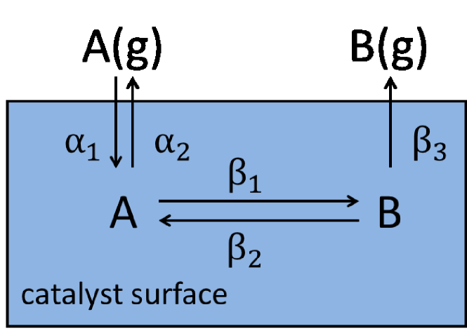
(a) Visual diagram of reaction network.

Index	Reaction	Rate
1	$*\rightarrow A$	$\varepsilon^{-1}\alpha_{1}N_{*}$
2	$A\rightarrow*$	$\varepsilon^{-1}\alpha_{2}N_{A}$
3	$A\rightarrow B$	$\beta_{1}N_{A}$
4	$B\rightarrow A$	$\beta_{2}N_{B}$
5	$B\rightarrow*$	$\beta_{3}N_{B}$

(b) Reactions for the benchmark network.

Figure 5: Description of model chemical reaction network.

The linear dependence of the reaction rates is written as

$$r(N)=\left[\begin{array}[]{c}\varepsilon^{-1}\alpha_{1}N_{3}\\ \varepsilon^{-1}\alpha_{2}N_{1}\\ \beta_{1}N_{1}\\ \beta_{2}N_{2}\\ \beta_{3}N_{2}\end{array}\right].$$ (38)

Each row of the stoichiometric matrix corresponds to a different species, which are $N_{1}$, $N_{2}$, and $N_{3}$ respectively. The columns correspond to each of reactions 1-5 in order. Extracting the information from Table 5 and putting it in mathematical form gives the $M\times R$ stoichiometric matrix

$$S=\left[\begin{array}[]{ccccc}1&-1&-1&1&0\\ 0&0&1&-1&1\\ -1&1&0&0&-1\end{array}\right]$$ (39)

The transformation matrix

$$T=\left[\begin{array}[]{ccc}1&0&0\\ 0&1&0\\ 1&1&1\end{array}\right].$$ (40)

yields $y=T\cdot N$ and $T$ can be decomposed into $T_{f}=\left[\begin{array}[]{ccc}1&0&0\end{array}\right]$ and $T_{s}=\left[\begin{array}[]{ccc}1&1&0\\ 0&0&1\end{array}\right]$ for the slow modes by looking at the 0 rows of $S^{\prime}_{f}$. This gives us the transformed variables as $y_{f}=\left[\begin{array}[]{c}N_{1}\end{array}\right]$ and $y_{s}=\left[\begin{array}[]{c}N_{2}\\ N_{1}+N_{2}+N_{3}\end{array}\right]$.

In the context of our example problem, we can assign physical meaning to the transformation: The variable $y_{1}=N_{A}$ is affected by both slow and fast reactions. For a given set of slow variables, we can solve for $y_{1}$ to specify the equilibrium constraint of $r_{1}=r_{2}$. The variable $y_{2}=N_{B}$ is unaffected by the fast adsorption/desorption of A, but is affected by the slow reactions. Finally, the variable $y_{3}=N_{A}+N_{B}+N_{*}$ is a second ”slow” variable. In this example $y_{3}=1$ applies at all times due to stoichiometric constraints. However, it is still identified as a ”slow mode” because this constraint is not a consequence of disparities in reaction time scales.

The system is simulated with the choice of parameters $N_{0}=\left[\begin{array}[]{c}30\\ 60\\ 10\end{array}\right]$, $\alpha_{1}=1$, $\alpha_{2}=1.5$, $\beta_{1}=2$, $\beta_{2}=1$, $\beta_{3}=0.4$, $\varepsilon=0.01$. The simulation results are shown in Figure 6. Table 2 shows values at $t=1.3$s and $t=100$s along with CLR and CELR estimates with statistical confidence intervals. Derivatives with respect to $\beta_{2}$ and $\beta_{3}$ overlap because both affect system properties through the the independent parameter $\beta_{2}+\beta_{3}$.

In general, the system parameters need not be the rate constants themselves. A different parameterization would involve a transformation of the rate constants. Sensitivities could be obtained through a chain rule.

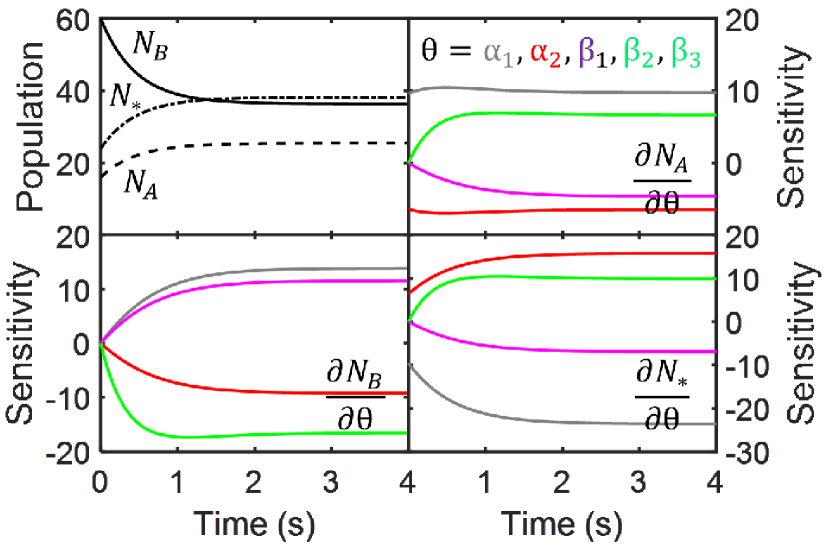
Figure 6: Network results for the two time-scale system. Graphs show population counts (top left), derivatives of species A (top right), derivatives of species B (bottom left), and derivatives of empty sites (bottom right).

Table 2: Comparison of the CLR and CELR estimators with the ODE solution. Values show actual values rather than errors. Values in the table refer to the sensitivity of the species B with respect to the parameter given by the row label. 95% confidence intervals are based on statistical noise.

	$t=1.3$s
	ODE	CLR	CELR
$\alpha_{1}$	11.9	$11.8\pm 1.5$	$7.2\pm 0.9$
$\alpha_{2}$	-7.9	$-7.7\pm 1.0$	$-4.7\pm 0.6$
$\beta_{1}$	9.9	$10.0\pm 1.2$	$6.0\pm 0.8$
$\beta_{2}$	-17.4	$-17.2\pm 2.4$	$-14.5\pm 1.7$
$\beta_{3}$	-17.4	$-17.1\pm 3.4$	$-13.3\pm 2.4$
	$t=100$s
	ODE	CLR	CELR
$\alpha_{1}$	13.9	$2.3\pm 13.7$	$13.9\pm 1.4$
$\alpha_{2}$	-9.3	$-3.4\pm 8.9$	$-9.2\pm 1.0$
$\beta_{1}$	11.6	$4.1\pm 10.6$	$11.7\pm 1.2$
$\beta_{2}$	-16.5	$-12.8\pm 18.1$	$-16.1\pm 2.0$
$\beta_{3}$	-16.5	$-19.9\pm 29.0$	$-16.5\pm 3.2$

References

- (1) Abhijit Chatterjee and Dionisios G Vlachos. An overview of spatial microscopic and accelerated kinetic Monte Carlo methods. Journal of Computer-Aided Materials Design, 14(2):253–308, 2007.
- (2) Daniel T. Gillespie. Approximate accelerated stochastic simulation of chemically reacting systems. The Journal of Chemical Physics, 115(4):1716–1733, July 2001.
- (3) Yang Cao, Daniel T. Gillespie, and Linda R. Petzold. Avoiding negative populations in explicit Poisson tau-leaping. The Journal of Chemical Physics, 123(5):054104, August 2005.
- (4) Yang Cao, Daniel T. Gillespie, and Linda R. Petzold. Efficient step size selection for the tau-leaping simulation method. The Journal of Chemical Physics, 124(4):044109, January 2006.
- (5) Muruhan Rathinam, Linda R. Petzold, Yang Cao, and Daniel T. Gillespie. Stiffness in stochastic chemically reacting systems: The implicit tau-leaping method. The Journal of Chemical Physics, 119(24):12784–12794, December 2003.
- (6) Abhijit Chatterjee, Dionisios G. Vlachos, and Markos A. Katsoulakis. Binomial distribution based τ-leap accelerated stochastic simulation. The Journal of Chemical Physics, 122(2):024112, January 2005.
- (7) Tianhai Tian and Kevin Burrage. Binomial leap methods for simulating stochastic chemical kinetics. The Journal of Chemical Physics, 121(21):10356–10364, December 2004.
- (8) Howard Salis and Yiannis Kaznessis. Accurate hybrid stochastic simulation of a system of coupled chemical or biochemical reactions. The Journal of Chemical Physics, 122(5):054103, February 2005.
- (9) A. Samant and D. G. Vlachos. Overcoming stiffness in stochastic simulation stemming from partial equilibrium: A multiscale Monte Carlo algorithm. The Journal of Chemical Physics, 123(14):144114, October 2005.
- (10) Yang Cao, Daniel T. Gillespie, and Linda R. Petzold. The slow-scale stochastic simulation algorithm. The Journal of Chemical Physics, 122(1):014116, January 2005.
- (11) Weinan E, Di Liu, and Eric Vanden-Eijnden. Nested stochastic simulation algorithms for chemical kinetic systems with multiple time scales. Journal of Computational Physics, 221(1):158–180, January 2007.
- (12) Can Huang and Di Liu. Strong convergence and speed up of nested stochastic simulation algorithm. Commun. Comput. Phys, 15:1207–1236, 2014.
- (13) Hye-Won Kang and Thomas G. Kurtz. Separation of time-scales and model reduction for stochastic reaction networks. The Annals of Applied Probability, 23(2):529–583, April 2013.
- (14) Ankit Gupta and Mustafa Khammash. Sensitivity analysis for stochastic chemical reaction networks with multiple time-scales. Electron. J. Probab, 19(59):1–53, 2014.
- (15) Paul Dupuis, Markos A. Katsoulakis, Yannis Pantazis, and Petr Plechac. Path-space information bounds for uncertainty quantification and sensitivity analysis of stochastic dynamics. arXiv:1503.05136 [math], March 2015. arXiv: 1503.05136.
- (16) Elizabeth Skubak Wolf and David F. Anderson. Hybrid pathwise sensitivity methods for discrete stochastic models of chemical reaction systems. The Journal of Chemical Physics, 142(3):034103, January 2015.
- (17) Patrick W. Sheppard, Muruhan Rathinam, and Mustafa Khammash. A pathwise derivative approach to the computation of parameter sensitivities in discrete stochastic chemical systems. The Journal of Chemical Physics, 136(3):034115, January 2012.
- (18) Ting Wang and Muruhan Rathinam. Efficiency of the Girsanov transformation approach for parametric sensitivity analysis of stochastic chemical kinetics. arXiv:1412.1005 [math], December 2014. arXiv: 1412.1005.
- (19) Ankit Gupta and Mustafa Khammash. An efficient and unbiased method for sensitivity analysis of stochastic reaction networks. arXiv:1402.3076 [math], February 2014. arXiv: 1402.3076.
- (20) George Yin and Qing Zhang. Continuous-Time Markov Chains and Applications: A Two-Time-Scale Approach. Springer, New York, 2013.
- (21) M. Núñez and D. G. Vlachos. Steady state likelihood ratio sensitivity analysis for stiff kinetic Monte Carlo simulations. The Journal of Chemical Physics, 142(4):044108, January 2015.
- (22) Sergey Plyasunov and Adam P. Arkin. Efficient stochastic sensitivity analysis of discrete event systems. Journal of Computational Physics, 221(2):724–738, February 2007.
- (23) Patrick B. Warren and Rosalind J. Allen. Steady-state parameter sensitivity in stochastic modeling via trajectory reweighting. arXiv:1202.4704 [physics, q-bio], February 2012. arXiv: 1202.4704.
- (24) P. W. Glynn. Likelihood ratio gradient estimation for stochastic systems. Communications of the ACM, 33(10):75–84, 1990.
- (25) David F. Anderson and Thomas G. Kurtz. Continuous Time Markov Chain Models for Chemical Reaction Networks. In Heinz Koeppl, Gianluca Setti, Mario di Bernardo, and Douglas Densmore, editors, Design and Analysis of Biomolecular Circuits, pages 3–42. Springer New York, January 2011.
- (26) Stewart N. Ethier and Thomas G. Kurtz. Markov Processes: Characterization and Convergence. John Wiley & Sons, 1986.
- (27) Michael A. Gibson and Jehoshua Bruck. Efficient Exact Stochastic Simulation of Chemical Systems with Many Species and Many Channels. The Journal of Physical Chemistry A, 104(9):1876–1889, March 2000.
- (28) David F. Anderson. A modified next reaction method for simulating chemical systems with time dependent propensities and delays. The Journal of Chemical Physics, 127(21):214107, December 2007.
- (29) Muruhan Rathinam, Patrick W. Sheppard, and Mustafa Khammash. Efficient computation of parameter sensitivities of discrete stochastic chemical reaction networks. The Journal of Chemical Physics, 132(3):034103, January 2010.
- (30) D. Anderson. An Efficient Finite Difference Method for Parameter Sensitivities of Continuous Time Markov Chains. SIAM Journal on Numerical Analysis, 50(5):2237–2258, January 2012.
- (31) Ankit Gupta and Mustafa Khammash. Sensitivity analysis for stochastic chemical reaction networks with multiple time-scales. arXiv:1310.1729 [math], October 2013. arXiv: 1310.1729.
- (32) Yannis Pantazis, Markos A Katsoulakis, and Dionisios G Vlachos. Parametric sensitivity analysis for biochemical reaction networks based on pathwise information theory. BMC Bioinformatics, 14:311, October 2013.
- (33) Jacob A. McGill, Babatunde A. Ogunnaike, and Dionisios G. Vlachos. Efficient gradient estimation using finite differencing and likelihood ratios for kinetic Monte Carlo simulations. Journal of Computational Physics, 231(21):7170–7186, August 2012.
- (34) Søren Asmussen and Peter W. Glynn. Stochastic Simulation: Algorithms and Analysis. Springer Science & Business Media, July 2007.
- (35) Yang Cao, Dan Gillespie, and Linda Petzold. Multiscale stochastic simulation algorithm with stochastic partial equilibrium assumption for chemically reacting systems. Journal of Computational Physics, 206(2):395–411, July 2005.
- (36) David Asher Levin, Yuval Peres, and Elizabeth Lee Wilmer. Markov Chains and Mixing Times. American Mathematical Soc., 2009.
- (37) Charles J. Geyer. Practical Markov Chain Monte Carlo. Statistical Science, 7(4):473–483, November 1992.
- (38) C. Kipnis and S. R. S. Varadhan. Central limit theorem for additive functionals of reversible Markov processes and applications to simple exclusions. Communications in Mathematical Physics, 104(1):1–19, March 1986.
- (39) Bernd A. Berg. Introduction to Markov Chain Monte Carlo Simulations and their Statistical Analysis. arXiv:cond-mat/0410490, October 2004. arXiv: cond-mat/0410490.
- (40) A. Sokal. Monte Carlo methods in statistical mechanics: foundations and new algorithms. In Functional integration, pages 131–192. Springer, 1997.
- (41) Sean P. Meyn and Richard L. Tweedie. Markov Chains and Stochastic Stability. Cambridge University Press, April 2009.
- (42) Christos Alexopoulos and Andrew F. Seila. Implementing the Batch Means Method in Simulation Experiments. In Proceedings of the 28th Conference on Winter Simulation, WSC ’96, pages 214–221, Washington, DC, USA, 1996. IEEE Computer Society.
- (43) Peter W. Glynn and Donald L. Iglehart. Simulation Output Analysis Using Standardized Time Series. Mathematics of Operations Research, 15(1):1–16, February 1990.
- (44) R. E. Funderlic and C. D. Meyer Jr. Sensitivity of the stationary distribution vector for an ergodic Markov chain. Linear Algebra and its Applications, 76:1–17, April 1986.
- (45) Brian Munsky and Mustafa Khammash. The finite state projection algorithm for the solution of the chemical master equation. The Journal of Chemical Physics, 124(4):044104, January 2006.
- (46) Vikram Sunkara and Markus Hegland. An optimal Finite State Projection Method. Procedia Computer Science, 1(1):1579–1586, May 2010.