Gauged Nambu-Jona-Lasinio inflation

Tomohiro Inagaki1,2, Sergei D. Odintsov3,4,5, and Hiroki Sakamoto5,
1Information Media Center, Hiroshima University, Higashi-Hiroshima, 739-8521, Japan,
2Core of Research for the Energetic Universe, Hiroshima University, Higashi-Hiroshima,
739-8526, Japan,
3Institució Catalana de Recerca i Estudis Avançats (ICREA), Barcelona, Spain,
4Consejo Superior de Investigaciones Científicas, ICE/CSIC-IEEC, Campus UAB,
Torre C5-Parell-2a pl, E-08193 Bellaterra (Barcelona), Spain,
5Lab. Theor. Cosmology, Tomsk State University of Control Systems and Radioelectronics
(TUSUR), 634050 Tomsk, Russia,
5Department of Physics, Hiroshima University, Higashi-Hiroshima, 739-8526, Japan
Abstract

We investigate the gauged Nambu-Jona-Lasinio model in curved spacetime at the large Ncsubscript𝑁𝑐N_{c} limit and in slow-roll approximation. The model can be described by the renormalization group corrected gauge-Higgs-Yukawa theory with the corresponding compositeness conditions. Evaluating the renormalization group (RG) improved effective action, we show that such model can produce CMB fluctuations and find inflationary parameters: spectral index, tensor-to-scalar-ratio and running of the spectral index. We demonstrate that the model can naturally satisfy the Planck 2015 data and maybe considered as an alternative candidate for Higgs inflation.
Keyword: gauged Nambu-Jona-Lasinio model, CMB fluctuations
PACS: 04.62.+v 12.60.Rc 98.80.Cq

1 Introduction

The standard model of the particle physics is based on the gauge symmetry and the symmetry breaking. For example, QCD is described as SU(3)𝑆𝑈3SU(3) gauge theory. The gauge interaction causes chiral symmetry breaking. Because of the strong coupling constant, low energy phenomena are often approximated by using effective models. For instance, Nambu-Jona-Lasinio (NJL) model [1] is a well-known model for light mesons. Gauged NJL model maybe applied to the description of QCD, as SU(Nc)𝑆𝑈subscript𝑁𝑐SU(N_{c}) gauge theory, in which the chiral symmetry is broken and meson like composite fields are generated at high energy scale (see, for example [2]). The renormalizability of the model is precisely studied by using the ladder Schwinger-Dyson equation in flat spacetime [3]. In the leading order of the 1/Nc1subscript𝑁𝑐1/N_{c} expansion the model can be described by a gauge-Higgs-Yukawa type Lagrangian with compositeness conditions [4].

Gauged NJL model is expected to be very important at the early universe111Constraints from the high energy collider physics are reviewed in Ref. [5].. The vacuum energy for a fermion field is negative, unlike to the scalar field. After the dynamical symmetry breaking a composite scalar can develop a positive vacuum energy. A primordial potential energy for the composite scalar may induce inflation, i.e. exponential expansion of our universe. An evidence of inflation is observed in the cosmic microwave background radiation (CMB) [6, 7]. In this paper we propose gauged NJL inflation model as an alternative to Higgs inflation. We evaluate the CMB fluctuations in the gauged NJL model and demonstrate that inflationary parameters are consistent with Planck bounds.

The study of NJL model in curved space-time has been started some time ago (for review, see Ref. [8]). The curvature coupling for the composite scalar field has been obtained in Ref. [9, 10]. In the gauged NJL model it has been shown that the chiral symmetry can be broken for a strong curvature [11]. In Ref. [12] the authors have discussed the contributions from the dynamical symmetry breaking to the expansion of the universe. However, as far as we know there is only preliminary work to argue a contribution from composite fields to the CMB fluctuations. For instance, in Ref. [13] the authors have assumed non-vanishing fermion condensation and evaluated the CMB fluctuations.

This article is organized as follows: In Sec. 2 the gauged NJL model is introduced. The model is rewritten as renormalization-group corrected gauge-Higgs-Yukawa Lagrangian with compositeness conditions. In this way, this looks qualitatively similar to the study of RG improved effective potential in curved spacetime [14] and corresponding RG improved inflation [15]. In Sec. 3 we calculate the inflationary parameters in the gauged NJL model under the slow -roll approximation scenario. In Sec. 4 the inflationary parameters are numerically calculated and compared with the Planck data. Then we find a possible parameters range consistent with Planck data for the gauged NJL model. In Sec. 5 we briefly discuss an exit from inflation. Some concluding remarks are given in Sec. 6.

2 Gauged NJL model

We consider Nfsubscript𝑁𝑓N_{f} fermion flavors with SU(Nc)𝒢tensor-product𝑆𝑈subscript𝑁𝑐𝒢SU(N_{c})\otimes{\cal G} gauge symmetry. It is assumed that the gauge interaction for 𝒢𝒢\cal{G} is strong enough and well described by four-fermion interaction. We employ the gauged NJL model as an effective model of the SU(Nc)𝒢tensor-product𝑆𝑈subscript𝑁𝑐𝒢SU(N_{c})\otimes{\cal G} gauge theory. The Lagrangian is given by

gNJL=gauge+ψ¯i^ψ+16π2g48NfNcΛ2[(ψ¯ψ)2+(ψ¯iγ5τaψ)2],subscript𝑔𝑁𝐽𝐿subscript𝑔𝑎𝑢𝑔𝑒¯𝜓𝑖^italic-D̸𝜓16superscript𝜋2subscript𝑔48subscript𝑁𝑓subscript𝑁𝑐superscriptΛ2delimited-[]superscript¯𝜓𝜓2superscript¯𝜓𝑖subscript𝛾5superscript𝜏𝑎𝜓2\displaystyle\mathcal{L}_{gNJL}=\mathcal{L}_{gauge}+\bar{\psi}i\hat{\not{D}}\psi+\frac{16\pi^{2}g_{4}}{8N_{f}N_{c}\Lambda^{2}}\left[\left(\bar{\psi}\psi\right)^{2}+\left(\bar{\psi}i\gamma_{5}\tau^{a}\psi\right)^{2}\right], (2.1)

where τasuperscript𝜏𝑎\tau^{a} are the generators for the flavor symmetry, gaugesubscript𝑔𝑎𝑢𝑔𝑒\mathcal{L}_{gauge} shows the Lagrangian of the SU(Nc)𝑆𝑈subscript𝑁𝑐SU(N_{c}) pure gauge theory and D^^𝐷\hat{D} is the covariant derivative for the SU(Nc)𝑆𝑈subscript𝑁𝑐SU(N_{c}) gauge invariant and generally covariant fermion kinetic term. The gauge field for the gauge symmetry 𝒢𝒢{\cal G} is integrated out. We introduce the compositeness scale ΛΛ\Lambda and use it to define the dimensionless four-fermion coupling g4subscript𝑔4g_{4}. It is noted that the Lagrangian has the U(Nf)LU(Nf)Rtensor-product𝑈subscriptsubscript𝑁𝑓𝐿𝑈subscriptsubscript𝑁𝑓𝑅U(N_{f})_{L}\otimes U(N_{f})_{R} flavor symmetry. Thus the model is regarded as a scale up of QCD with QED interaction. The fermion fields, ψ𝜓\psi, are confined in baryon like states above the compositeness scale. We consider the model whose compositeness scale is higher than the one for inflation. The composite fields dynamically acquire compositeness scale mass. Only the possible environment to test the model is found at early universe.

According to the auxiliary field method the Lagrangian (2.1) is rewritten as

aux=gauge+ψ¯(i^σiγ5τaπa)ψ2NfNcΛ216π2g4(σ2+πa2).subscript𝑎𝑢𝑥subscript𝑔𝑎𝑢𝑔𝑒¯𝜓𝑖^italic-D̸𝜎𝑖subscript𝛾5superscript𝜏𝑎superscript𝜋𝑎𝜓2subscript𝑁𝑓subscript𝑁𝑐superscriptΛ216superscript𝜋2subscript𝑔4superscript𝜎2superscriptsuperscript𝜋𝑎2\displaystyle\mathcal{L}_{aux}=\mathcal{L}_{gauge}+\bar{\psi}\left(i\hat{\not{D}}-\sigma-i\gamma_{5}\tau^{a}\pi^{a}\right)\psi-\frac{2N_{f}N_{c}\Lambda^{2}}{16\pi^{2}g_{4}}\left(\sigma^{2}+{\pi^{a}}^{2}\right). (2.2)

Replacing the auxiliary fields σ𝜎\sigma and πasuperscript𝜋𝑎\pi^{a} by the solutions of the equations of motion,

σ=16π2g44NfNcΛ2ψ¯ψ,πa=16π2g44NfNcΛ2ψ¯iγ5τaψ,formulae-sequence𝜎16superscript𝜋2subscript𝑔44subscript𝑁𝑓subscript𝑁𝑐superscriptΛ2¯𝜓𝜓superscript𝜋𝑎16superscript𝜋2subscript𝑔44subscript𝑁𝑓subscript𝑁𝑐superscriptΛ2¯𝜓𝑖subscript𝛾5superscript𝜏𝑎𝜓\displaystyle\sigma=-\frac{16\pi^{2}g_{4}}{4N_{f}N_{c}\Lambda^{2}}\bar{\psi}\psi,\,\,\ \pi^{a}=-\frac{16\pi^{2}g_{4}}{4N_{f}N_{c}\Lambda^{2}}\bar{\psi}i\gamma_{5}\tau^{a}\psi, (2.3)

the original Lagrangian (2.1) is reproduced. Starting from the Lagrangian (2.1) at the compositeness scale ΛΛ\Lambda, one obtains the effective Lagrangian with a gauge-Higgs-Yukawa form below the compositeness scale through the renormalization group evolution [4],

gHY=14FμνFμν+12μσμσ+12μπaμπa12m2(σ2+πaπa)λ4(σ2+πaπa)2subscript𝑔𝐻𝑌14superscript𝐹𝜇𝜈subscript𝐹𝜇𝜈12subscript𝜇𝜎superscript𝜇𝜎12subscript𝜇superscript𝜋𝑎superscript𝜇superscript𝜋𝑎12superscript𝑚2superscript𝜎2superscript𝜋𝑎superscript𝜋𝑎𝜆4superscriptsuperscript𝜎2superscript𝜋𝑎superscript𝜋𝑎2\displaystyle\mathcal{L}_{gHY}=-\frac{1}{4}F^{\mu\nu}F_{\mu\nu}+\frac{1}{2}\partial_{\mu}\sigma\partial^{\mu}\sigma+\frac{1}{2}\partial_{\mu}\pi^{a}\partial^{\mu}\pi^{a}-\frac{1}{2}m^{2}(\sigma^{2}+\pi^{a}\pi^{a})-\frac{\lambda}{4}(\sigma^{2}+\pi^{a}\pi^{a})^{2}
12ξR(σ2+πaπa)+ψ¯i^ψyψ¯(σ+iγ5τaπa)ψ.12𝜉𝑅superscript𝜎2superscript𝜋𝑎superscript𝜋𝑎¯𝜓𝑖^italic-D̸𝜓𝑦¯𝜓𝜎𝑖subscript𝛾5superscript𝜏𝑎superscript𝜋𝑎𝜓\displaystyle-\frac{1}{2}\xi R(\sigma^{2}+\pi^{a}\pi^{a})+\bar{\psi}i\hat{\not{D}}\psi-y\bar{\psi}(\sigma+i\gamma_{5}\tau^{a}\pi^{a})\psi. (2.4)

Because of the U(Nf)LU(Nf)Rtensor-product𝑈subscriptsubscript𝑁𝑓𝐿𝑈subscriptsubscript𝑁𝑓𝑅U(N_{f})_{L}\otimes U(N_{f})_{R} flavor symmetry one can assume that only the composite scalar field, σ𝜎\sigma, contributes the vacuum energy and induce exponential expansion of the universe. Below we drop the pseudo-scalar field, πasuperscript𝜋𝑎\pi^{a}.

The RG equations for the gauge coupling g(t)𝑔𝑡g(t), the Yukawa coupling y(t)𝑦𝑡y(t), the quartic scalar coupling λ(t)𝜆𝑡\lambda(t) and the curvature coupling ξ(t)𝜉𝑡\xi(t) are found in the leading order with respect to a modified 1/Nc1subscript𝑁𝑐1/N_{c} expansion [11, 16],

16π2ddtg(t)=bg3(t),16superscript𝜋2𝑑𝑑𝑡𝑔𝑡𝑏superscript𝑔3𝑡\displaystyle 16\pi^{2}\frac{d}{dt}g(t)=-bg^{3}(t),
16π2ddty(t)=y(t)[ay2(t)cg2(t)],16superscript𝜋2𝑑𝑑𝑡𝑦𝑡𝑦𝑡delimited-[]𝑎superscript𝑦2𝑡𝑐superscript𝑔2𝑡\displaystyle 16\pi^{2}\frac{d}{dt}y(t)=y(t)[ay^{2}(t)-cg^{2}(t)],
16π2ddtλ(t)=4ay2(t)[λ(t)y2(t)],16superscript𝜋2𝑑𝑑𝑡𝜆𝑡4𝑎superscript𝑦2𝑡delimited-[]𝜆𝑡superscript𝑦2𝑡\displaystyle 16\pi^{2}\frac{d}{dt}\lambda(t)=4ay^{2}(t)[\lambda(t)-y^{2}(t)],
16π2ddtξ(t)=2ay2(t)[ξ(t)16],16superscript𝜋2𝑑𝑑𝑡𝜉𝑡2𝑎superscript𝑦2𝑡delimited-[]𝜉𝑡16\displaystyle 16\pi^{2}\frac{d}{dt}\xi(t)=2ay^{2}(t)\left[\xi(t)-\frac{1}{6}\right], (2.5)

where RG parameter t𝑡t is defined by tln(μ/μ0)𝑡𝜇subscript𝜇0t\equiv\ln(\mu/\mu_{0}) with the renormalization scale μ𝜇\mu and a reference scale μ0subscript𝜇0\mu_{0}, a,b,c𝑎𝑏𝑐a,b,c and u𝑢u being the positive constants,

a2NfNc,b13(11Nc2Nf),c3Nc21Nc.formulae-sequence𝑎2subscript𝑁𝑓subscript𝑁𝑐formulae-sequence𝑏1311subscript𝑁𝑐2subscript𝑁𝑓𝑐3superscriptsubscript𝑁𝑐21subscript𝑁𝑐\displaystyle a\equiv 2N_{f}N_{c},\,b\equiv\frac{1}{3}(11N_{c}-2N_{f}),\,c\equiv 3\frac{N_{c}^{2}-1}{N_{c}}. (2.6)

In Ref. [17] it has been shown that the Lagrangian (2.4) is identified with (2.2) under the compositeness conditions in a flat space-time,

1y2(tΛ)=0,λ(tΛ)y4(tΛ)=0,m2(tΛ)y2(tΛ)=2a16π2Λ2(1g41Ω(tΛ)),formulae-sequence1superscript𝑦2subscript𝑡Λ0formulae-sequence𝜆subscript𝑡Λsuperscript𝑦4subscript𝑡Λ0superscript𝑚2subscript𝑡Λsuperscript𝑦2subscript𝑡Λ2𝑎16superscript𝜋2superscriptΛ21subscript𝑔41Ωsubscript𝑡Λ\displaystyle\frac{1}{y^{2}(t_{\Lambda})}=0,\,\frac{\lambda(t_{\Lambda})}{y^{4}(t_{\Lambda})}=0,\,\frac{m^{2}(t_{\Lambda})}{y^{2}(t_{\Lambda})}=\frac{2a}{16\pi^{2}}\Lambda^{2}\left(\frac{1}{g_{4}}-\frac{1}{\Omega(t_{\Lambda})}\right), (2.7)

where Ω(tΛ)Ωsubscript𝑡Λ\Omega(t_{\Lambda}) is a function of t𝑡t and it has a constant value ω𝜔\omega at the limit, b+0𝑏0b\to+0 [16]. It is shown that the composite scalar is conformally coupled to curvature [9]. Thus the compositeness condition for ξ𝜉\xi is given as,

ξ(tΛ)=16.𝜉subscript𝑡Λ16\displaystyle\xi(t_{\Lambda})=\frac{1}{6}.\, (2.8)

Solving the RG equations (2.5) with the compositeness conditions (2.7) and (2.8), we obtain the running couplings,

y2(t)=cbag2(t)[1(α(t)α(tΛ))1c/b]1yΛ2(t),superscript𝑦2𝑡𝑐𝑏𝑎superscript𝑔2𝑡superscriptdelimited-[]1superscript𝛼𝑡𝛼subscript𝑡Λ1𝑐𝑏1superscriptsubscript𝑦Λ2𝑡\displaystyle y^{2}(t)=\frac{c-b}{a}g^{2}(t)\left[1-\left(\frac{\alpha(t)}{\alpha(t_{\Lambda})}\right)^{1-c/b}\right]^{-1}\equiv y_{\Lambda}^{2}(t), (2.9)
λ(t)y4(t)=2a2cb1g4(t)[1(α(t)α(tΛ))12c/b]λΛ(t)yΛ4(t),𝜆𝑡superscript𝑦4𝑡2𝑎2𝑐𝑏1superscript𝑔4𝑡delimited-[]1superscript𝛼𝑡𝛼subscript𝑡Λ12𝑐𝑏subscript𝜆Λ𝑡superscriptsubscript𝑦Λ4𝑡\displaystyle\frac{\lambda(t)}{y^{4}(t)}=\frac{2a}{2c-b}\frac{1}{g^{4}(t)}\left[1-\left(\frac{\alpha(t)}{\alpha(t_{\Lambda})}\right)^{1-2c/b}\right]\equiv\frac{\lambda_{\Lambda}(t)}{y_{\Lambda}^{4}(t)}, (2.10)
ξ(t)=16,𝜉𝑡16\displaystyle\xi(t)=\frac{1}{6}, (2.11)

where α(t)𝛼𝑡\alpha(t) is the running fine structure constant for the SU(Nc)𝑆𝑈subscript𝑁𝑐SU(N_{c}) gauge interaction, α(t)g2(t)/(4π)𝛼𝑡superscript𝑔2𝑡4𝜋\alpha(t)\equiv g^{2}(t)/(4\pi).

At the fixed gauge coupling limit, b+0𝑏0b\to+0, Eqs. (2.9) and (2.10) reduce to

yΛ2(t)=16π22aααc[1(μ2Λ2)1w]1Λ16π22aααcy2,superscriptsubscript𝑦Λ2𝑡16superscript𝜋22𝑎𝛼subscript𝛼𝑐superscriptdelimited-[]1superscriptsuperscript𝜇2superscriptΛ21𝑤1Λ16superscript𝜋22𝑎𝛼subscript𝛼𝑐superscriptsubscript𝑦2\displaystyle y_{\Lambda}^{2}(t)=\frac{16\pi^{2}}{2a}\frac{\alpha}{\alpha_{c}}\left[1-\left(\frac{\mu^{2}}{\Lambda^{2}}\right)^{1-w}\right]^{-1}\xrightarrow{\Lambda\to\infty}\frac{16\pi^{2}}{2a}\frac{\alpha}{\alpha_{c}}\equiv y_{*}^{2}, (2.12)
λΛ(t)yΛ4(t)=2a16π2αcα[1(μ2Λ2)22w]Λ2a16π2αcαλy4,subscript𝜆Λ𝑡superscriptsubscript𝑦Λ4𝑡2𝑎16superscript𝜋2subscript𝛼𝑐𝛼delimited-[]1superscriptsuperscript𝜇2superscriptΛ222𝑤Λ2𝑎16superscript𝜋2subscript𝛼𝑐𝛼subscript𝜆superscriptsubscript𝑦4\displaystyle\frac{\lambda_{\Lambda}(t)}{y_{\Lambda}^{4}(t)}=\frac{2a}{16\pi^{2}}\frac{\alpha_{c}}{\alpha}\left[1-\left(\frac{\mu^{2}}{\Lambda^{2}}\right)^{2-2w}\right]\xrightarrow{\Lambda\to\infty}\frac{2a}{16\pi^{2}}\frac{\alpha_{c}}{\alpha}\equiv\frac{\lambda_{*}}{y_{*}^{4}}, (2.13)

where w𝑤w is defined by w1α/(2αc)𝑤1𝛼2subscript𝛼𝑐w\equiv 1-\alpha/(2\alpha_{c}) with αc2π/csubscript𝛼𝑐2𝜋𝑐\alpha_{c}\equiv 2\pi/c. We also define ysubscript𝑦y_{*} and λsubscript𝜆\lambda_{*} at the large ΛΛ\Lambda limit. At this limit we can explicitly solve the RG equation (2.5) for m2(t)superscript𝑚2𝑡m^{2}(t) and find

m2(t)=2a16π2(Λ2μ2)wyΛ2(t)μ2(1g4(Λ)1w)Λ2a16π2y2μ2(1g4R(μ)1g4R),superscript𝑚2𝑡2𝑎16superscript𝜋2superscriptsuperscriptΛ2superscript𝜇2𝑤superscriptsubscript𝑦Λ2𝑡superscript𝜇21subscript𝑔4Λ1𝑤Λ2𝑎16superscript𝜋2superscriptsubscript𝑦2superscript𝜇21subscript𝑔4𝑅𝜇1superscriptsubscript𝑔4𝑅\displaystyle m^{2}(t)=\frac{2a}{16\pi^{2}}\left(\frac{\Lambda^{2}}{\mu^{2}}\right)^{w}y_{\Lambda}^{2}(t)\mu^{2}\left(\frac{1}{g_{4}(\Lambda)}-\frac{1}{w}\right)\xrightarrow{\Lambda\to\infty}\frac{2a}{16\pi^{2}}y_{*}^{2}\mu^{2}\left(\frac{1}{g_{4R}(\mu)}-\frac{1}{g_{4R}^{*}}\right), (2.14)

where g4R(μ)subscript𝑔4𝑅𝜇g_{4R}(\mu) denotes the renormalized four-fermion coupling and g4Rsuperscriptsubscript𝑔4𝑅g_{4R}^{*} is a constant parameter, see Ref. [16]. Below we consider only the fixed gauge coupling limit, b=0𝑏0b=0, for simplicity.

let us consider CMB fluctuations in the gauged NJL model. For this purpose, we evaluate the RG improved effective potential for the composite field σ𝜎\sigma in curved spacetime. We follow the procedure developed in Ref. [11]. The one-loop effective potential for the theory (2.4) up to terms linear in R𝑅R is given by

V1loop(σ)=12m2σ2+14λσ4+12ξRσ2ay4σ4216π2(lny2σ2μ232)aRy2σ21216π2(lny2σ2μ21).superscript𝑉1𝑙𝑜𝑜𝑝𝜎12superscript𝑚2superscript𝜎214𝜆superscript𝜎412𝜉𝑅superscript𝜎2𝑎superscript𝑦4superscript𝜎4216superscript𝜋2superscript𝑦2superscript𝜎2superscript𝜇232𝑎𝑅superscript𝑦2superscript𝜎21216superscript𝜋2superscript𝑦2superscript𝜎2superscript𝜇21\displaystyle V^{1loop}(\sigma)=\frac{1}{2}m^{2}\sigma^{2}+\frac{1}{4}\lambda\sigma^{4}+\frac{1}{2}\xi R\sigma^{2}-\frac{ay^{4}\sigma^{4}}{2\cdot 16\pi^{2}}\left(\ln\frac{y^{2}\sigma^{2}}{\mu^{2}}-\frac{3}{2}\right)-\frac{aRy^{2}\sigma^{2}}{12\cdot 16\pi^{2}}\left(\ln\frac{y^{2}\sigma^{2}}{\mu^{2}}-1\right). (2.15)

To obtain the RG invariant effective potential of the gauged NJL model one introduces the compositeness condition into the effective potential (2.15) through the RG equations. The solution of the RG equation for the effective potential satisfies

V(g,y,λ,m2,ξ,σ,μ)=V(g¯(t),y¯(t),λ¯(t),m¯2(t),ξ¯(t),σ¯(t),μet),𝑉𝑔𝑦𝜆superscript𝑚2𝜉𝜎𝜇𝑉¯𝑔𝑡¯𝑦𝑡¯𝜆𝑡superscript¯𝑚2𝑡¯𝜉𝑡¯𝜎𝑡𝜇superscript𝑒𝑡\displaystyle V(g,y,\lambda,m^{2},\xi,\sigma,\mu)=V(\bar{g}(t),\bar{y}(t),\bar{\lambda}(t),\bar{m}^{2}(t),\bar{\xi}(t),\bar{\sigma}(t),\mu e^{t}), (2.16)

where the barred quantities are the renormalized ones at the scale μet𝜇superscript𝑒𝑡\mu e^{t}. The scale is fixed to drop the logarithmic terms in the RG invariant effective potential [16],

et=(yσμ)1/(2w).superscript𝑒𝑡superscript𝑦𝜎𝜇12𝑤\displaystyle e^{t}=\left(\frac{y\sigma}{\mu}\right)^{1/(2-w)}. (2.17)

It should be noted that the gravitational couplings are not represented in Eq. (2.16). These terms do not contribute at the linear curvature approximation.

Using the one-loop effective potential (2.15) as boundary condition, we calculate the RG invariant effective potential (2.16) from Eqs. (2.12), (2.13), (2.14) and (2.17). At the limit ΛΛ\Lambda\to\infty the RG invariant effective potential is given by

V(σ,μ)=B(μ)2σ2(μ)+C(μ)4[σ2(μ)]2/(2w)+D(μ)R12[σ2(μ)]1/(2w),𝑉𝜎𝜇𝐵𝜇2superscript𝜎2𝜇𝐶𝜇4superscriptdelimited-[]superscript𝜎2𝜇22𝑤𝐷𝜇𝑅12superscriptdelimited-[]superscript𝜎2𝜇12𝑤\displaystyle V(\sigma,\mu)=\frac{B(\mu)}{2}\sigma^{2}(\mu)+\frac{C(\mu)}{4}[\sigma^{2}(\mu)]^{2/(2-w)}+\frac{D(\mu)R}{12}[\sigma^{2}(\mu)]^{1/(2-w)}, (2.18)

with

B(μ)ααc(1g4R(μ)1g4R)μ2,𝐵𝜇𝛼subscript𝛼𝑐1subscript𝑔4𝑅𝜇1superscriptsubscript𝑔4𝑅superscript𝜇2\displaystyle B(\mu)\equiv\frac{\alpha}{\alpha_{c}}\left(\frac{1}{g_{4R}(\mu)}-\frac{1}{g_{4R}^{*}}\right)\mu^{2}, (2.19)
C(μ)2a16π2(16π22aμ2ααc)2/(2ω)(32+αcα)μ4,𝐶𝜇2𝑎16superscript𝜋2superscript16superscript𝜋22𝑎superscript𝜇2𝛼subscript𝛼𝑐22𝜔32subscript𝛼𝑐𝛼superscript𝜇4\displaystyle C(\mu)\equiv\frac{2a}{16\pi^{2}}\left(\frac{16\pi^{2}}{2a\mu^{2}}\frac{\alpha}{\alpha_{c}}\right)^{2/(2-\omega)}\left(\frac{3}{2}+\frac{\alpha_{c}}{\alpha}\right)\mu^{4}, (2.20)
D(μ)2a16π2(16π22aμ2ααc)1/(2ω)(12+αcα)μ2.𝐷𝜇2𝑎16superscript𝜋2superscript16superscript𝜋22𝑎superscript𝜇2𝛼subscript𝛼𝑐12𝜔12subscript𝛼𝑐𝛼superscript𝜇2\displaystyle D(\mu)\equiv\frac{2a}{16\pi^{2}}\left(\frac{16\pi^{2}}{2a\mu^{2}}\frac{\alpha}{\alpha_{c}}\right)^{1/(2-\omega)}\left(\frac{1}{2}+\frac{\alpha_{c}}{\alpha}\right)\mu^{2}. (2.21)

Thus, the gravitational effective action for the composite scalar field with weak curvature Rσ2much-less-than𝑅superscript𝜎2R\ll\sigma^{2} in the gauged NJL model is obtained,

S=d4xg[12R+12gμνμσνσV(σ,μ)],𝑆superscript𝑑4𝑥𝑔delimited-[]12𝑅12superscript𝑔𝜇𝜈subscript𝜇𝜎subscript𝜈𝜎𝑉𝜎𝜇\displaystyle S=\int d^{4}x\sqrt{-g}\left[-\frac{1}{2}R+\frac{1}{2}g^{\mu\nu}\partial_{\mu}\sigma\partial_{\nu}\sigma-V(\sigma,\mu)\right], (2.22)

where the reduced Planck mass is set as Mp=(8πG)1/2=1subscript𝑀𝑝superscript8𝜋𝐺121M_{p}=(8\pi G)^{-1/2}=1.

3 Inflationary parameters in gauged NJL model

The gauged NJL model may give us an alternative scenario to induce the exponential expansion of our universe. Here we assume that the typical scale of the inflation is much smaller than the compositeness scale, ΛΛ\Lambda, and consider the effective potential (2.18) for the composite scalar field, σ𝜎\sigma, as an inflaton potential. Then we calculate the inflationary parameters generated by the composite scalar field.

For practical calculations it is more convenient to change the frame into the Einstein frame where the interaction term between the composite scalar and the curvature disappears. This change of the frame is achieved by the Weyl transformation,

g~μν=Ω(x)2gμν,superscript~𝑔𝜇𝜈Ωsuperscript𝑥2superscript𝑔𝜇𝜈\tilde{g}^{\mu\nu}=\Omega(x)^{-2}g^{\mu\nu}, (3.1)

where g~μνsuperscript~𝑔𝜇𝜈\tilde{g}^{\mu\nu} is the metric tensor in the transformed frame and the Weyl factor, Ω(x)Ω𝑥\Omega(x), is an analytic function with respect to the space-time coordinates. Applying the Weyl transformation (3.1) and setting the conformal factor to be

Ω2=1+D(μ)6(σ2)1/(2w),superscriptΩ21𝐷𝜇6superscriptsuperscript𝜎212𝑤\displaystyle\Omega^{2}=1+\frac{D(\mu)}{6}(\sigma^{2})^{1/(2-w)}, (3.2)

one gets the effective action (2.22) in the Einstein frame

Sd4xg~[12R~+34Ω4g~μνμΩ2νΩ2+Ω4(12gμνμσνσB(μ)2σ2C(μ)4(σ2)2/(2w))],𝑆superscript𝑑4𝑥~𝑔delimited-[]12~𝑅34superscriptΩ4superscript~𝑔𝜇𝜈subscript𝜇superscriptΩ2subscript𝜈superscriptΩ2superscriptΩ412superscript𝑔𝜇𝜈subscript𝜇𝜎subscript𝜈𝜎𝐵𝜇2superscript𝜎2𝐶𝜇4superscriptsuperscript𝜎222𝑤\displaystyle S\rightarrow\int d^{4}x\sqrt{-\tilde{g}}\left[-\frac{1}{2}\tilde{R}+\frac{3}{4}\Omega^{-4}\tilde{g}^{\mu\nu}\partial_{\mu}\Omega^{2}\partial_{\nu}\Omega^{2}+\Omega^{-4}\left(\frac{1}{2}g^{\mu\nu}\partial_{\mu}\sigma\partial_{\nu}\sigma-\frac{B(\mu)}{2}\sigma^{2}-\frac{C(\mu)}{4}(\sigma^{2})^{2/(2-w)}\right)\right], (3.3)

where g~~𝑔\tilde{g} and R~~𝑅\tilde{R} are the determinant of the metric tensor and the Ricci scalar in the transformed frame, respectively. In order to obtain the canonical kinetic term we redefine the auxiliary field σ𝜎\sigma to satisfy the relation,

dφ[32(1Ω222wD(μ)6(σ2)w/(42w))2+1Ω2]1/2dσ𝑑𝜑superscriptdelimited-[]32superscript1superscriptΩ222𝑤𝐷𝜇6superscriptsuperscript𝜎2𝑤42𝑤21superscriptΩ212𝑑𝜎\displaystyle d\varphi\equiv\left[\frac{3}{2}\left(\frac{1}{\Omega^{2}}\frac{2}{2-w}\frac{D(\mu)}{6}(\sigma^{2})^{w/(4-2w)}\right)^{2}+\frac{1}{\Omega^{2}}\right]^{1/2}d\sigma (3.4)

Then the effective action (3.3) reduces to

SE=d4xg~(12R~+12g~μνμφνφVE(σ,μ)),subscript𝑆𝐸superscript𝑑4𝑥~𝑔12~𝑅12superscript~𝑔𝜇𝜈subscript𝜇𝜑subscript𝜈𝜑subscript𝑉𝐸𝜎𝜇\displaystyle S_{E}=\int d^{4}x\sqrt{-\tilde{g}}\left(-\frac{1}{2}\tilde{R}+\frac{1}{2}\tilde{g}^{\mu\nu}\partial_{\mu}\varphi\partial_{\nu}\varphi-V_{E}(\sigma,\mu)\right), (3.5)

where the subscript E𝐸E denotes the Einstein frame and the effective potential VE(σ,μ)subscript𝑉𝐸𝜎𝜇V_{E}(\sigma,\mu) is defined by

VE(σ,μ)Ω4[B(μ)2σ2+C(μ)4(σ2)2/(2w)].subscript𝑉𝐸𝜎𝜇superscriptΩ4delimited-[]𝐵𝜇2superscript𝜎2𝐶𝜇4superscriptsuperscript𝜎222𝑤\displaystyle V_{E}(\sigma,\mu)\equiv\Omega^{-4}\left[\frac{B(\mu)}{2}\sigma^{2}+\frac{C(\mu)}{4}(\sigma^{2})^{2/(2-w)}\right]. (3.6)

The effective potential VE(σ,μ)subscript𝑉𝐸𝜎𝜇V_{E}(\sigma,\mu) in the Einstein frame depends on the parameters in the original gauged NJL model through Eqs.(2.19) - (2.21). The quantum effects are encoded via the μ𝜇\mu-dependence of these parameters with the compositeness condition. It should be noted that the obtained inflationary parameters are just the same in both the original and Einstein frames [18].

We will not be interesting in the exact solutions for the action (3.5) as it has been discussed in detail for various choices of the potential. We will concentrate here on quasi-de Sitter phase which eventually describes the inflationary dynamics. In the study of quasi-de Sitter phase we apply the standard slow-roll approximation which is well-known (see Refs. [19], for instance) to be consistent approximation to describe the quasi-de Sitter phase.

We consider a locally flat Friedman-Robertson-Walker (FRW) universe defined by the metric,

ds2=dt2a2(t)(dx2+dy2+dz2),𝑑superscript𝑠2𝑑superscript𝑡2superscript𝑎2𝑡𝑑superscript𝑥2𝑑superscript𝑦2𝑑superscript𝑧2\displaystyle ds^{2}=dt^{2}-a^{2}(t)(dx^{2}+dy^{2}+dz^{2}), (3.7)

where the evolution of the spacetime is described by the temporal development of the scale factor, a(t)𝑎𝑡a(t). In the FRW universe, the equation of motion for φ𝜑\varphi and the Freedman equation are given by

φ¨+3Hφ˙=VEφ,¨𝜑3𝐻˙𝜑subscript𝑉𝐸𝜑\displaystyle\ddot{\varphi}+3H\dot{\varphi}=-\frac{\partial V_{E}}{\partial\varphi}, (3.8)
H2=13(12φ˙2+VE),superscript𝐻21312superscript˙𝜑2subscript𝑉𝐸\displaystyle H^{2}=\frac{1}{3}\left(\frac{1}{2}\dot{\varphi}^{2}+V_{E}\right), (3.9)

with the Hubble parameter, Ha˙/a𝐻˙𝑎𝑎H\equiv\dot{a}/a, respectively. In the slow roll scenario we assume that the spacetime is slowly varying and impose the conditions

φ˙2V,φ¨|VEφ|.formulae-sequencemuch-less-thansuperscript˙𝜑2𝑉much-less-than¨𝜑subscript𝑉𝐸𝜑\displaystyle\dot{\varphi}^{2}\ll V,\,\,\ddot{\varphi}\ll\left|\frac{\partial V_{E}}{\partial\varphi}\right|. (3.10)

Then we obtain the quasi-de Sitter phase,

a(t+Δt)xa(t)eV3Δt+(1x)a(t)eV3Δt,similar-to𝑎𝑡Δ𝑡𝑥𝑎𝑡superscript𝑒𝑉3Δ𝑡1𝑥𝑎𝑡superscript𝑒𝑉3Δ𝑡\displaystyle a(t+\Delta t)\sim xa(t)e^{\sqrt{\frac{V}{3}}\Delta t}+(1-x)a(t)e^{-\sqrt{\frac{V}{3}}\Delta t}, (3.11)

where x𝑥x is a constant parameter.

In a standard scenario of the the inflation the CMB fluctuation arises from the primordial quantum fluctuation for the inflaton field. Here we employ the slow-roll approximation for the inflationary expansion of the universe. Under the approximation the inflationary parameters can be fully represented by means of the inflaton potential,

ϵ=12(1VEVEφ)2=12(1VEVEσσφ)2,italic-ϵ12superscript1subscript𝑉𝐸subscript𝑉𝐸𝜑212superscript1subscript𝑉𝐸subscript𝑉𝐸𝜎𝜎𝜑2\displaystyle\epsilon=\frac{1}{2}\left(\frac{1}{V_{E}}\frac{\partial V_{E}}{\partial\varphi}\right)^{2}=\frac{1}{2}\left(\frac{1}{V_{E}}\frac{\partial V_{E}}{\partial\sigma}\frac{\partial\sigma}{\partial\varphi}\right)^{2}, (3.12)
η=1VE2VEφ2=1VE[σ(VEσσφ)]σφ,𝜂1subscript𝑉𝐸superscript2subscript𝑉𝐸superscript𝜑21subscript𝑉𝐸delimited-[]𝜎subscript𝑉𝐸𝜎𝜎𝜑𝜎𝜑\displaystyle\eta=\frac{1}{V_{E}}\frac{\partial^{2}V_{E}}{\partial\varphi^{2}}=\frac{1}{V_{E}}\left[\frac{\partial}{\partial\sigma}\left(\frac{\partial V_{E}}{\partial\sigma}\frac{\partial\sigma}{\partial\varphi}\right)\right]\frac{\partial\sigma}{\partial\varphi}, (3.13)
ξ=1VE2VEφ3VEφ3=1VE2VEσσφ{σ[σ(VEσσφ)σφ]}σφ.𝜉1superscriptsubscript𝑉𝐸2subscript𝑉𝐸𝜑superscript3subscript𝑉𝐸superscript𝜑31superscriptsubscript𝑉𝐸2subscript𝑉𝐸𝜎𝜎𝜑𝜎delimited-[]𝜎subscript𝑉𝐸𝜎𝜎𝜑𝜎𝜑𝜎𝜑\displaystyle\xi=\frac{1}{V_{E}^{2}}\frac{\partial V_{E}}{\partial\varphi}\frac{\partial^{3}V_{E}}{\partial\varphi^{3}}=\frac{1}{V_{E}^{2}}\frac{\partial V_{E}}{\partial\sigma}\frac{\partial\sigma}{\partial\varphi}\left\{\frac{\partial}{\partial\sigma}\left[\frac{\partial}{\partial\sigma}\left(\frac{\partial V_{E}}{\partial\sigma}\frac{\partial\sigma}{\partial\varphi}\right)\frac{\partial\sigma}{\partial\varphi}\right]\right\}\frac{\partial\sigma}{\partial\varphi}. (3.14)

The e-folding number N𝑁N is given by

N=VEVE/φ𝑑φ=σendσN(σφ)2VEVE/σ𝑑σ.𝑁subscript𝑉𝐸subscript𝑉𝐸𝜑differential-d𝜑subscriptsuperscriptsubscript𝜎𝑁subscript𝜎𝑒𝑛𝑑superscript𝜎𝜑2subscript𝑉𝐸subscript𝑉𝐸𝜎differential-d𝜎\displaystyle N=\int\frac{V_{E}}{\partial V_{E}/\partial\varphi}d\varphi=\int^{\sigma_{N}}_{\sigma_{end}}\left(\frac{\partial\sigma}{\partial\varphi}\right)^{2}\frac{V_{E}}{\partial V_{E}/\partial\sigma}d\sigma. (3.15)

where the integration is performed on the interval from the horizon crossing σ=σN𝜎subscript𝜎𝑁\sigma=\sigma_{N} to the end of the inflation σ=σend𝜎subscript𝜎𝑒𝑛𝑑\sigma=\sigma_{end}. Since the inflationary parameters have to be small, the field configuration, σendsubscript𝜎𝑒𝑛𝑑\sigma_{end}, can be estimated where one of the inflationary parameters exceeds order one. We noted that the change of the value for σendsubscript𝜎𝑒𝑛𝑑\sigma_{end} gives only a small correction to the e-folding number N𝑁N. The dominant contribution comes from the vale at the horizon crossing, σNsubscript𝜎𝑁\sigma_{N}, where the derivative of the effective potential is small enough. In the other words the field configuration, σNsubscript𝜎𝑁\sigma_{N} is obtained as a function of the e-folding number N𝑁N from Eq.(3.15). Then one can evaluate the density fluctuation, δ𝛿\delta, by [19]

δVE3/212π2(VEσσφ)1|σ=σN.similar-to𝛿evaluated-atsuperscriptsubscript𝑉𝐸3212superscript𝜋2superscriptsubscript𝑉𝐸𝜎𝜎𝜑1𝜎subscript𝜎𝑁\displaystyle\delta\sim\left.\frac{V_{E}^{3/2}}{\sqrt{12\pi^{2}}}\left(\frac{\partial V_{E}}{\partial\sigma}\frac{\partial\sigma}{\partial\varphi}\right)^{-1}\right|_{\sigma=\sigma_{N}}. (3.16)

The spectral index, nssubscript𝑛𝑠n_{s}, the tensor-to-scalar ratio, r𝑟r, and the running of the spectral index, αssubscript𝛼𝑠\alpha_{s}, are represented by using the slow-roll parameters [20],

ns1=2η|σ=σN6ϵ|σ=σN,subscript𝑛𝑠1evaluated-at2𝜂𝜎subscript𝜎𝑁evaluated-at6italic-ϵ𝜎subscript𝜎𝑁\displaystyle n_{s}-1=2\left.\eta\right|_{\sigma=\sigma_{N}}-6\left.\epsilon\right|_{\sigma=\sigma_{N}}, (3.17)
r=16ϵ|σ=σN,𝑟evaluated-at16italic-ϵ𝜎subscript𝜎𝑁\displaystyle r=16\left.\epsilon\right|_{\sigma=\sigma_{N}}, (3.18)
αs=dnsdlnk=24ϵ2|σ=σN+16ϵη|σ=σN2ξ|σ=σN,subscript𝛼𝑠𝑑subscript𝑛𝑠𝑑𝑘evaluated-at24superscriptitalic-ϵ2𝜎subscript𝜎𝑁evaluated-at16italic-ϵ𝜂𝜎subscript𝜎𝑁evaluated-at2𝜉𝜎subscript𝜎𝑁\displaystyle\alpha_{s}=\frac{dn_{s}}{d\ln k}=-24\left.\epsilon^{2}\right|_{\sigma=\sigma_{N}}+16\left.\epsilon\eta\right|_{\sigma=\sigma_{N}}-2\left.\xi\right|_{\sigma=\sigma_{N}}, (3.19)

where we omit higher-order terms. Thus the observed CMB constraints for δ𝛿\delta, nssubscript𝑛𝑠n_{s}, r𝑟r and αssubscript𝛼𝑠\alpha_{s} restrict the possible range of the parameters in the gauged NJL model for quasi-de Sitter universe under discussion..

4 Numerical results

The effective action (2.22)2.22(\ref{eq:actionJ}) depends on the fine-structure constant α𝛼\alpha, the renormalized four-fermion coupling g4Rsubscript𝑔4𝑅g_{4R}, the number of fermion species, Nfsubscript𝑁𝑓N_{f}, Ncsubscript𝑁𝑐N_{c} and the renormalization scale μ𝜇\mu. In this section we numerically calculate the inflationary parameters δ𝛿\delta, nssubscript𝑛𝑠n_{s}, r𝑟r and αssubscript𝛼𝑠\alpha_{s} with varying the model parameters, Nfsubscript𝑁𝑓N_{f}, Ncsubscript𝑁𝑐N_{c}, g4Rsubscript𝑔4𝑅g_{4R}, α𝛼\alpha, μ𝜇\mu and the e-folding number, N𝑁N.

4.1 Small number of fermion species (Nf=1,Nc=10formulae-sequencesubscript𝑁𝑓1subscript𝑁𝑐10N_{f}=1,\,N_{c}=10)

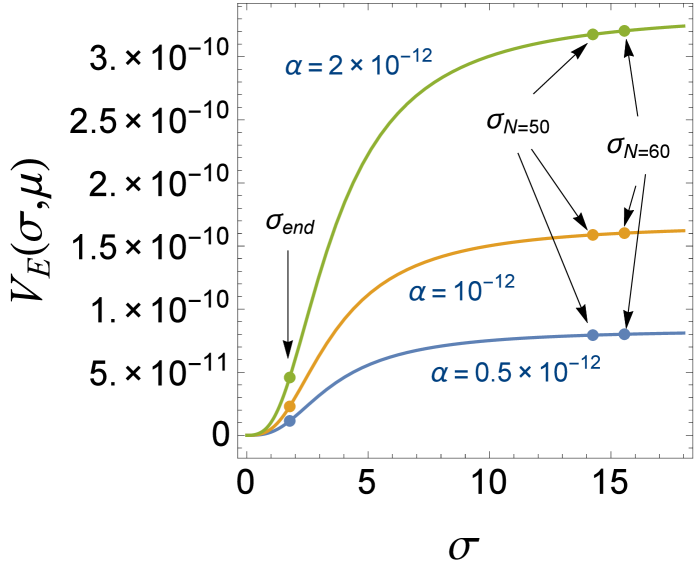
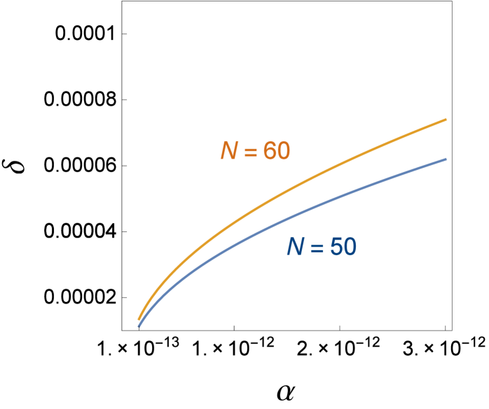
In this subsection we consider a model with a small number of fermion species, Nf=1,Nc=10formulae-sequencesubscript𝑁𝑓1subscript𝑁𝑐10N_{f}=1,\,N_{c}=10. First we set model parameters as 1/g4R1/g4R=1,μ=1,formulae-sequence1subscript𝑔4𝑅1superscriptsubscript𝑔4𝑅1𝜇11/g_{4R}-1/g_{4R}^{*}=1,\,\mu=1, and study the gauge coupling dependence. The behavior of the effective potential is drawn in Fig. 2 for α=0.5×1012,1×1012𝛼0.5superscript10121superscript1012\alpha=0.5\times 10^{-12},1\times 10^{-12} and 2×10122superscript10122\times 10^{-12}. We plot the points, σ=σend𝜎subscript𝜎𝑒𝑛𝑑\sigma=\sigma_{end}, σ=σN=50𝜎subscript𝜎𝑁50\sigma=\sigma_{N=50} and σ=σN=60𝜎subscript𝜎𝑁60\sigma=\sigma_{N=60} on each lines. A gentler slope of the potential is observed for a weaker gauge coupling. It should be noticed that we have to fine-tune the field configuration at the horizon crossing to obtain the enough e-foldings in the case of the NJL model (See Appendix A). The density fluctuation decreases as the slope becomes gentle. As is shown in Fig. 2, the density fluctuation is monotonically increasing as a function of α𝛼\alpha. The observed density fluctuation δ4.93×10⁵similar-to𝛿4.93superscript105\delta\sim 4.93\times 10^{-5} is obtained for αO(1012)similar-to𝛼𝑂superscript1012\alpha\sim O(10^{-12}).

Refer to caption
Figure 1: Behavior of the potential VE(σ,μ)subscript𝑉𝐸𝜎𝜇V_{E}(\sigma,\mu) as a function of σ𝜎\sigma for Nf=1subscript𝑁𝑓1N_{f}=1, Nc=10subscript𝑁𝑐10N_{c}=10, 1/g4R1/g4R=11subscript𝑔4𝑅1superscriptsubscript𝑔4𝑅11/g_{4R}-1/g_{4R}^{*}=1, μ=1𝜇1\mu=1 and α=0.5×1012,1×1012,2×1012𝛼0.5superscript10121superscript10122superscript1012\alpha=0.5\times 10^{-12},1\times 10^{-12},2\times 10^{-12}.
Refer to caption
Figure 2: Behavior of the density fluctuation δ𝛿\delta as a function of α𝛼\alpha for Nf=1subscript𝑁𝑓1N_{f}=1, Nc=10subscript𝑁𝑐10N_{c}=10, 1/g4R1/g4R=11subscript𝑔4𝑅1superscriptsubscript𝑔4𝑅11/g_{4R}-1/g_{4R}^{*}=1 and μ=1𝜇1\mu=1.

In Table 1 the values for the inflationary parameters nssubscript𝑛𝑠n_{s}, r𝑟r and αssubscript𝛼𝑠\alpha_{s} for α=1012,1011𝛼superscript1012superscript1011\alpha=10^{-12},10^{-11} and 1010superscript101010^{-10} are shown. The spectrum index nssubscript𝑛𝑠n_{s}, tensor-scalar ratio r𝑟r, and the running of the spectral index, αssubscript𝛼𝑠\alpha_{s}, are consistent with the observed Planck constraints, ns=0.9655±0.0062subscript𝑛𝑠plus-or-minus0.96550.0062n_{s}=0.9655\pm 0.0062, αs=0.0084±0.0082subscript𝛼𝑠plus-or-minus0.00840.0082\alpha_{s}=-0.0084\pm 0.0082 (68% CL, PlanckTT+lowP) and r0.002<0.10subscript𝑟0.0020.10r_{0.002}<0.10 (95% CL, PlanckTT+lowP)[7]. It is also found that the α𝛼\alpha-dependence for the inflationary parameters nssubscript𝑛𝑠n_{s}, r𝑟r and αssubscript𝛼𝑠\alpha_{s} is negligible.

α𝛼\alpha δ𝛿\delta nssubscript𝑛𝑠n_{s} r𝑟r αssubscript𝛼𝑠\alpha_{s}
1012superscript101210^{-12} 3.58×1053.58superscript1053.58\times 10^{-5} 0.961 0.0084 -0.00077
1011superscript101110^{-11} 1.13×1041.13superscript1041.13\times 10^{-4} 0.961 0.0084 -0.00077
1010superscript101010^{-10} 3.58×1043.58superscript1043.58\times 10^{-4} 0.961 0.0084 -0.00077
Table 1: Inflationary parameters for Nf=1subscript𝑁𝑓1N_{f}=1, Nc=10subscript𝑁𝑐10N_{c}=10, 1/g4R1/g4R=11subscript𝑔4𝑅1superscriptsubscript𝑔4𝑅11/g_{4R}-1/g_{4R}^{*}=1, μ=1𝜇1\mu=1 and N=50𝑁50N=50.

Next we discuss the dependence on the renormalized four-fermion coupling, g4Rsubscript𝑔4𝑅g_{4R} and the renormalization scale, μ𝜇\mu. Since a realistic value for the density fluctuation is obtained for αO(1012)similar-to𝛼𝑂superscript1012\alpha\sim O(10^{-12}), we set α=1012𝛼superscript1012\alpha=10^{-12} and numerically calculate the inflationary parameters as μ𝜇\mu and g4Rsubscript𝑔4𝑅g_{4R} vary. We show some typical values in Table 2. The μ𝜇\mu and g4Rsubscript𝑔4𝑅g_{4R} dependences are also negligible for the density fluctuation, δ𝛿\delta, the spectral index, nssubscript𝑛𝑠n_{s}, the tensor-to-scalar ratio, r𝑟r, and the running of the spectral index, αssubscript𝛼𝑠\alpha_{s}.

μ𝜇\mu 1/g4R1/g4R1subscript𝑔4𝑅1superscriptsubscript𝑔4𝑅1/g_{4R}-1/g_{4R}^{*} δ𝛿\delta nssubscript𝑛𝑠n_{s} r𝑟r αssubscript𝛼𝑠\alpha_{s}
108superscript10810^{-8} 1 3.59×1053.59superscript1053.59\times 10^{-5} 0.961 0.0083 -0.00076
104superscript10410^{-4} 1 3.59×1053.59superscript1053.59\times 10^{-5} 0.961 0.0083 -0.00076
1 1 3.58×1053.58superscript1053.58\times 10^{-5} 0.961 0.0084 -0.00077
1 104superscript10410^{-4} 3.59×1053.59superscript1053.59\times 10^{-5} 0.961 0.0083 -0.00076
1 108superscript10810^{-8} 3.59×1053.59superscript1053.59\times 10^{-5} 0.961 0.0083 -0.00076
Table 2: Inflationary parameters for Nf=1subscript𝑁𝑓1N_{f}=1, Nc=10subscript𝑁𝑐10N_{c}=10, α=1012𝛼superscript1012\alpha=10^{-12} and N=50𝑁50N=50.

It is found that the spectral index, the tensor-to-scalar ratio and the running of the spectral index are almost fixed at ns=0.961subscript𝑛𝑠0.961n_{s}=0.961, r=0.0083𝑟0.0083r=0.0083, αs=0.00076subscript𝛼𝑠0.00076\alpha_{s}=-0.00076 for N=50𝑁50N=50 in Nf=1subscript𝑁𝑓1N_{f}=1, Nc=10subscript𝑁𝑐10N_{c}=10 case. These values are consistent with the Planck 2015 data.

4.2 Large number of fermion species

Let us investigate the inflationary parameters at fixed gauge coupling limit, b+0𝑏0b\rightarrow+0 for simplicity. The assumption is valid for 11Nc2Nfsimilar-to11subscript𝑁𝑐2subscript𝑁𝑓11N_{c}\sim 2N_{f}. However, we vary the number of the fermion species, Nfsubscript𝑁𝑓N_{f} and Ncsubscript𝑁𝑐N_{c} , with a fixed gauge coupling, g𝑔g. Since the extremely small gauge coupling, αO(1012)similar-to𝛼𝑂superscript1012\alpha\sim O(10^{-12}), is considered the running of the gauge coupling in Eq. (2.5) can be neglected. The effective potential develops a non-trivial extremum for NfNc>24π2subscript𝑁𝑓subscript𝑁𝑐24superscript𝜋2N_{f}N_{c}>24\pi^{2} at the small gauge coupling limit. It induces the fine-tuning problem discussed in App. A. In order to avoid the problem we consider the limited case NfNc<24π2subscript𝑁𝑓subscript𝑁𝑐24superscript𝜋2N_{f}N_{c}<24\pi^{2}.

Refer to caption
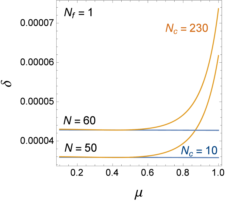
Figure 3: Behavior of the density fluctuation δ𝛿\delta as a function of μ𝜇\mu for Nf=1subscript𝑁𝑓1N_{f}=1, α=1012𝛼superscript1012\alpha=10^{-12}, 1/g4R1/g4R=11subscript𝑔4𝑅1superscriptsubscript𝑔4𝑅11/g_{4R}-1/g_{4R}^{*}=1.
Refer to caption
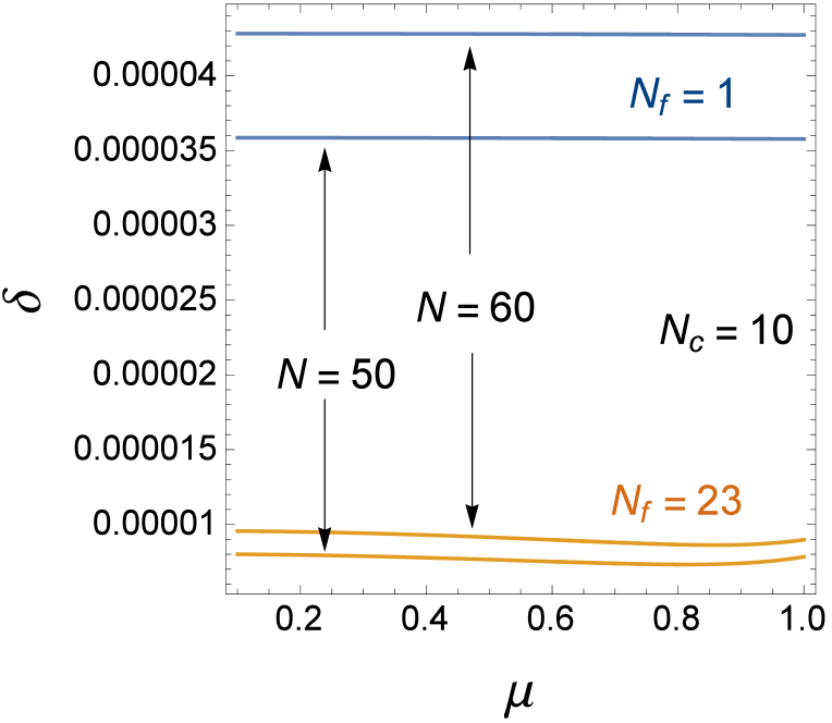
Figure 4: Behavior of the density fluctuation δ𝛿\delta as a function of μ𝜇\mu for Nc=10subscript𝑁𝑐10N_{c}=10, α=1012𝛼superscript1012\alpha=10^{-12}, 1/g4R1/g4R=11subscript𝑔4𝑅1superscriptsubscript𝑔4𝑅11/g_{4R}-1/g_{4R}^{*}=1.

In Figs. 4 and 4 we compare the behavior of the density fluctuation between a small and a large number of fermion species. The density fluctuation grows up near μ=1𝜇1\mu=1 for {Nf,Nc}={1,230}subscript𝑁𝑓subscript𝑁𝑐1230\{N_{f},N_{c}\}=\{1,230\} and {10,23}1023\{10,23\} cases. Non-negligible μ𝜇\mu dependence appears for a larger Nfsubscript𝑁𝑓N_{f} or Ncsubscript𝑁𝑐N_{c} cases. As is shown in Fig. 4 the obtained density fluctuation for Nc=230subscript𝑁𝑐230N_{c}=230 approaches to the one for Nc=10subscript𝑁𝑐10N_{c}=10 as the renormalization scale μ𝜇\mu decreases. We note that lines for Nc=10subscript𝑁𝑐10N_{c}=10 and Nc=230subscript𝑁𝑐230N_{c}=230 cross twice in μ[0,1]𝜇01\mu\in[0,1] and a small but a finite difference remains at μ0𝜇0\mu\rightarrow 0 limit. In Fig. 4 lines for Nf=1subscript𝑁𝑓1N_{f}=1 and Nf=23subscript𝑁𝑓23N_{f}=23 do not cross in μ[0,1]𝜇01\mu\in[0,1] and a larger difference observed at the limit, μ0𝜇0\mu\rightarrow 0.

Refer to caption
Refer to caption
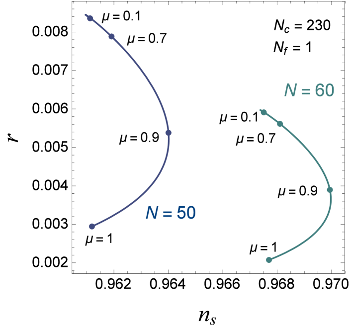
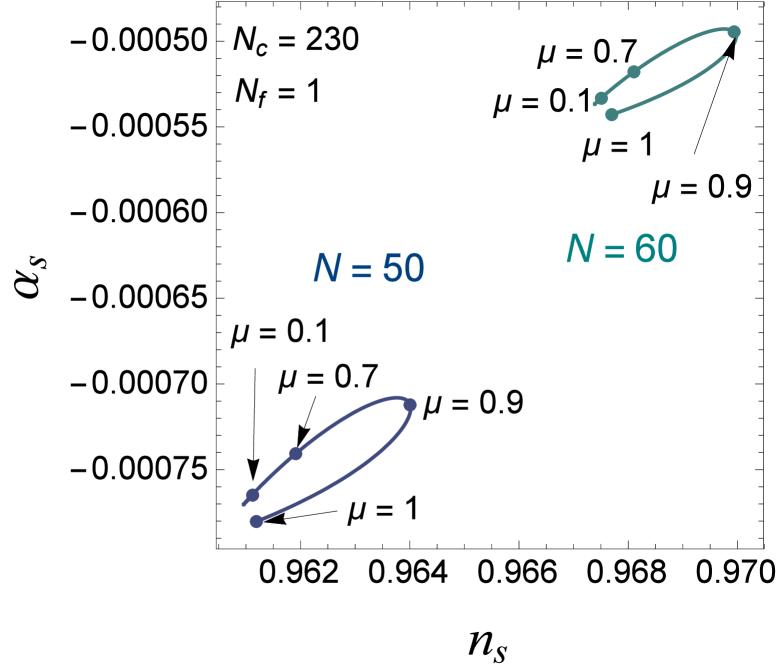
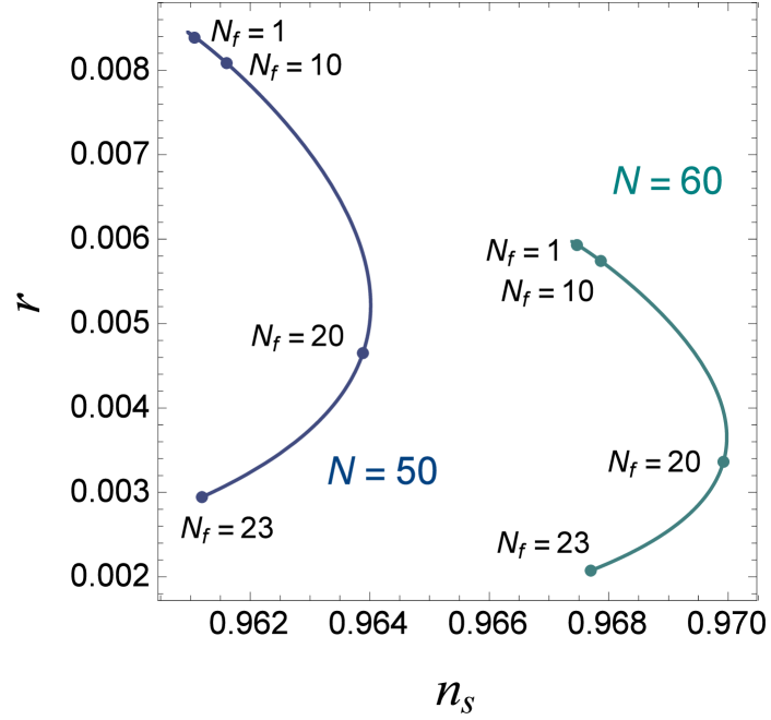
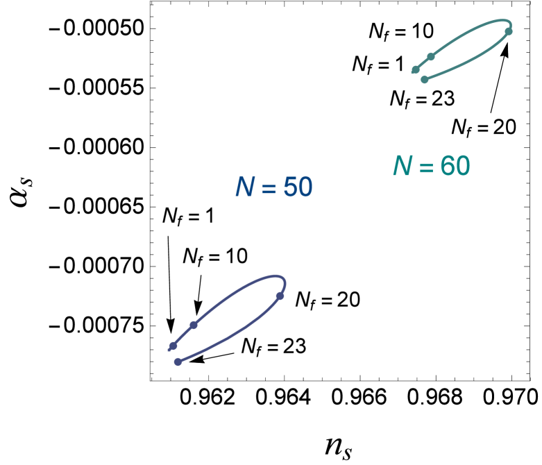
Figure 5: Behavior of the tensor-to-scalar ratio r𝑟r and the running of the spectral index αssubscript𝛼𝑠\alpha_{s} as a function of the spectral index nssubscript𝑛𝑠n_{s} for α=1012𝛼superscript1012\alpha=10^{-12}, Nf=1subscript𝑁𝑓1N_{f}=1, Nc=230subscript𝑁𝑐230N_{c}=230 and 1/g4R1/g4R=11subscript𝑔4𝑅1superscriptsubscript𝑔4𝑅11/g_{4R}-1/g_{4R}^{*}=1.
Refer to caption
Refer to caption
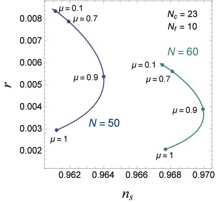
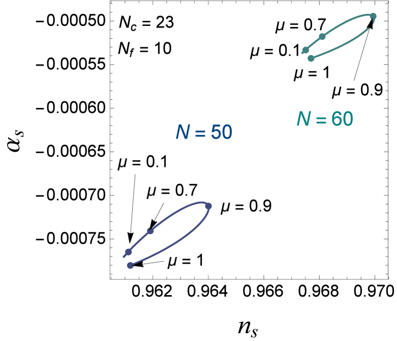
Figure 6: Behavior of the tensor-to-scalar ratio r𝑟r and the running of the spectral index αssubscript𝛼𝑠\alpha_{s} as a function of the spectral index nssubscript𝑛𝑠n_{s} for α=1012𝛼superscript1012\alpha=10^{-12}, Nf=10subscript𝑁𝑓10N_{f}=10, Nc=23subscript𝑁𝑐23N_{c}=23 and 1/g4R1/g4R=11subscript𝑔4𝑅1superscriptsubscript𝑔4𝑅11/g_{4R}-1/g_{4R}^{*}=1.

For a larger number of fermion species the μ𝜇\mu dependence appears in the spectral index, nssubscript𝑛𝑠n_{s}, the tensor-to-scalar ratio, r𝑟r, and the running of the spectral index, αssubscript𝛼𝑠\alpha_{s} in models. We draw the behavior of these inflationary parameters on the interval μ=[0.1,1.0]𝜇0.11.0\mu=[0.1,1.0] in Figs. 5 and 6. It should be noticed that we normalize the mass scale by the Planck scale and consider the large ΛΛ\Lambda limit. Such assumption is suitable for μ1.0Mpmuch-less-than𝜇1.0similar-tosubscript𝑀𝑝\mu\ll 1.0\sim M_{p}. A similar behavior is observed for {Nf,Nc}={1,230}subscript𝑁𝑓subscript𝑁𝑐1230\{N_{f},N_{c}\}=\{1,230\} and {10,23}1023\{10,23\} cases. Thus nssubscript𝑛𝑠n_{s}, r𝑟r and αssubscript𝛼𝑠\alpha_{s} seem to depend on the product NfNcsubscript𝑁𝑓subscript𝑁𝑐N_{f}N_{c}. At the limit, μ0𝜇0\mu\rightarrow 0, the result approaches to the one for a small number of fermion species, Nf=1subscript𝑁𝑓1N_{f}=1 and Nc=23subscript𝑁𝑐23N_{c}=23. The obtained trajectories are shifted as the e-folding number varies. All the trajectories are consistent with the Planck 2015 observations.
Refer to caption
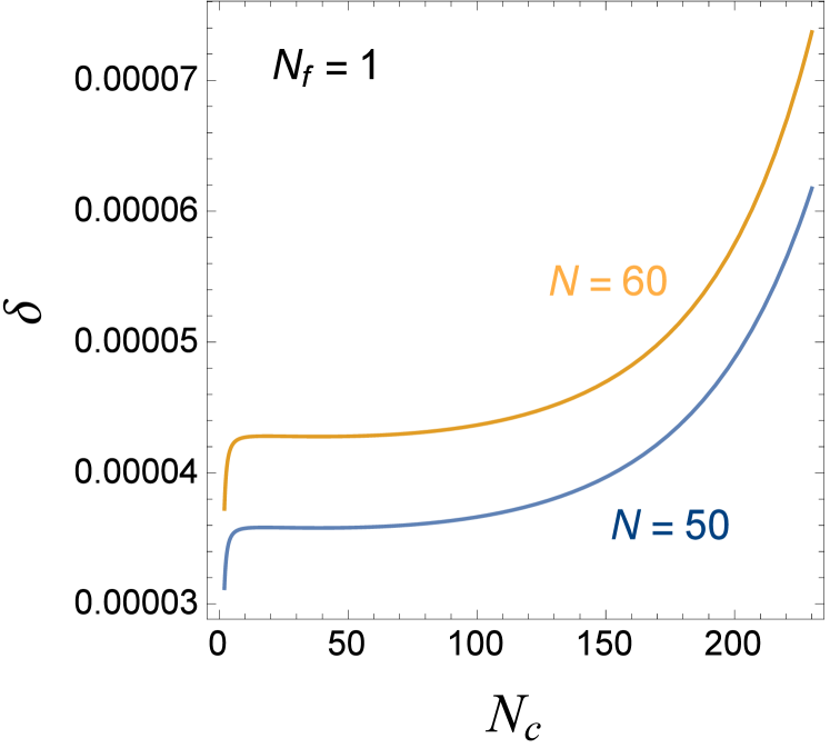
Figure 7: Behavior of the density fluctuation δ𝛿\delta as a function of Ncsubscript𝑁𝑐N_{c} for Nf=1subscript𝑁𝑓1N_{f}=1, α=1012𝛼superscript1012\alpha=10^{-12}, 1/g4R1/g4R=11subscript𝑔4𝑅1superscriptsubscript𝑔4𝑅11/g_{4R}-1/g_{4R}^{*}=1 and μ=1𝜇1\mu=1.
Refer to caption
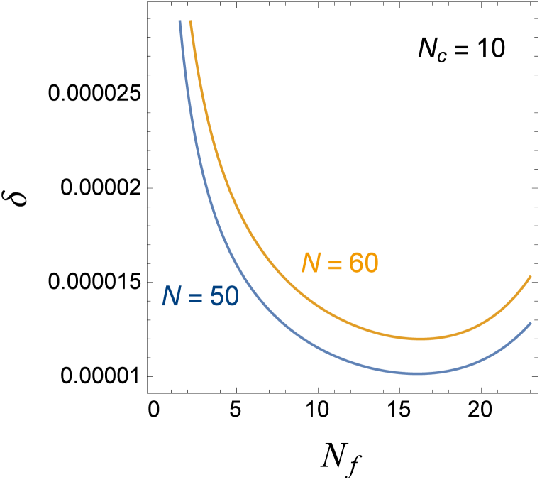
Figure 8: Behavior of the density fluctuation δ𝛿\delta as a function of Nfsubscript𝑁𝑓N_{f} for Nc=10subscript𝑁𝑐10N_{c}=10, α=1012𝛼superscript1012\alpha=10^{-12}, 1/g4R1/g4R=11subscript𝑔4𝑅1superscriptsubscript𝑔4𝑅11/g_{4R}-1/g_{4R}^{*}=1 and μ=1𝜇1\mu=1.

The inflationary parameters depend on the renormalization scale μ𝜇\mu for a larger number of the fermion species. It is observed that the parameters, nssubscript𝑛𝑠n_{s}, r𝑟r and αssubscript𝛼𝑠\alpha_{s} simply approach to the values for a small number of the fermion species at the small μ𝜇\mu limit. Next we fix the model parameters at μ=1𝜇1\mu=1, α=1012𝛼superscript1012\alpha=10^{-12}, 1/g4R1/g4R=11subscript𝑔4𝑅1superscriptsubscript𝑔4𝑅11/g_{4R}-1/g_{4R}^{*}=1 and evaluate the Nfsubscript𝑁𝑓N_{f} and Ncsubscript𝑁𝑐N_{c} dependences. The behavior of the density fluctuation, δ𝛿\delta, is plotted as Ncsubscript𝑁𝑐N_{c} and Nfsubscript𝑁𝑓N_{f} vary in Figs. 8 and 8, respectively. The range of the density fluctuation is smaller than the one in Fig. 2. The number of the fermion species induces a sub-dominant contribution to the density fluctuation compared with the gauge coupling. Thus, we can obtain a suitable density fluctuation by tuning the strength of the gauge coupling.
Refer to caption
Refer to caption
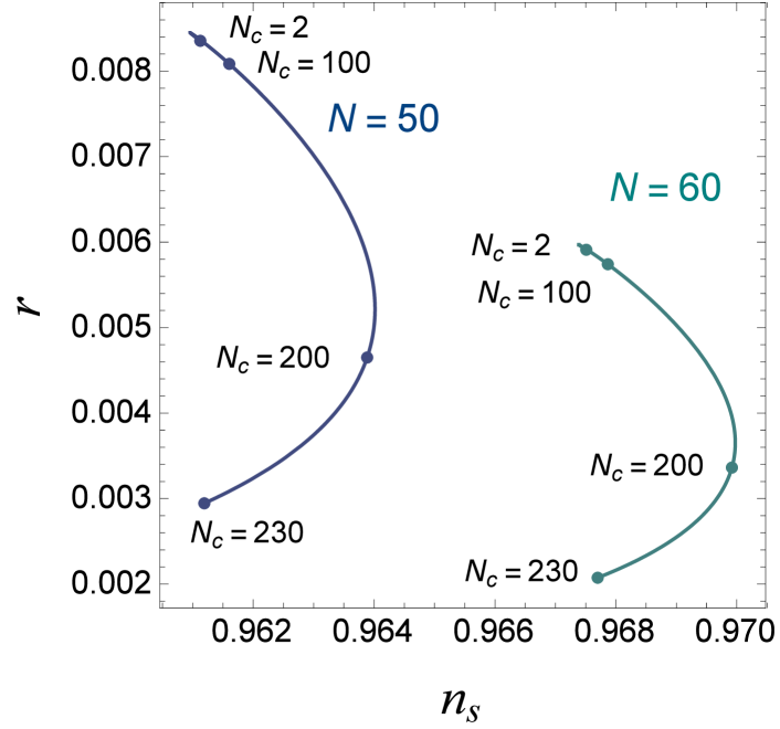
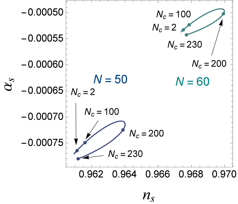
Figure 9: Behavior of the tensor-to-scalar ratio r𝑟r and the running of the spectral index αssubscript𝛼𝑠\alpha_{s} as a function of the spectral index nssubscript𝑛𝑠n_{s} for α=1012𝛼superscript1012\alpha=10^{-12}, Nf=1subscript𝑁𝑓1N_{f}=1, 1/g4R1/g4R=11subscript𝑔4𝑅1superscriptsubscript𝑔4𝑅11/g_{4R}-1/g_{4R}^{*}=1 and μ=1𝜇1\mu=1.
Refer to caption
Refer to caption
Figure 10: Behavior of the tensor-to-scalar ratio r𝑟r and the running of the spectral index αssubscript𝛼𝑠\alpha_{s} as a function of the spectral index nssubscript𝑛𝑠n_{s} for α=1012𝛼superscript1012\alpha=10^{-12}, Nc=10subscript𝑁𝑐10N_{c}=10, 1/g4R1/g4R=11subscript𝑔4𝑅1superscriptsubscript𝑔4𝑅11/g_{4R}-1/g_{4R}^{*}=1 and μ=1𝜇1\mu=1.

In Figs. 9 and 10 the tensor-to-scalar ratio, r𝑟r, and the running of the spectral index, αssubscript𝛼𝑠\alpha_{s}, are plotted as functions of the spectral index, nssubscript𝑛𝑠n_{s}, for the e-folding number, N=50𝑁50N=50 and 606060. Both the figures show a similar behavior to Figs. 5 and 6. A model with a large number of fermion species at μ1similar-to𝜇1\mu\sim 1 and a small number of fermion species at a small μ𝜇\mu generate nearly equal values of nssubscript𝑛𝑠n_{s}, r𝑟r and αssubscript𝛼𝑠\alpha_{s}. The obtained trajectories are consistent with the Planck 2015 results. The tensor-to-scalar ratio, r𝑟r, monotonically decreases as Ncsubscript𝑁𝑐N_{c} and Nfsubscript𝑁𝑓N_{f} increases. The spectral index, nssubscript𝑛𝑠n_{s} and the running of the spectral index, αssubscript𝛼𝑠\alpha_{s} have maximal values at a=2NfNc380𝑎2subscript𝑁𝑓subscript𝑁𝑐similar-to380a=2N_{f}N_{c}\sim 380.

Thus, we demonstrated that realistic gauged NJL-model under discussion for specific values of parameters is consistent with Planck cosmological data. From another side, the model under discussion is realistic high energy physics model of elementary particles. For numerical calculations, we considered several choices of fermion species so that such choice is quite standard in particle physics. Thus, we arrive to realistic (composite) particle physics model which predicts viable inflation.

5 Exit from inflation

The end of the slow roll era is found by observing the parameters, ϵitalic-ϵ\epsilon and η𝜂\eta. In the present model the parameter ϵitalic-ϵ\epsilon exceeds unity at σ=σend𝜎subscript𝜎𝑒𝑛𝑑\sigma=\sigma_{end} in Fig. 2. Under the slow roll approximation, the deceleration parameter, q𝑞q, is written as

qa¨H2aϵ1.𝑞¨𝑎superscript𝐻2𝑎similar-toitalic-ϵ1\displaystyle q\equiv-\frac{\ddot{a}}{H^{2}a}\sim\epsilon-1. (5.1)

The deceleration parameter changes the sign at σ=σend𝜎subscript𝜎𝑒𝑛𝑑\sigma=\sigma_{end} and develops a positive value. Thus the universe turns to decelerated expansion era.

In this paper we set the initial condition σNsubscript𝜎𝑁\sigma_{N} to generate the e-folding number between 50 and 60. Thus the duration of the inflation can be estimated by

tduration=σendσN(σφ)23VEVE/σ𝑑σ.subscript𝑡𝑑𝑢𝑟𝑎𝑡𝑖𝑜𝑛superscriptsubscriptsubscript𝜎𝑒𝑛𝑑subscript𝜎𝑁superscript𝜎𝜑23subscript𝑉𝐸subscript𝑉𝐸𝜎differential-d𝜎\displaystyle t_{duration}=\int_{\sigma_{end}}^{\sigma_{N}}\left(\frac{\partial\sigma}{\partial\varphi}\right)^{2}\frac{\sqrt{3V_{E}}}{\partial V_{E}/\partial\sigma}d\sigma. (5.2)

We numerically find

tduration=(78)×106Mp11036s.subscript𝑡𝑑𝑢𝑟𝑎𝑡𝑖𝑜𝑛similar-to78superscript106superscriptsubscript𝑀𝑝1similar-tosuperscript1036s\displaystyle t_{duration}=(7\sim 8)\times 10^{6}M_{p}^{-1}\sim 10^{-36}\,\mbox{s}. (5.3)

From Eqs. (3.8) and (3.9) we obtain

H2=13(H˙+VE).superscript𝐻213˙𝐻subscript𝑉𝐸\displaystyle H^{2}=\frac{1}{3}(-\dot{H}+V_{E}). (5.4)

We define the perturbation ΔH(t)Δ𝐻𝑡\Delta H(t) by

H=HdS+ΔH(t),𝐻subscript𝐻𝑑𝑆Δ𝐻𝑡\displaystyle H=H_{dS}+\Delta H(t), (5.5)

with HdSVE/3subscript𝐻𝑑𝑆subscript𝑉𝐸3H_{dS}\equiv V_{E}/3. Inserting Eq. (5.5) into Eq. (5.4), we get

ΔH˙ΔH6HdS+O(ΔH2).similar-toΔ˙𝐻Δ𝐻6subscript𝐻𝑑𝑆OΔsuperscript𝐻2\displaystyle\frac{\Delta\dot{H}}{\Delta H}\sim-6H_{dS}+\mbox{O}(\Delta H^{2}). (5.6)

The solution of this equation is given by

ΔH(t)=Asinh(6V3t),Δ𝐻𝑡𝐴6𝑉3𝑡\displaystyle\Delta H(t)=A\sinh\left(6\sqrt{\frac{V}{3}}t\right), (5.7)

where we set an initial condition ΔH(t=0)=0Δ𝐻𝑡00\Delta H(t=0)=0 and A𝐴A is a constant parameter. Thus the de Sitter solution (3.11) is unstable. As is shown in Fig. 2, the potential energy extremely decreases at σ=σend𝜎subscript𝜎𝑒𝑛𝑑\sigma=\sigma_{end}. Then the dominant contribution to derive the expansion of the universe comes from the radiation. Therefore, the standard cosmology is recovered. It should be noted that R2superscript𝑅2R^{2} terms induced by the trace anomaly also unstabilizes the de Sitter solution and then the radiation dominant era realizes [23].

6 Conclusions

In summary, we proposed gauged NJL inflation as an alternative for Higgs inflation. Specifically, the gauged NJL model is studied as the realistic particle physics model for the composite scalar. Applying the auxiliary field method and performing the renormalization group improvement (for review of RG in curved spacetime, see [21]), the model is represented by the gauge-Higgs-Yukawa theory. We assumed that the gauge-Higgs-Yukawa theory well describes the model at the scale of inflation at the ΛΛ\Lambda\rightarrow\infty limit. Then the produced CMB fluctuations have been calculated in the gauge-Higgs-Yukawa theory with the compositeness conditions at the fixed gauge coupling.

The behavior for inflationary parameters δ𝛿\delta, nssubscript𝑛𝑠n_{s}, r𝑟r and αssubscript𝛼𝑠\alpha_{s} has been numerically evaluated as a function of the couplings, the renormalization scale, the e-folding number and the number of the fermion species. It is found that the smallness of the density fluctuation can be realized by tuning the gauge coupling. We proved that the model with a small number of fermion species, Nf=1,Nc=10formulae-sequencesubscript𝑁𝑓1subscript𝑁𝑐10N_{f}=1,\,N_{c}=10 satisfies the Planck 2015 data. In this case the spectral index, the tensor-to-scalar ratio and the running of the spectral index develop almost fixed values, ns=0.961subscript𝑛𝑠0.961n_{s}=0.961, r=0.0083𝑟0.0083r=0.0083, αs=0.00076subscript𝛼𝑠0.00076\alpha_{s}=-0.00076 for N=50𝑁50N=50. For a large number of fermion species, these inflationary parameters depend on the renormalization scale μ𝜇\mu. However, the obtained trajectories of the inflationary parameters are consistent with the Planck 2015 data. Therefore, the gauged NJL model naturally generates inflationary parameters consistent with the Planck 2015 observation and may serve as viable inflationary theory.

At the next step, one has to consider the end of inflation and graceful exit. It is clear that higher-derivative RG corrected terms (like R2superscript𝑅2R^{2}, etc) which are induced as vacuum polarization beyond the linear-curvature approximation may naturally provide the graceful exit. It is also interesting to consider the reheating process in the gauged NJL model. In fact, this goes beyond this work. However, the preliminary considerations of preheating process indicate reheating maybe successful as it is in usual scalar theories of inflation (in fact, our model is effectively scalar inflationary theory). These questions will be considered elsewhere. Furthermore, NJL model may pretend to the role of dark matter (see, for instance, Ref. [22]), hence presumably unifying inflation with dark matter.

Acknowledgements

The authors are grateful to T. Kugo for useful comments. The work by TI is supported in part by JSPS KAKENHI Grant Number 26400250 and that by SDO is supported in part by MINECO (Spain), project FIS2013-44881 and by MES (Russia).

Appendix A NJL limit

Let us discuss the slow-roll solution in the NJL model. It is obtained by omitting the gauge interaction. Here we consider the NJL limit, α0𝛼0\alpha\to 0, where the gauge interaction is eliminated. At the limit the running couplings (2.9) and (2.10) reduce to

yΛ2(t)=16π22aααc[1(μ2Λ2)1w]1=16π22a2ln(μ2/Λ2),superscriptsubscript𝑦Λ2𝑡16superscript𝜋22𝑎𝛼subscript𝛼𝑐superscriptdelimited-[]1superscriptsuperscript𝜇2superscriptΛ21𝑤116superscript𝜋22𝑎2superscript𝜇2superscriptΛ2\displaystyle y_{\Lambda}^{2}(t)=\frac{16\pi^{2}}{2a}\frac{\alpha}{\alpha_{c}}\left[1-\left(\frac{\mu^{2}}{\Lambda^{2}}\right)^{1-w}\right]^{-1}=-\frac{16\pi^{2}}{2a}\frac{2}{\ln(\mu^{2}/\Lambda^{2})}, (A.1)
λΛ(t)yΛ4(t)=2a16π2αcα[1(μ2Λ2)22w]=2a16π2ln(μ2/Λ2).subscript𝜆Λ𝑡superscriptsubscript𝑦Λ4𝑡2𝑎16superscript𝜋2subscript𝛼𝑐𝛼delimited-[]1superscriptsuperscript𝜇2superscriptΛ222𝑤2𝑎16superscript𝜋2superscript𝜇2superscriptΛ2\displaystyle\frac{\lambda_{\Lambda}(t)}{y_{\Lambda}^{4}(t)}=\frac{2a}{16\pi^{2}}\frac{\alpha_{c}}{\alpha}\left[1-\left(\frac{\mu^{2}}{\Lambda^{2}}\right)^{2-2w}\right]=-\frac{2a}{16\pi^{2}}\ln(\mu^{2}/\Lambda^{2}). (A.2)

From Eqs. (2.14) and (A.1) we obtain

m2(t)=2a16π2(Λ2μ2)wyΛ2(t)μ2(1g4(Λ)1w)Λμ2(1g4R(μ)1g4R),superscript𝑚2𝑡2𝑎16superscript𝜋2superscriptsuperscriptΛ2superscript𝜇2𝑤subscriptsuperscript𝑦2Λ𝑡superscript𝜇21subscript𝑔4Λ1𝑤Λsuperscript𝜇21subscript𝑔4𝑅𝜇1superscriptsubscript𝑔4𝑅\displaystyle m^{2}(t)=\frac{2a}{16\pi^{2}}\left(\frac{\Lambda^{2}}{\mu^{2}}\right)^{w}y^{2}_{\Lambda}(t)\mu^{2}\left(\frac{1}{g_{4}(\Lambda)}-\frac{1}{w}\right)\xrightarrow{\Lambda\to\infty}\mu^{2}\left(\frac{1}{g_{4R}(\mu)}-\frac{1}{g_{4R}^{*}}\right), (A.3)

where we renormalize g4(Λ)subscript𝑔4Λg_{4}(\Lambda) suitably to obtain a finite expression [16].

Following the similar procedure in Sec. 2 we calculate the RG invariant effective potential at the limit ΛΛ\Lambda\to\infty and obtain

V(σ)=12(1g4R1g4R)μ2σ2+R12σ2.𝑉𝜎121subscript𝑔4𝑅1superscriptsubscript𝑔4𝑅superscript𝜇2superscript𝜎2𝑅12superscript𝜎2\displaystyle V(\sigma)=\frac{1}{2}\left(\frac{1}{g_{4R}}-\frac{1}{g_{4R}^{*}}\right)\mu^{2}\sigma^{2}+\frac{R}{12}\sigma^{2}. (A.4)

Thus, the gravitational effective action with the weak curvature Rσ2much-less-than𝑅superscript𝜎2R\ll\sigma^{2} becomes

S(NJL)=d4xg[12R+12gμνμσνσV(σ)].superscript𝑆𝑁𝐽𝐿superscript𝑑4𝑥𝑔delimited-[]12𝑅12superscript𝑔𝜇𝜈subscript𝜇𝜎subscript𝜈𝜎𝑉𝜎\displaystyle S^{(NJL)}=\int d^{4}x\sqrt{-g}\left[-\frac{1}{2}R+\frac{1}{2}g^{\mu\nu}\partial_{\mu}\sigma\partial_{\nu}\sigma-V(\sigma)\right]. (A.5)

By the Weyl transformation (3.1), one can eliminate the interaction term between the curvature and the auxiliary field σ𝜎\sigma. In the Einstein frame the action is simplified as

SE(NJL)=d4xg~[12R~+12g~μνμφνφVE(σ)],subscriptsuperscript𝑆𝑁𝐽𝐿𝐸superscript𝑑4𝑥~𝑔delimited-[]12~𝑅12superscript~𝑔𝜇𝜈subscript𝜇𝜑subscript𝜈𝜑subscript𝑉𝐸𝜎\displaystyle S^{(NJL)}_{E}=\int d^{4}x\sqrt{-\tilde{g}}\left[-\frac{1}{2}\tilde{R}+\frac{1}{2}\tilde{g}^{\mu\nu}\partial_{\mu}\varphi\partial_{\nu}\varphi-V_{E}(\sigma)\right], (A.6)

with the effective potential

VE(σ)=12[1g4R1g4R]μ2σ2(1+σ2/6)2.subscript𝑉𝐸𝜎12delimited-[]1subscript𝑔4𝑅1superscriptsubscript𝑔4𝑅superscript𝜇2superscript𝜎2superscript1superscript𝜎262\displaystyle V_{E}(\sigma)=\frac{1}{2}\left[\frac{1}{g_{4R}}-\frac{1}{g_{4R}^{*}}\right]\frac{\mu^{2}\sigma^{2}}{(1+\sigma^{2}/6)^{2}}. (A.7)

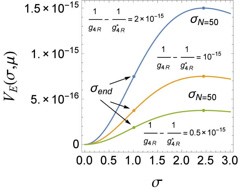
The denominator (1+σ2/6)2superscript1superscript𝜎262(1+\sigma^{2}/6)^{2} comes from the NJL limit of Ω2superscriptΩ2\Omega^{2} in Eq. (3.2). It suppresses the effective potential for a large σ𝜎\sigma. The effective potential (A.7) has a maximum at σ=6𝜎6\sigma=\sqrt{6}.

Refer to caption
Figure 11: Behavior of the potential VE(σ)subscript𝑉𝐸𝜎V_{E}(\sigma) as a function of σ𝜎\sigma for μ=1𝜇1\mu=1 and 1/g4R1/g4R=0.5×1015,1×1015,2×10151subscript𝑔4𝑅1superscriptsubscript𝑔4𝑅0.5superscript10151superscript10152superscript10151/g_{4R}-1/g_{4R}^{*}=0.5\times 10^{-15},1\times 10^{-15},2\times 10^{-15}. It should be noticed that we do not adopt any model parameters whose effective potential has a local maximum except for this appendix.
Refer to caption
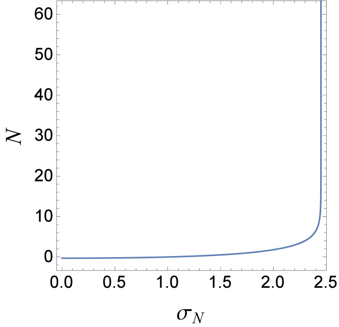
Figure 12: Behavior of the e-folding number N𝑁N as a function of σNsubscript𝜎𝑁\sigma_{N}.

In Fig. 12 the typical behavior of the effective potential (A.7) is shown. It is observed that the horizon crossing σ=σN𝜎subscript𝜎𝑁\sigma=\sigma_{N} should take place near the maximum of the potential to obtain large enough e-folding N=5060𝑁50similar-to60N=50\sim 60. The e-folding is plotted as a function of σNsubscript𝜎𝑁\sigma_{N} in Fig. 12. It blows up at σ=6𝜎6\sigma=\sqrt{6}. We noted that the g4Rsubscript𝑔4𝑅g_{4R} dependence gives only a negligible contribution to the e-folding. The result introduces a fine- tuning problem why σN6similar-tosubscript𝜎𝑁6\sigma_{N}\sim\sqrt{6}. To avoid this fine-tuning problem one should modify the potential. Since the potential can be easily modified by including terms which are neglected in our approximation, the fine-tuning problem seems to be not so serious.

References

  • [1] Y. Nambu and G. Jona-Lasinio, Phys. Rev.  122 (1961) 345; Phys. Rev.  124 (1961) 246.
  • [2] V. A. Miransky, Dynamical Symmetry Breaking in Quantum Field Theories, World Scientific (1993);
    M. Harada and K. Yamawaki, Phys. Rept.  381 (2003) 1 [hep-ph/0302103].
  • [3] K.-I. Kondo, S. Shuto and K. Yamawaki, Mod. Phys. Lett. A6 (1991) 3385;
    K.-I. Kondo, M. Tanabashi and K. Yamawaki, Progr. Theor. Phys. 89 (1993) 1249; Mod. Phys. Lett. A8 (1993) 2859.
  • [4] C. N. Leung, S. T. Love and W. A. Bardeen, Nucl. Phys. B 273 (1986) 649; Nucl. Phys. B 323 (1989) 493.
  • [5] C. T. Hill and E. H. Simmons, Phys. Rept.  381 (2003) 235 [Phys. Rept.  390 (2004) 553] [hep-ph/0203079].
  • [6] P. A. R. Ade et al. [BICEP2 and Planck Collaborations], Phys. Rev. Lett.  114 (2015) 101301 [arXiv:1502.00612 [astro-ph.CO]].
  • [7] P. A. R. Ade et al. [Planck Collaboration], arXiv:1502.01589 [astro-ph.CO]. arXiv:1502.02114 [astro-ph.CO].
  • [8] T. Inagaki, T. Muta and S. D. Odintsov, Mod. Phys. Lett. A 8 (1993) 2117 [hep-th/9306023]; Prog. Theor. Phys. Suppl.  127 (1997) 93 [hep-th/9711084].
  • [9] C. T. Hill and D. S. Salopek, Annals Phys.  213 (1992) 21.
  • [10] T. Muta and S. D. Odintsov, Mod. Phys. Lett. A 6 (1991) 3641.
  • [11] B. Geyer and S. D. Odintsov, Phys. Lett. B 376 (1996) 260 [hep-th/9603172]; Phys. Rev. D 53 (1996) 7321 [hep-th/9602110].
  • [12] T. Inagaki, Y. Rybalov and X. Meng, Eur. Phys. J. C 71 (2011) 1656 [arXiv:1102.5036 [hep-ph]].
  • [13] S. Iso, K. Kohri and K. Shimada, Phys. Rev. D 91 (2015) 044006 [arXiv:1408.2339 [hep-ph]].
  • [14] E. Elizalde and S. D. Odintsov, Phys. Lett. B 303 (1993) 240 [hep-th/9302074]; Phys. Lett. B 321 (1994) 199 [hep-th/9311087];Z. Phys. C 64 (1994) 699 [hep-th/9401057].
  • [15] A. De Simone, M. P. Hertzberg and F. Wilczek, Phys. Lett. B 678 (2009) 1 [arXiv:0812.4946 [hep-ph]];
    S. Mukaigawa, T. Muta and S. D. Odintsov, Int. J. Mod. Phys. A 13 (1998) 2739 [hep-ph/9709299];
    H. M. Lee, Phys. Lett. B 722 (2013) 198 [arXiv:1301.1787 [hep-ph]];
    N. Okada and Q. Shafi, arXiv:1311.0921 [hep-ph]; G. Barenboim, E. J. Chun and H. M. Lee, Phys. Lett. B 730 (2014) 81;
    Y. Hamada, H. Kawai, K. y. Oda and S. C. Park, Phys. Rev. Lett.  112 (2014) 241301 [arXiv:1403.5043 [hep-ph]];
    R. P. Woodard, Phys. Rev. Lett.  101 (2008) 081301 [arXiv:0805.3089 [gr-qc]];
    I. Oda and T. Tomoyose, Adv. Stud. Theor. Phys.  8 (2014) 551 [arXiv:1404.1538 [hep-ph]];
    J. Ren, Z. Z. Xianyu and H. J. He, JCAP 1406 (2014) 032 [arXiv:1404.4627 [gr-qc]];
    Y. Hamada, H. Kawai and K. y. Oda, JHEP 1407 (2014) 026;
    T. Inagaki, R. Nakanishi and S. D. Odintsov, Astrophys. Space Sci.  354 (2014) 2108 [arXiv:1408.1270 [gr-qc]]; Phys. Lett. B 745 (2015) 105 [arXiv:1502.06301 [hep-ph]];
    E. Elizalde, S. D. Odintsov, E. O. Pozdeeva and S. Y. Vernov, Phys. Rev. D 90 (2014) 084001 [arXiv:1408.1285 [hep-th]];
    Y. Hamada, H. Kawai, K. y. Oda and S. C. Park, Phys. Rev. D 91 (2015) 053008 [arXiv:1408.4864 [hep-ph]];
    H. J. He and Z. Z. Xianyu, JCAP 1410 (2014) 019 [arXiv:1405.7331 [hep-ph]];
    M. Herranen, T. Markkanen, S. Nurmi and A. Rajantie, Phys. Rev. Lett.  113 (2014) 211102 [arXiv:1407.3141 [hep-ph]];
    M. Herranen, A. Osland and A. Tranberg, arXiv:1503.07661 [hep-ph].
  • [16] M. Harada, Y. Kikukawa, T. Kugo and H. Nakano, Prog. Theor. Phys.  92 (1994) 1161 [hep-ph/9407398].
  • [17] W. A. Bardeen, C. T. Hill and M. Lindner, Phys. Rev. D 41 (1990) 1647.
  • [18] D. I. Kaiser, Phys. Lett. B 340 (1994) 23 [astro-ph/9405029]; Phys. Rev. D 52 (1995) 4295 [astro-ph/9408044].
  • [19] A. D. Linde, Contemp. Concepts Phys.  5 (1990) 1 [hep-th/0503203];
    D. S. Gorbunov and V. A. Rubakov, “Introduction to the theory of the early universe: Cosmological perturbations and inflationary theory,” Hackensack, USA: World Scientific (2011) 489 p
  • [20] K. Kohri, Y. Oyama, T. Sekiguchi and T. Takahashi, JCAP 1310 (2013) 065 [arXiv:1303.1688 [astro-ph.CO]].
  • [21] I. L. Buchbinder, S. D. Odintsov, I. L. Shapiro, ”Effective Action in Quantum Gravity,” Bristol, UK: IOP (1992).
  • [22] M. Holthausen, J. Kubo, K. S. Lim and M. Lindner, JHEP 1312 (2013) 076 [arXiv:1310.4423 [hep-ph]].
  • [23] K. Bamba, R. Myrzakulov, S. D. Odintsov and L. Sebastiani, Phys. Rev. D 90 (2014) 043505 [arXiv:1403.6649 [hep-th]].