The connections between the UV and optical Fe II emission lines in type 1 AGNs

Abstract

We investigate the spectral properties of the UV ($\lambda\lambda$2650-3050 Å) and optical ($\lambda\lambda$4000-5500 Å) Fe II emission features in a sample of 293 type 1 active galactic nuclei (AGNs) from Sloan Digital Sky Survey (SDSS) database. We explore different correlations between their emission line properties, as well as the correlations with the other emission lines from the spectral range. We find several interesting correlations and we can outline the most interesting results as follows. (i) There is a kinematical connection between the UV and optical Fe II lines, indicating that the UV and optical Fe II lines originate from the outer part of the broad line region, so-called intermediate line region; (ii) The unexplained anticorrelations of the optical Fe II (EW Fe II_opt) vsersus EW [O III] 5007 Å and EW Fe II_opt versus FWHM H$\beta$ have not been detected for the UV Fe II lines; (iii) The significant averaged redshift in the UV Fe II lines, which is not present in optical Fe II, indicates an inflow in the UV Fe II emitting clouds, and probably their asymmetric distribution. (iv) Also, we confirm the anticorrelation between the intensity ratio of the optical and UV Fe II lines and FWHM of H$\beta$, and we find the anticorrelations of this ratio with the widths of Mg II 2800 Å, optical Fe II and UV Fe II. This indicates a very important role for the column density and microturbulence in the emitting gas. We discuss the starburst activity in high–density regions of young AGNs as a possible explanation of the detected optical Fe II correlations and intensity line ratios of the UV and optical Fe II lines.

1 Introduction

The spectral properties of active galactic nuclei (AGNs) depend on the physical conditions and geometry of emitting regions that radiate in a wide wavelength range. Among a large diversity of the spectral features in AGN spectra, iron lines are one of the most intriguing because there are numerous open questions about their nature (see, e.g., Collin & Joly, 2000). They can be very intense in the UV and optical part around Mg II $\lambda$2800 Å and H$\beta$. The mechanism of their excitation, the explanation of the observed Fe II strength, the place of the Fe II emission region in an AGN structure, and some correlations observed between Fe II and some other spectral properties are still a matter of debate (for detailed review see Kovačević et al., 2010).

It is widely accepted that the iron is mostly produced by the Type Ia supernovae after explosions of long-lived, intermediate-mass binaries. Therefore, it is expected that the ratio of Fe to some elements (O, N, Mg) that are produced in explosions of short-lived, massive stars (primarily Type II supernovae), could be a cosmological metallicity indicator, due to their different enrichment timescales (Verner et al., 2003); that is the iron lines may serve to constrain the age of an AGN and its host galaxy (see e.g. Dong et al., 2011; De Rosa et al., 2011, and references therein).

To understand the nature and evolution of AGNs, efforts have been made to investigate the correlations between the spectral properties in different AGN spectral bands and to determine the physics that is behind the detected correlations (see e.g. Boroson & Green, 1992; Wills et al., 1999; Croom et al., 2002; Shang et al., 2003; Yip et al., 2004; Grupe, 2004; Wang et al., 2006, 2009; Ludwig et al., 2009; Kovačević et al., 2010; Popović & Kovačević, 2011; Marchese et al., 2012; Grupe & Nousek, 2015, etc.). Some correlations between the optical Fe II and other spectral properties in AGNs have been reported, but the physical explanation is unknown (see Boroson & Green, 1992; Kovačević et al., 2010). Some of these correlations, for example, are part of Eigenvector 1 of Boroson & Green (1992) (for a review see Kovačević et al., 2010; Popović & Kovačević, 2011, and references therein). Among them, the most interesting are the anticorrelations of the equivalent widths (EW) Fe II optical lines with the EW [O III] and H$\beta$ width. However, it is difficult to determine the physics that is behind these correlations because choosing a sample of AGNs using different spectral criteria (continuum luminosity, [O III] strength, FWHM H$\beta$ etc.) can give different correlations between spectral properties, and in some cases even the opposite in different subsamples (Yip et al., 2004; Grupe, 2004; Ludwig et al., 2009; Sulentic et al., 2009; Popović & Kovačević, 2011). As an example, a significant difference is seen between the correlations in spectral properties for objects divided by FWHM of H$\beta$ (Sulentic et al., 2009; Kovačević et al., 2010). However, it seems that more relevant is to consider AGNs with different [O III] 5007 Å to narrow H$\beta$ ratios ($\mathrm{[OIII]}/\mathrm{H\beta}_{NLR}$), because this may give an additional information about the starburst (SB) fraction in AGNs (see Popović & Kovačević, 2011), which is probably related to the AGN evolution (Lípari & Terlevich, 2006; Mao et al., 2009; Sani et al., 2010; Popović & Kovačević, 2011). In an early phase of their evolution, AGNs are probably composite objects, which consist of SBs (star-forming regions) and the central AGN engine. The influence of SBs on the spectral properties becomes weaker in a later phase of the AGN evolution (Mao et al., 2009).

The origin of the iron lines is also very intriguing question. The mechanism of their excitation, the explanation of the observed Fe II strength, and the place of Fe II emission region in an AGN structure are still a matter of debate.

Several authors have shown that a classical photoionization model cannot sufficiently explain the observed UV and optical Fe II emission strengths, and that additional processes must be included (Collin-Souffrin et al., 1980; Joly, 1987; Sigut and Pradhan, 1998, 2003; Collin & Joly, 2000; Verner et al., 2003; Baldwin et al., 2004; Bruhweiler & Verner, 2008; Sameshima et al., 2011, etc.). There are some indications that microturbulence may have a significant influence on the Fe II strength (Netzer & Wills, 1983; Verner et al., 2003; Sigut and Pradhan, 2003; Baldwin et al., 2004; Bruhweiler & Verner, 2008; Sameshima et al., 2011). Baldwin et al. (2004) showed that a photoionization model may reproduce well the observed shape and the EW of the UV Fe II 2200-2800 bump, but only if a microturbulent gas motion is taken into account. The Fe II strength is also controlled by the column density as well (Joly, 1987; Verner et al., 2004; Ferland et al., 2009; Sameshima et al., 2011) and that the strong Fe II emission is connected with high density emitting regions (Joly, 1991; Baldwin et al., 1996; Lawrence et al., 1997; Kuraszkiewicz et al., 2000; Graham et al., 1996; Harris et al., 2013; Clowes et al., 2013).

It seems that there are significant differences in the physics of the UV Fe II and optical Fe II emission region: the optical and UV Fe II lines correlate differently with some physical properties. The $\mathrm{FeII}_{opt}/\mathrm{FeII}_{UV}$ ratio depends on column density (Joly, 1987; Sameshima et al., 2011) and microturbulence (Verner et al., 2003). Classical photoionization models, assuming a symmetric distribution of emitters, fail to account for this ratio. They cannot explain the larger-than-predicted ratios of $\mathrm{FeII}_{opt}/\mathrm{FeII}_{UV}$ emission. Sameshima et al. (2011) suggested that this failure may be caused by some alternative heating mechanisms for the optical Fe II, as for example, heating by shocks or a wrong assumption that the Fe II emission is isotropic (see Ferland et al., 2009). If the Fe II clouds are distributed asymmetrically, the observed $\mathrm{FeII}_{opt}/\mathrm{FeII}_{UV}$ ratio may be reproduced (Ferland et al., 2009). Moreover, Ferland et al. (2009) showed that the UV Fe II emission is emitted less isotropically than the optical Fe II lines, and that the predicted emission ratios from the shielded face are in a good agreement with observations. This asymmetrical distribution is based on the fact that the optical Fe II lines are, on average, slightly redshifted, indicating an inflow in the emitting region (Hu et al., 2008b). However, Sulentic et al. (2012) demonstrated that this redshift is not significant and should be taken with caution.

In several previous papers (see Popović et al., 2009; Kovačević et al., 2010; Popović & Kovačević, 2011; Shapovalova et al., 2012; Popović et al., 2013), we investigated the optical Fe II lines and their spectral properties in AGNs. Here, we extend our investigation to the UV part of AGN spectra. The aim of this work is to investigate relationships between the optical and UV Fe II emission in order to understand the physics of their emission regions. For this purpose, we model the Fe II lines in the UV and optical bands, and fit the observed spectra with the model. After that, we explore the correlations between the spectral properties of the optical and UV Fe II lines, and the correlations between them and the Mg II and H$\beta$ lines. The flux ratios of the considered lines, which may be indicators of the some physical conditions, are analyzed, as well as the possible connection of starburst activity with some unexplained correlations of the iron lines.

The paper is organized as follows: In Section §2 we describe the sample selection, spectra decomposition, and method of analysis. The results of the performed correlations and our analysis are given in Section §3, and discussed in Section §4. Finally, in Section §5, we outline our conclusions.

2 The sample and analysis

2.1 The AGN sample

For this investigation we use the spectra from the Sloan Digital Sky Survey (SDSS), Data Release 7 (see Abazajian et al., 2009). The SDSS uses the 2.5 m telescope at the Apache Point Observatory, a pair of spectrographs fed by optical fibers and 120-megapixel CCD camera. Data Release 7 (DR7) is the seventh major data release and provides $\sim$ 120,000 QSO spectra.

In order to investigate the correlations between the properties of the Fe II emission lines in the UV and the optical band of AGN spectra, we chose the sample with the appropriate redshift range to cover the lines that are appropriate for this research. We focus on the following Fe II multiplets: 27, 28, 37, 38, 41, 42, 43, 48, and 49 (in the optical band, near H$\beta$) and 60, 61, 62, and 63 (in the UV band, near Mg II 2800 Å). The lines that overlap with UV/optical iron lines, Mg II and H$\beta$, have complex shapes, i.e. they consist of several line components that arise in different emission line regions. Therefore, their components are used for comparison with the kinematic and physical properties of the Fe II UV/optical lines, in order to investigate the Fe II emission region.

To obtain the sample of AGN spectra from the SDSS database, we use SQL (Structural Query Language) search. The final sample of spectra is chosen using the following criteria.

1. A Type 1 AGNs (i.e. a broad line AGNs), classified as a QSO in the SDSS spectral classification.

2. A relatively high signal to noise ratio ($\mathrm{S/N}>25$).

3. A good pixel quality.

4. The redshift within the $0.407\leq z\leq 0.643$ range in order to cover both the optical Fe II lines around H$\beta$ and Fe II UV lines around Mg II 2800 Å.

5. A high redshift confidence (zConf$>$0.95).

6. The presence of the broad H$\beta$ and Mg II 2800 Å (their equivalent widths should be larger than zero).

7. There is no any absorption in the Mg II and UV Fe II lines.

Our sample contains 293 AGN spectra, which are used for this investigation.

The correction for Galactic extinction is made by using the standard Galactic-type law (Seaton 1979 for the UV, Howarth 1983 for optical-IR) and Galactic extinction coefficients given by Schlegel (1998), which are available from the NASA/IPAC Extragalactic Database.

The luminosity and redshift distributions for the final sample are given in Fig 1. As it can be seen, the redshift distribution is approximately uniform (between 0.4 and 0.65), but majority of the objects ($\sim$ 75 %) have luminosity in a very narrow range: 44.5$<$log($\lambda$L₅₁₀₀)$<$45. Luminosities were calculated using the formula given in Peebles (1993), with adopted cosmological parameters of $\Omega_{M}$ = 0.27, $\Omega_{\Lambda}$ = 0.73, $\Omega_{k}$ = 0, and Hubble constant $\mathrm{H_{o}=71\ \rm kms^{-1}Mpc^{-1}}$. The luminosity of the continuum is taken to be an average value in the interval of $\lambda\lambda$ 5100-5105 Å.

We also consider the $\mathrm{[OIII]_{5007}/H\beta_{NLR}}$ ratio, since it may give some indication of the SB activity in the central part of AGN (see Popović & Kovačević, 2011) assuming that $\mathrm{log([OIII]/H\beta}_{NLR}\mathrm{)<0.5}$ indicates SB-dominant objects, and the $\mathrm{log([OIII]/H\beta}_{NLR}\mathrm{)>0.5}$ indicates AGN-dominant objects. We found only 46 objects with $\mathrm{log([OIII]/H\beta}_{NLR}\mathrm{)<0.5}$, which is not statistically significant in the sample. Therefore, we did not perform correlations for each subsample, but only plot them with different notations in figures where difference between their properties is easily shown. In this way, we try to see whether AGN evolution (which is probably related with the presence/absence of the starburst regions) has any influence on these spectral correlations.

2.2 The broad line and continuum model in the spectral range $\lambda\lambda$ 2650-5500 Å

We use a model that consists of the UV-optical continuum, the Fe II templates, and complex shapes of broad lines. The model is applied within a wide spectral range from 2650 Å to 5500 Å. We explore the UV Fe II lines ($\lambda\lambda$ 2650-3050 Å), which are in the Mg II 2800 Å spectral range, and the optical Fe II lines ($\lambda\lambda$ 4000-5500 Å) which are in the Balmer lines (H$\beta$, H$\gamma$, H$\delta$) spectral range.

2.2.1 The line and continuum model in the optical ($\lambda\lambda$ 4000-5500 Å) range

To fit the optical emission lines, the optical continuum is estimated using the continuum windows given in Kuraszkiewicz et al. (2002). The points of the continuum level are interpolated and the continuum is subtracted. After that, emission lines in the $\lambda\lambda$ 4000-5500 Å range are fitted with a model of multi-Gaussian functions (Popović et al., 2004), where each Gaussian is assumed to represent emission from one emission region. The width and shift of each Gaussian reflects the kinematical properties of an emission region (see Kovačević et al., 2010, and references therein).

All narrow lines from the spectra are assumed to have the same velocity dispersion and velocity shift, because it is assumed that they are originating in the same emission region, the Narrow Line Region (NLR). Consequently, parameters of the widths and shifts of the narrow lines are taken to be the same for the [O III] $\lambda\lambda$4959, 5007 Å, [O III] $\lambda$4363 Å lines, as well as for the narrow components of the Balmer lines. The [O III] $\lambda\lambda$4959, 5007 Å lines are fit with an additional component that describes the asymmetry in the wings of these lines (see Kovačević et al., 2010). The ratio of the [O III] $\lambda\lambda$4959, 5007 Å has been taken as 1:3 (see Dimitrijević et al., 2007).

The H$\beta$ line is fit with three Gaussians: one represents the emission from the NLR, and other two represent the emission from the Broad Line Region (BLR)– the Gaussian that fits the line core of H$\beta$ is assumed to be emission from the outer part of the BLR (Intermediate Line Region - ILR) and one that fits the line wings is assumed to be emission coming from the deeper layers of the BLR, closer to the black hole (Very Broad Line Region - VBLR). Therefore, the H$\beta$ line is decomposed into three Gaussian components: NLR, ILR, and VBLR (Brotherton et al., 1994; Corbin & Boroson, 1996; Popović et al., 2004; Ilić et al., 2006; Bon et al., 2006, 2009; Hu et al., 2008b; Kovačević et al., 2010; Zhang, 2011; Hu et al., 2012, etc.). The H$\gamma$ and H$\delta$ lines are fitted in the same way as H$\beta$, assuming that their components have the same widths and shifts as the corresponding components of H$\beta$ (see Fig. 2). The intensities of the NLR, ILR, and VBLR components are taken to be the free parameters for all Balmer lines.

The He II $\lambda$4686 Å line is fitted with one broad Gaussian. The numerous optical iron lines in the $\lambda\lambda$ 4000-5500 Å range are fitted with template given by Kovačević et al. (2010), and extended for the Fe II lines near $\sim\lambda$4200 Å (Popović et al., 2013; Shapovalova et al., 2012). The ${\chi}^{2}$ minimization routine is applied to obtain the best fit (Popović et al., 2004). An example of the best fit in the optical part of spectra is shown in Fig. 2.

2.2.2 The UV Balmer pseudocontinuum

In order to fit the lines in the UV range ($\lambda\lambda$ 2650-3050 Å), first one needs to model the UV Balmer pseudocontinuum. The UV Balmer pseudocontinuum consists of the power law and the bump at 3000 Å, which represents the sum of the blended, broad, high-order Balmer lines and the Balmer continuum. We fit simultaneously the power law and the Balmer continuum (together with high order Balmer lines), using the model described in Kovačević et al. (2014). This model consists of the function given in Grandi (1982) for the Balmer continuum, in the case of a partially optically thick cloud, but with one degree of freedom less: for the intensity of the Balmer continuum, which is calculated using the prominent Balmer lines in the spectra. In this way, the less uncertain estimation of the Balmer continuum is achieved.

The Balmer continuum intensity at the Balmer edge ($\lambda$ = 3646 Å) is equal to the sum of the intensities of all high order Balmer lines at the same wavelength ($\lambda$ = 3646 Å). The broad component of each Balmer line is roughly described with only one Gaussian, which has the same width and shift for all Balmer lines, and their relative intensities are taken from the literature or calculated (see Kovačević et al., 2014). Then, if the width, shift, and intensity of only one broad Balmer line (e.g. H$\beta$) are obtained from the fit and the sum of the fluxes of all high-order Balmer lines that contribute to the Balmer edge have been calculated, then we can obtain the intensity of the Balmer continuum at the Balmer edge. The model is applied for the uniform temperature T_e=15 000 K and optical depth at the Balmer edge fixed at: $\tau_{BC}$=1 (see Kurk et al., 2007). Using this model, the pseudocontinuum is fitted with four free parameters: the width, shift and intensity of the one of prominent Balmer line (in our case H$\beta$ or H$\gamma$), and the exponent of the power law.

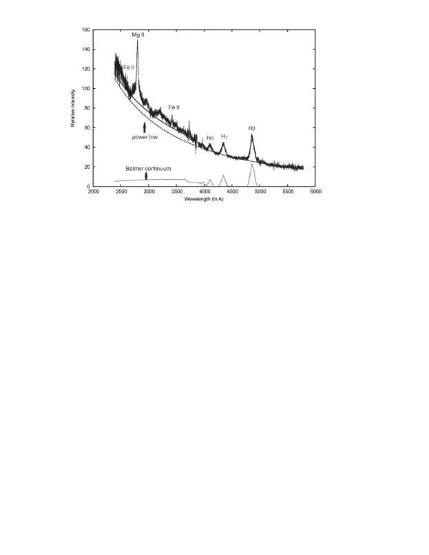
Figure 3: Example of the UV continuum fit (SDSS J092423.42$+$064250.6) with the power law and Balmer continuum model: dotted line - Balmer continuum with high order Balmer lines, dashed lines - power law and solid line - sum of Balmer continuum, high order Balmer lines and power law. The Fe II optical lines, [O III] lines and narrow components of Balmer lines are removed from the spectrum.

To apply the Balmer continuum model, it is important to have a clean profile of strong broad Balmer lines without any contamination from lines that overlap with them (optical Fe II and [O III]), as well as without the narrow component of Balmer lines. We used the fitted data in the optical range to subtract the narrow components and satellite lines, and to obtain the broad Balmer line profile. Then, we applied the same procedure for fitting the UV-pseudocontinuum as described in Kovačević et al. (2014). An example of the UV-pseudocontinuum fit is shown in Fig 3.

Because it is very important to correctly subtract the Balmer continuum in order to measure well the equivalent widths (EWs) of the UV lines, the applicability of the model is tested using the total sample of 293 AGNs chosen for this investigation. We measured the difference between the observed flux and calculated flux (Balmer continuum + power law), and results are presented in Kovačević et al. (2014), Section 3. We found that the discrepancy between the observed and calculated flux in the UV (at $\sim$2650 Å) is smaller than 10% for 92% of the sample. This means that for the majority of the objects from the sample, the EWs are probably measured well. The other 8% of objects, with uncertain continuum determination, do not affect the final result.

2.2.3 The model of the line spectra in the UV ($\lambda\lambda$ 2650-3050 Å) range

After determination and subtraction of the UV-pseudocontinuum, the Mg II 2800 Å line and Fe II template are simultaneously fit.

Note that the Mg II 2800 Å line is the resonant doublet Mg II $\lambda\lambda$ 2795, 2803 Å, where two lines of the doublet cannot be resolved because of their very large widths. The doublet is observed in the spectra of the Type 1 AGNs as a broad, single line. It is very difficult to find an appropriate model to fit the components of the doublet because their relative intensities are not fixed, i.e. their flux ratio depends on optical depth in the line. In general, one can expect a doublet ratio from optically thick gas to be approximately in the range $\lambda$2795/$\lambda$2803$\approx$2:1 to 1:1 (Laor et al., 1997). Additionally, it is not possible to get an unique Gaussian decomposition because two broad Mg II doublet components overlap with central wavelength difference ($\sim\Delta\lambda\approx$ 8 Å). In order to make the fitting procedure more simple, we fit the Mg II doublet as a single Mg II 2800 Å line with two Gaussians: one that fits the core and one that fits the wings of the Mg II 2800 Å  line. In this way, Doppler widths of the Gaussians that fit the core and wings of the single Mg II 2800 Å  line overestimate the Doppler widths of the Mg II doublet components for $\approx$ 260 km s^-1 ($\sim$8 Å separation). Because the widths of the Mg II lines are generally one order of magnitude larger than this value, we assume that it is in the range of the error-bars.

2.2.4 The UV Fe II line emission model

The numerous UV Fe II lines are fitted with the model described in Popović et al. (2003). In this model, the strongest UV Fe II lines, within $\lambda\lambda$ 2650-3050 Å range, are divided into 4 multiplets: 60 ($\lambda\lambda$ 2907-2979 Å), 61 ($\lambda\lambda$ 2861-2917 Å), and additionally with 62 and 63 which overlap at $\lambda\lambda$ 2709-2749 Å. The lines are fitted with 4 parameters of the intensity, for each multiplet. Within one multiplet group, the relative intensities of the lines are fixed using the line strength from NIST (see Popović et al., 2003). It has been assumed that all UV Fe II lines in this range are originating in the same emission region and consequently to have the same Doppler width and shift. Therefore, the UV Fe II template consists of 6 free parameters in the fitting procedure (4 parameters of intensity, width and shift).

The list of the lines and multiplets of the UV Fe II template, as well as the transitions and relative intensities within each multiplet, are given in Table 1. The most intensive line within each multiplet is scaled to the unit intensity.

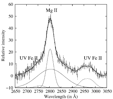
Figure 5: Examples of the fit of Mg II and Fe II lines in the UV range. The best fit is denoted with solid line. The Mg II 2800 line is fitted with two Gaussians: one fitting the core and one the wings. The UV Fe II template is denoted with the dashed line. The flux of the Fe II multiplets 60 and 61 are stronger compared with 62 and 63 for SDSS J095758.44-002354.0 (left) and it is opposite for the object SDSS J155534.61$+$345948.9 (right).

In Fig 4, the multiplet transitions that are included in the template are presented as the Grotrian diagram and shown as a spectrum. The examples of the fitted emission lines (Mg II and UV Fe II) in the UV range are shown in Fig 5. As it can be seen in Fig. 5, there is a significant difference between the intensity of UV Fe II multiplets for different AGN spectra.

2.3 The line parameters

In order to investigate the spectral properties, we obtain the equivalent widths (EWs) of all considered lines and their components. EWs have been measured with respect to the continuum below the lines, after subtraction of all satellite lines. In the case of the UV lines, the intensity of Balmer continuum is estimated first. After that, the Balmer continuum is subtracted and the EWs of the UV lines (Mg II, Fe II UV) are measured with respect to the power law continuum component below the lines.

We measure the Full Width at Half Maximum (FWHM) of broad lines, i.e. Balmer lines (H$\beta$, H$\gamma$ and H$\delta$) and the Mg II line. For the Balmer lines, the FWHM is measured for broad component (ILR + VBLR component), after subtraction of the narrow component. Since Mg II line has no a narrow component, we measure the FWHM for the whole line (Mg II core + Mg II wings). The illustrations of determination of the FWHM for H$\beta$ and Mg II are shown in Fig 6.

3 Results

3.1 Kinematics of the Fe II emission regions

Kinematical properties of the lines (widths and shifts) reflect the motion of the emitting gas. The width of the line (or the line component) depends on random or gravitational bounded motion of the emitting gas, while the shift is caused by the systemic motion of the gas in an emission region. Therefore, similarities between kinematical properties of the different emission lines may indicate a kinematical connection between their emission regions.

In order to investigate the kinematical connections between the UV and optical emission regions, we perform the correlations between the kinematical properties of the analyzed UV and optical emission lines. The widths and shifts of the lines and their components (represented by different Gaussians) are obtained from the best fit. As mentioned in Sec 2.1, in our fitting model we assume that all narrow lines (NLR component of Balmer lines and [O III] lines) are arising in the same emission region, and therefore have the same Doppler widths and shifts.

Similarly, it is assumed that the core components of all Balmer lines arise in ILR, and the wing components in VBLR, and consequently they have the identical kinematical properties. Therefore, we now investigate possible correlations between kinematical parameters of the lines which are the free parameters, i.e. between Balmer components which arise in the NLR, ILR, VBLR, Mg II core, Mg II wings and the Fe II lines in the UV and optical range. The shifts are measured relative to the shift of the narrow lines ([O III] 5007 Å).

The correlations between the line widths and shifts are given in Table 2 and Table 3, and the most significant are shown in Figs 7 and 8. As it can be seen, the strongest kinematical connection is between the UV Fe II, optical Fe II, Mg II core, and Balmer lines core (ILR component).

It is interesting that the correlation between the widths of the UV Fe II and optical Fe II lines is weaker than correlation of their widths with some other lines from the spectral range. The strongest correlation of the UV Fe II width is with the core of the Mg II (r=0.49, P=0; Fig 7, left), whereas its correlations with the widths of the optical Fe II lines and Balmer line ILR component are slightly less significant (r=0.39, P$\approx$2E-12).

The width of the optical Fe II lines has the most significant correlation with the width of the Mg II core as well (r=0.57, P=0; Fig 7, right), and with the Balmer ILR component (r=0.58, P=0; Fig 8, right). The last correlation has was noted in the previous work of Kovačević et al. (2010).

We find that the correlation of the UV Fe II and Fe II optical widths are slightly higher with FWHMs of Mg II and H$\beta$ (core + wings included), than with Mg II core and H$\beta$ ILR components alone (see Table 2). On the other hand, there is no a positive correlation between the iron line widths and the wing component of Mg II or H$\beta$: there is only an anticorrelation with Mg II wings.

The width of Mg II line significantly correlates with the width of Balmer lines. The correlation between FWHM H$\beta$ vs. FWHM Mg II is r=0.77 and P=0 (see Fig. 9). As it can be seen, the objects with $\mathrm{log([OIII]/H\beta}_{NLR}\mathrm{)<0.5}$ (black squares in Fig. 9), are located among the objects with smaller widths of H$\beta$ and Mg II. The Mg II core width correlates with the width of the Balmer line ILR components (r=0.60, P=0; Fig 8, left), while the width of the Mg II wing component decreases as the widths of the Balmer line ILR, UV Fe II, optical Fe II and Mg II core increase (see Table 2). In addition, the wings of the Mg II become narrower when this component is shifted to the red. The H$\beta$ ILR and Mg II core are broader as the H$\beta$ VBLR component is shifted to the red.

Similarly as the widths, the shifts of the optical Fe II, UV Fe II, Mg II core, and H$\beta$ ILR, are correlated (see Table 3) and reflect a kinematical connection between their emission regions. The shifts of the UV and optical Fe II lines have the most significant correlation with the shift of the Mg II core (r=0.48, P=0 for UV Fe II and r=40, P=1.05E-12 for the optical Fe II), whereas the correlations with the H$\beta$ ILR are weaker. The strongest correlation is between the shifts of the Mg II core and Balmer line ILR (r=0.62, P=0).

The relation between the kinematical properties of the optical and UV iron lines is shown in Fig 10. There are only weak trends between their widths, as well as between their shifts.

The average values for widths and shifts of analyzed lines and their components are given in Table 4. It can be seen that the optical and UV Fe II lines have close average values for widths (optical Fe II: 2360 km s^-1, UV Fe II: 2530 km s^-1) with a very large dispersion.

The majority of objects have the Doppler width of the optical Fe II between 1000-3500 km s^-1 and of the UV Fe II between 1500-3000 km s^-1. In Fig 11, the optical and UV Fe II widths are compared with the widths of Balmer line components, which originate from different line emission regions (NLR, ILR, VBLR), and the average values of the widths are assigned. The core of Mg II lines and ILR component of Balmer lines have smaller average Doppler widths (Mg II core: 1590 km s^-1, ILR: 1930 km s^-1). The dispersion of the ILR widths is large as well, and most objects have an ILR width between 1000-3000 km s^-1, whereas the dispersion of the Mg II core is narrower and for 85% of objects the width is within range: 1000-2000 km s^-1. The comparison between the widths of the Balmer line components and Mg II components are shown in Fig 12.

The average shift is significant only for the UV Fe II lines (1150$\pm$580 km s^-1, see Table 4), which seems to be systematically redshifted relative to the narrow lines. All other analyzed lines (optical Fe II, Mg II and H$\beta$ components) have no significant average velocity shift.

3.2 Correlations between the UV and optical emission line parameters

A line EW reflects the emission line strength relative to the total continuum and it depends on a number of physical parameters of the emitting plasma, such as, e.g. electron density, temperature, the strength of the photoionizing flux, optical depth for the line, etc. We measure the EWs of broad and narrow lines from the spectral range and we find their averaged values for the sample, and for two subsamples with $\mathrm{log([OIII]/H\beta}_{NLR}\mathrm{)<0.5}$ (SB dominant) and $\mathrm{log([OIII]/H\beta}_{NLR}\mathrm{)>0.5}$ (AGN dominant). The results are shown in Table 5. As it can be seen, there are differences between AGN and SB dominant objects, and the biggest one is for the average EW of the optical Fe II and [O III] lines. The SB dominate subsample has significantly higher EW of optical Fe II and weaker EW [O III] than the AGN dominant subsample.

We explore the correlations between the EWs of the optical and UV lines and their components (see Table 6). We can summarize the correlations given in Table 6 as: (i) there is no any correlation between the EWs of the optical and UV Fe II lines; (ii) the EW Fe II UV correlates only with the EW Mg II_total; (iii) the EW Fe II optical shows only anticorrelation with EW [O III] (Boroson & Green, 1992; Kovačević et al., 2010); (iv) the EW [O III] correlates with EWs of all analyzed lines and line components (broad and narrow), except with the EW Fe II UV and anticorrelates only with the EW Fe II optical; (v) there is a correlation among EWs of all narrow lines; (vi) the EW Mg II correlates with EWs of all analyzed broad lines except with EW Fe II optical.

There is no correlation between the EWs of the optical and UV Fe II lines. The plot between the optical Fe II and multiplet 60 of the UV Fe II is shown in Fig 13. The multiplet 60 of the UV Fe II was chosen because it is well defined feature at $\sim$2950 Å and it does not overlap with extended Mg II wings. It can be seen that objects with a dominant starburst radiation (black squares in Fig 13) generally have a strong optical Fe II emission, while such trend cannot be seen for the UV Fe II lines.

The correlations between the widths and EWs of the considered emission lines are shown in Table 7. The most interesting correlations in this table are those with the EW of the optical Fe II and the line widths. While EWs of the Fe II_UV60, H$\beta$ NLR and Mg II line increase, their line widths increase as well; however, the opposite happens for the EW of the optical Fe II lines: the EW Fe II optical increases as its width decreases. Moreover, EW Fe II_optical anticorrelates with the widths of all analyzed broad lines, especially with FWHM H$\beta$ and FWHM Mg II (see Fig 14). The objects with dominant SB emission (black squares in Fig. 14), as expected, have a strong optical Fe II emission and narrower H$\beta_{broad}$ and Mg II lines.

3.2.1 The flux ratios of the emission lines

We explore the correlations between the line properties and flux ratios $\mathrm{FeII}_{opt}/\mathrm{FeII}_{UV60}$, $\mathrm{FeII}_{opt}/\mathrm{MgII}$, $\mathrm{FeII}_{UV}/\mathrm{MgII}$, $\mathrm{MgII}/\mathrm{H\beta_{broad}}$, $\mathrm{[OIII]_{5007}}/\mathrm{H\beta_{NLR}}$, $\mathrm{H\beta}_{broad}/\mathrm{H\gamma}_{broad}$ (see Table 8). These flux ratios are chosen because they may be indicators of some physical conditions or the abundance in the emission line regions.

Different models of the iron emission predict that the ratio of $\mathrm{FeII}_{opt}/\mathrm{FeII}_{UV}$ could be an indicator of the column density, due the atomic properties of the iron ion (see Joly, 1987; Sameshima et al., 2011). Verner et al. (2003) and Sameshima et al. (2011) found that this ratio depends on microturbulence, i.e. the increase of the $\mathrm{FeII}_{opt}/\mathrm{FeII}_{UV}$ ratio reflects the increase of the column density and the decrease of the microturbulence in the emitting gas. It has been found that this ratio anticorrelates with FWHM Mg II (Tsuzuki et al., 2006) and FWHM H$\beta$ (Dong et al., 2011), but correlates with the Eddington ratio (Sameshima et al., 2011; Dong et al., 2011).

Table 8 shows several correlations between this ratio and the different line properties. We found that the ratio $\mathrm{FeII}_{opt}/\mathrm{FeII}_{UV60}$ increases as: (i) the widths of all analyzed broad lines decrease (H$\beta$, Mg II, optical and UV Fe II); (ii) the EW Mg II decreases.

The correlations between the $\mathrm{FeII}_{opt}/\mathrm{FeII}_{UV60}$ ratio and FWHMs of H$\beta$ and Mg II are presented in Fig 15. Note that SB dominant objects (assigned with black squares) are in the upper part of graphs among the objects with a high $\mathrm{FeII}_{opt}/\mathrm{FeII}_{UV60}$ ratio and small FWHM H$\beta$ and FWHM Mg II widths.

The ratio $\mathrm{FeII}/\mathrm{MgII}$ is considered by several authors to be a cosmological abundance indicator (Hamman & Ferland, 1993; Matteucci & Recchi, 2001; Verner et al., 2003; Dong et al., 2011; De Rosa et al., 2011). Until now, no relation has been found between this ratio and cosmological redshift, which may be a consequence of the additional influence of the physics of the emission region to this ratio. The model of Verner et al. (2003) predicts that the $\mathrm{FeII}_{UV}/\mathrm{MgII}$ ratio is sensitive on microturbulence. Similar to the $\mathrm{FeII}_{opt}/\mathrm{FeII}_{UV60}$ ratio, the $\mathrm{FeII}_{opt}/\mathrm{MgII}$ increases as the FWHM Mg II and FWHM H$\beta$ decrease (Tsuzuki et al., 2006; Dong et al., 2011), and Eddington ratio increases (Dong et al., 2011).

In our sample we analyze the both ratios, $\mathrm{FeII}_{opt}/\mathrm{MgII}$ and $\mathrm{FeII}_{UV}/\mathrm{MgII}$, and we find that correlations with some spectral properties are different for these two ratios. The $\mathrm{FeII}_{opt}/\mathrm{MgII}$ ratio increases as the widths of the broad lines (except Fe II UV) decrease, while the ratio $\mathrm{FeII}_{UV}/\mathrm{MgII}$ does not correlate with these properties. Both ratios ($\mathrm{FeII}_{opt}/\mathrm{MgII}$ and $\mathrm{FeII}_{UV}/\mathrm{MgII}$) anticorrelate with EW [O III] and EW H$\beta_{broad}$. The correlation of the $\mathrm{FeII}_{opt}/\mathrm{MgII}$ and the widths of H$\beta_{broad}$ and Mg II are presented in Fig 16. The starburst dominant objects (black squares in Fig 16) have a high ratio of $\mathrm{FeII}_{opt}/\mathrm{MgII}$.

The ratio $\mathrm{MgII}/\mathrm{H\beta_{broad}}$ may be taken as an indicator of the element abundance in AGNs. This ratio correlates with the width of the Mg II and with EW $\mathrm{FeII}_{UV}$, that shows how beside the abundance, other effects can affect on the $\mathrm{MgII}/\mathrm{H\beta_{broad}}$ ratio.

Finally, the ratio $\mathrm{[OIII]_{5007}}/\mathrm{H\beta_{NLR}}$ is assumed to be an indicator of the starburst activity. Namely, the ratios of some narrow lines reflect the shape of ionizing continuum, i.e. whether the ionization source is the accretion disc around black hole or hot, young stars. This fact is used in the construction of the diagnostic diagrams based on the narrow line ratios (see Baldwin, Phillips & Terlevich, 1981; Veilleux & Osterbrock, 1987). Popović & Kovačević (2011) found that the $\mathrm{[OIII]}/\mathrm{H\beta_{NLR}}$ ratio (which is usually used as one axis in diagnostic diagrams) could be used as an approximate indicator of the presence or absence of the starburst activity in AGN spectra.

We analyze the correlations between this ratio and other spectral properties in our sample (see Table 8), and find that as $\mathrm{[OIII]}/\mathrm{H\beta_{NLR}}$ ratio increases (which indicate smaller contribution of SB fraction): (i) the narrow lines become narrower; (ii) the broad lines become broader; (iii) the EWs of [O III], H$\beta_{broad}$ and Mg II increase; (iv) the EW of Fe II_opt decreases.

On the other hand, the objects that may have significant SB activity near an AGN (which is reflected as decrease of this ratio), have a smaller difference in the width of the narrow and broad lines, stronger Fe II_opt lines, and weaker [O III], H$\beta_{broad}$ and Mg II. No correlation is seen for the EW of Fe II_uv.

It is found that the ratio of the broad Balmer lines may be an indicator of the intrinsic dust extinction (Dong et al., 2008). However, this should not strongly affect the ratio $\mathrm{H\beta}_{broad}/\mathrm{H\gamma}_{broad}$ because the extinction effects on the lines are similar (close transition wavelengths). Under some circumstances this ratio can be used for the diagnostic of the physical parameters in the BLR plasma (see, e.g. Popović, 2003; Ilić et al., 2012). We found that the $\mathrm{H\beta}_{broad}/\mathrm{H\gamma}_{broad}$ ratio increases as: (i) the FWHM H$\beta$, FWHM Mg II and the Fe II_opt width increase (see Table 8); (ii) the EW Fe II_opt decreases (r= - 0.49, P=0, Fig 17) and EW [O III] increases (r= 0.34, P=1.3E-9). The correlation with line widths may indicate some connections between the kinematics and physics of the emitting gas. Fig 17 shows that objects with strong starburst activity (black squares) have large values of the Fe II optical, and the smallest values of the $\mathrm{H\beta}_{broad}/\mathrm{H\gamma}_{broad}$ ratio.

Some of these ratios correlate between each other. For example, as $\mathrm{[OIII]}/\mathrm{H\beta_{NLR}}$ increases, $\mathrm{H\beta}_{broad}/\mathrm{H\gamma}_{broad}$ increases as well, but $\mathrm{FeII}_{opt}/\mathrm{FeII}_{UV60}$ and $\mathrm{FeII}_{opt}/\mathrm{MgII}$ decrease. The ratio $\mathrm{H\beta}_{broad}/\mathrm{H\gamma}_{broad}$ anticorrelates with $\mathrm{FeII}_{opt}/\mathrm{MgII}$ and $\mathrm{FeII}_{UV}/\mathrm{MgII}$, and $\mathrm{MgII}/\mathrm{H\beta_{broad}}$ anticorrelates with $\mathrm{FeII}_{opt}/\mathrm{FeII}_{UV60}$.

Note that the width of the narrow Balmer line component and the width of the broad Balmer component have opposite trends with the some ratios, especially with $\mathrm{[OIII]}/\mathrm{H\beta_{NLR}}$ (see Table 8). Also, the EWs of the optical Fe II and [O III] have opposite correlations with all considered ratios ($\mathrm{FeII}_{opt}/\mathrm{FeII}_{UV60}$, $\mathrm{FeII}_{opt}/\mathrm{MgII}$, $\mathrm{FeII}_{UV}/\mathrm{MgII}$, $\mathrm{H\beta}_{broad}/\mathrm{H\gamma}_{broad}$ and $\mathrm{OIII}/\mathrm{H\beta_{NLR}}$), except with $\mathrm{MgII}/\mathrm{H\beta_{broad}}$. This reflects the EW Fe II vs. EW [O III] anticorrelation.

The averaged flux ratios of emission lines are given in Table 9. As it can be seen, the optical Fe II lines (in range 4400-5500 Å) are, on average, about five times stronger than the UV ones (in range 2900-2980 Å, multiplet 60), whereas in the SB dominant subsample they are $\sim$7.5 times stronger than the UV ones. It is interesting that the ratio of $\mathrm{FeII}_{opt}/\mathrm{MgII}$ (which is expected to be a cosmological indicator) is significantly higher in the SB dominant subsample ($\sim$1.4) compared with the AGN dominant subsample ($\sim$0.8).

4 Discussion

4.1 Location of the UV Fe II emitting region

In our previous work, we discussed the location of the optical Fe II emission region (see Popović et al., 2009; Kovačević et al., 2010; Shapovalova et al., 2012), and found that it is located in an outer part of the BLR (so-called the ILR), which is recently confirmed by Fe II reverberation (see Barth et al., 2013).

The correlation between the widths of the optical Fe II and UV Fe II lines indicates that the UV Fe II emission region is probably located close to the Fe II optical one. Moreover, the widths and the shifts of the UV and optical Fe II lines are correlated with the widths and shifts of the Mg II core and H$\beta$ ILR component (see Table 2 and Table 3). The average widths of the UV and optical Fe II lines are very similar (2530 km s^-1 and 2360 km s^-1), and they are both broader than the average widths of the H$\beta$ and Mg II cores (1930 km s^-1 and 1590 km s^-1). The correlation of the iron lines width is even more significant with the FWHM of the total broad profile (wings + core) of Mg II and H$\beta$, but there is no a positive correlation with the separated wing component of these lines. It seems that the iron lines (both, UV and optical) generally originate in the outer part of the BLR (ILR). However, as we mentioned in Kovačević et al. (2010), there may be an additional emission of the Fe II lines (in the UV and optical) that is coming from the inner part of BLR (VBLR). This emission is probably contributing to the continuum because the lines are very broad and cannot be resolved in the bulk of Fe II lines in the UV and optical spectral ranges.

In order to test the location of the forming region of the UV and optical Fe II lines, we searched for the same geometry as in the Mg II and H$\beta$ emission regions. We modified the UV and optical iron templates, assuming that the profiles of the iron lines are the same as the profiles of the Mg II or H$\beta$. We compared the accuracy of the new fits with the previous, single Gaussian model (see Appendix A). We found that: (a) Single Gaussian profile gives better fit for the UV iron lines, compared with Mg II and H$\beta$ profiles, (b) H$\beta$ profile fits slightly better optical Fe II than single Gaussian profile. This indicates that, at least in the optical Fe II lines, there is a contribution of the VBLR emission.

The averaged values of line widths are similar for the UV and optical Fe II. However, there is a great difference in the the averaged values of their shifts. For the optical Fe II the shift is 350$\pm$510 km s^-1, whereas for the UV Fe II is much larger: 1150$\pm$580 km s^-1. Therefore, the systemic redshift (relative to the [O III]) could be significantly detected only in the UV Fe II, but it is not significant in the optical Fe II.

The absence of the significant redshift found for the optical Fe II is in the agreement with the previously obtained result: 100$\pm$240 km s^-1 (Kovačević et al., 2010). Sulentic et al. (2012) could not confirm redshift in the optical Fe II lines, as well, but Hu et al. (2008a) found a slight redshift in the optical Fe II: 407$\pm$200 km s^-1. Note that between the shifts of the optical and UV Fe II there is no a significant correlation, but only a weak trend.

We should note here that the large averaged redshift of the UV Fe II should be taken with the caution, because of uncertainties in the fit of the UV Fe II in some spectra. The UV Fe II lines can be very broad, which makes it difficult to resolve them from the Mg II wings.

The systemic redshift probably represents the infall of the emitting gas (Hu et al., 2008a; Ferland et al., 2009). Hu et al. (2008a) found the correlation between the optical Fe II systemic redshift and L${}_{bol}/$L_Edd, and they speculate that the inflow is driven by gravity toward the center and decelerated by the radiation pressure. Ferland et al. (2009) investigated the geometry of the Fe II emission region, taking into account the distribution of emitting clouds. If the distribution of emitting clouds is symmetric, we see the same number of clouds from their illuminated as from their shielded faces. But if distribution of emitters is asymmetric, we mainly observe Fe II emission from the shielded face of infalling clouds, which is reflected in the systemic redshift of the Fe II lines (Ferland et al., 2009). Their calculation show that the distribution of the UV Fe II emission region is more asymmetric than the distribution of the optical Fe II. This model reproduces well the observed $\mathrm{FeII}_{opt}/\mathrm{FeII}_{UV}$ flux ratio.

The results from this paper, the significant average systemic redshift for the UV Fe II, and absence of the significant redshift for the optical Fe II, support the model given by Ferland et al. (2009). Although the UV and optical Fe II emission is emitted from approximately the same region in the AGN structure, it might be that the distribution of emitting clouds is different: the UV Fe II emission clouds are probably distributed asymmetrically, while the optical Fe II ones have the isotropic distribution.

Other explanations of the results, except asymmetry of the emission region, are also possible. One can speculate that an inflow can be associated with internal shock waves, which may contribute to more effective excitation of the UV lines (see Dopita & Sutherland, 2005). Namely, it is possible that UV Fe II lines are more excited in infalling gas, compared with the optical Fe II. For example, some connection between Mg II flux and jet emission is detected in León-Tavares et al. (2013).

4.2 Peculiarities of the optical Fe II correlations

Concerning correlations between the optical Fe II lines and analyzed UV/optical lines, we can point out several peculiarities:

1. Only the EW of the optical Fe II anticorrelates with the EW of some other line (EW [O III]), while all other lines correlate with EWs of other lines or show no correlations (Table 6). This specific anticorrelation is reflected through correlations shown in Table 8, as well, where the EW Fe II and EW [O III] have opposite correlations with considered ratios.

2. The EWs of analyzed lines (UV Fe II, H$\beta$ NLR and Mg II) increase as their widths increase, or there is no any correlation between their EWs and widths as for H$\beta_{broad}$ and [O III] (Table 7). Only in the case of the optical Fe II, their EW increases as the width decreases, i.e. the Fe II lines are stronger as they are narrower. In addition, while EWs of the broad lines do not depend on widths of the other lines, the EW of the optical Fe II becomes stronger as other broad lines are narrower (Mg II, H$\beta$). It is interesting that it is the same with the EW H$\beta$ NLR, which increases as the width of the broad lines decreases.

On the other hand, the UV Fe II lines do not show any of these peculiar correlations as the optical Fe II, e.i. it seems that their emission properties are quite different than for the optical Fe II.

4.3 Differences between the UV and optical Fe II lines

As it can be seen in previous sections, there are significant differences between the optical and UV Fe II lines, as reflected in different correlations of these lines with the other spectral properties. Between the EWs of these lines there is no correlation (see Sec 3.2), and their flux ratio depends on different physical parameters, such as column density and microturbulence (see Joly, 1987; Verner et al., 2003, 2004; Sameshima et al., 2011). These differences could be explained in two ways: the emission regions of optical and UV Fe II lines have a different spacial distribution, or the mechanisms of their excitation are not the same. The mixture of these two influences is also possible.

Joly (1987) suggested as one of the solutions that the optical and UV Fe II could be emitted in two distinct regions. Ferland et al. (2009) concluded that iron lines are emitted by clouds that are distributed asymmetrically: the UV Fe II lines are beamed toward a central source while the optical Fe II lines are emitted isotropically. In the case of asymmetrical distribution, photoionization models can reproduce the observed UV to optical Fe II flux ratio (Sameshima et al., 2011). Our analysis of the kinematical properties of the optical and UV Fe II lines indicates that their emission regions are located close to one another in the AGN structure. Also, unlike optical Fe II emission region, the UV Fe II emission region is probably asymmetric. Different distributions of the iron emission clouds in an emission region can explain their observed flux ratios, but it still cannot explain the peculiar correlations of the optical Fe II lines with some line properties, which is not detected for the UV Fe II.

It is possible that UV and optical Fe II arise with the domination of different excitation mechanisms, which could explain their differences. Joly (1987) found that strong optical Fe II emitters can be explained with the collisional excitation in a dense and cold medium (6000 K $<$ T $<$ 8000 K, n${}_{H}>10^{11}$ cm^-3), while Fe II UV intensities are more difficult to account for. The models of Joly (1987) show that optical and UV Fe II have different correlations with the column density, due the larger optical depth of the UV Fe II lines. For N${}_{H}>$ 21 cm^-2, the optical Fe II lines increase more rapidly than the UV Fe II ones, because of a smaller optical thickness. For a larger column density (N${}_{H}>$ 22 cm^-2), the UV Fe II flux decreases more rapidly than the flux of the optical Fe II (see Joly, 1987). It is the reason why the flux ratio of $\mathrm{FeII}_{opt}/\mathrm{FeII}_{UV}$ increases with increasing of the column density.

Sameshima et al. (2011) found that $\mathrm{FeII}_{opt}/\mathrm{FeII}_{UV}$ ratio increases with increasing of the Eddington ratio. A high Eddington ratio is related to dense medium and large column density, because the clouds with a low density and small column density would be blown away by a large radiative pressure (Dong et al., 2009, 2011).

On the other hand, the large column density and the dense environment may be also due to an increase of the star formation rate (Netzer et al., 2004; Harris et al., 2013; Clowes et al., 2013). Netzer et al. (2004) found that a violent starforming activity can produce high-density and large column density gas in nuclear regions.

The presence of starforming/starburst regions could be related with AGN evolution (Mao et al., 2009; Sani et al., 2010). The spectral properties of AGNs are probably changing during the time, and it is expected that young AGNs have a higher Eddington ratio, higher star formation rate, and smaller black hole mass and FWHMs of the broad lines (Lípari & Terlevich, 2006; Sani et al., 2010).

Since the objects in this sample have a redshift in range 0.407$<$z$<$0.643, we cannot explore evolution at high redshift, but we cannot exclude that objects with similar z could be in different evolution phase. This may explain some correlations that are typical for the optical Fe II lines found in this paper (see Sec. 4.2), as well as correlations which are part of Boroson and Green Eigenvectror 1 (Boroson & Green, 1992): EW Fe II optical vs. EW [O III] and EW Fe II optical vs. FWHM H$\beta$. The anticorrelation of the optical Fe II and [O III] equivalent widths could be caused by an increase in density and the column density due to the influence of the starbursts: as the column density increases, the flux of the optical Fe II increases, but the flux of the forbidden [O III] lines decreases, because of the collisional suppression or the weak ionizing continuum from starbursts. This anticorrelation is not seen for EWs of the UV Fe II and [O III], because the UV Fe II lines decrease more rapidly with increasing column density, compared with the optical Fe II (Joly, 1987). Sameshima et al. (2011) suggested that increasing column density, caused by a large Eddington ratio, is a physical cause behind the Boroson and Green Eigenvectror 1 correlations, but they explain the decrease of the [O III] lines as inability of ionizing photons emitted from the central object to reach the NLR clouds, because the large-column-density clouds in the BLR. In this case, we would expect the anticorrelation between the EWs of the optical Fe II and other narrow emission lines (e.g. narrow component of H$\beta$), but these correlations are not observed (see Kovačević, 2011). The pure recombination lines, as the NLR H$\beta$, are not influenced by higher densities, while forbidden [O III] lines would be weaker in a dense medium because of the collisional suppression. Also, unlike the [O III] lines, the Balmer lines are strongly ionized by starburst continuum.

Sani et al. (2010) investigated a sample of the AGNs from the local Universe (z $<$ 0.2) using the Spitzer data and found that star formation rate is higher in objects with low FWHMs of the broad lines, low black hole mass and high Eddington ratio. Also, in model of Lípari & Terlevich (2006) young AGNs are expected to have the FWHM of the broad lines smaller than the older ones, because the BLR is not developed yet. This may explain other correlations typical for the optical Fe II, as e.g. an anticorrelation EW Fe II optical vs. FWHM H$\beta$. The Fe II optical emission is stronger in a high density/large column density environment, which is expected in young objects with the high Eddington ratio, high star formation rate and relatively narrower broad emission lines. In our sample, we also find an anticorrelation between the EW Fe II optical and the widths of the Fe II optical and Mg II.

If we assume that the ratio $\mathrm{[OIII]}/\mathrm{H\beta_{NLR}}$ is an indicator of the starburst fraction (the increasing ratio reflects the decreasing starburst influence), than the found correlations of this ratio with the other spectral properties supports this model. In Table 8 and Figs 9, 13, 14, 15, 16 and 17 it could be seen that for the strong starbust influence (small values of the $\mathrm{[OIII]}/\mathrm{H\beta_{NLR}}$ ratio), the broad lines are narrower, the narrow lines are broader, EW of the optical Fe II is stronger and the EW of the [O III] is weaker. In difference with the optical Fe II, the EW of UV Fe II does not depend on the starburst influence (see Table 8 and Fig 13). Also the anticorrelation of this ratio with the ratios $\mathrm{FeII}_{opt}/\mathrm{FeII}_{UV60}$ and $\mathrm{FeII}_{opt}/\mathrm{MgII}$, which depend on the column density and microturbulence, imply that for starburst dominant objects, the column density is larger and microturbulence is smaller, compared with the gas in pure AGNs.

A high density may stimulate some excitation processes that have a more important role for the optical Fe II. This could be the collisional excitation or increased Ly$\alpha$ fluorescence, which may be one of the very important additional mechanisms of the Fe II excitation (Penston, 1987; Graham et al., 1996; Sigut and Pradhan, 1998; Bautista et al., 2004).

The model we have is discussed here certainly is not an unique interpretation of the data. We may speculate about some other explanations of these correlations. For example, they could be consequence of the different viewing angle. It is possible that visibility of the optical Fe II emission region increases as we get a more pole-on view of the BLR, while the broad line widths decrease. This could be reflected as an anticorrelation of the optical Fe II strength and broad line width. There are some indications that EW [O III] also depends on inclination (see Risaliti et al., 2011), which can be the explanation for the anticorrelation of the optical Fe II lines and [O III]. In this case, these anticorrelations are not seen for the UV Fe II lines because their emission region has the different spacial distribution than the optical Fe II one.

5 Conclusions

In this paper we investigate the connections between the UV and optical Fe II emission lines using a sample of the 293 AGNs from the SDSS database. The properties of the optical and UV iron lines are compared and correlated with the properties of the other emission lines that are present in the observed spectral range, in order to investigate the origin of the iron lines and processes responsible for their emission. We model the UV Fe II emission taking into account the contribution of the different multiplets (Popović et al., 2003). Additionally, we use a new model for the Balmer continuum subtraction (Kovačević et al., 2014). The strong emission lines are decomposed into components that are coming from the different emission regions, in order to explore and compare the physical properties of the environment where the components arise. The flux ratios of the lines, which can be the indicators of the physical conditions in the emission region, are also analyzed. We consider the influence of starburst activity to the spectral properties of the iron emission. After investigation of correlations between the UV/optical Fe II and other lines from the spectral range, we can outline the following conclusions:

1. The UV and optical Fe II lines arise in the close emission regions in the AGN structure. Most of the Fe II UV/optical emission is probably originating in the Intermediate Line emission Region i.e. a region with Doppler velocities around 1500-2000 $\rm kms^{-1}$. However, the Fe II lines tend to be broader than the ILR components of H$\beta$ and Mg II, which indicates a small contribution of VBLR emission, at least in the Fe II optical lines.

2. The significant systemic redshift, which is the signature of the gas infall, is found only for the UV Fe II lines (1150$\pm$580 km s^-1), but not for the optical Fe II (350$\pm$510 km s^-1). This indicates that, although the UV and optical Fe II emission clouds are located in approximately the same region of the AGN structure, their distribution is probably different: the UV Fe II emission clouds seem to be distributed asymmetrically (we see more shielded, infalling clouds) while the optical Fe II emission clouds are probably isotropically distributed. Except emission region asymmetry, some other models can explain high UV Fe II redshift, e.g. more efficient excitation of the UV Fe II lines in the infalling gas, due to shock waves.

3. There are significant differences between the optical and UV Fe II lines, which are presented in different correlations between these lines and other spectral properties. The intriguing anticorrelations found for the optical Fe II (EW Fe II_opt vs. EW [O III] and EW Fe II_opt vs. FWHM H$\beta$), which are part of the Boroson & Green (1992) Eigenvector 1, are not detected for the UV Fe II. Beside all analyzed broad lines, only the EW Fe II_opt anticorrelates with EW some other emission line ([O III]), and only EW Fe II_opt increases as the widths of all broad lines (including Fe II_opt) decrease.

4. The peculiar anticorrelations of the optical Fe II are probably connected with a high density and a large column density region in AGNs with a high star formation rate. The anticorrelation between EWs of the optical Fe II and [O III] lines is probably due increase of the additional excitation mechanism of the optical Fe II with the increase of the column density, and at the same time, a decrease of the forbidden [O III] lines due collisional suppression, or because of low ionization continuum from starbursts. On the other hand, the anticorrelation EW Fe II_opt vs. FWHM H$\beta$ is present because the AGNs, with high star formation rate and large column density regions, are expected to be young objects with a smaller mass of the black hole and widths of the broad lines that are generally narrower than in the spectra of older, pure AGNs. These correlations are not detected in the UV Fe II lines, since their optical thickness is larger than for optical Fe II, so with increasing column density, UV Fe II lines decrease more rapidly than optical Fe II. Other explanations of the these correlations are possible. For example, they could be caused by different angle of view.

Additionally, we explore some correlations between the Mg II and Balmer lines, as well as between the flux ratio of different lines and kinematical parameters. From this investigation we can outline following conclusions:

1. There is an expected good correlation between FWHMs of the broad Mg II and H$\beta$ line. Both, the Mg II and broad Balmer lines can be decomposed into two components, the VBLR and ILR, which shows a complex structure of the BLR. Moreover, there is an anticorrelation between the width and shift of the Mg II wing component, that indicates the asymmetry in the Mg II, i.e. the narrower Mg II wing component tends to be asymmetric.

2. It seems that the explored line ratios (see Table 8) are connected with the FWHMs of broad lines, especially with FWHM Mg II, where a positive trend between FWHM Mg II and ratios $\mathrm{H\beta}_{broad}/\mathrm{H\gamma}_{broad}$ and $\mathrm{MgII}/\mathrm{H\beta_{broad}}$ is found, and anticorrelations with $\mathrm{FeII}_{opt}/\mathrm{FeII}_{UV60}$ and $\mathrm{FeII}_{opt}/\mathrm{MgII}$. This is an indicator that the physical processes and abundances in the BLR, which are reflected in the ratios, are connected with the emission region kinematics.

Appendix A The fitting of the iron lines with Mg II and H$\beta$ profiles

In order to fit the optical iron lines with the H$\beta$ line profile, we modify the iron template, so that instead of one Gaussian for each iron line, there are two Gaussians with the same widths, relative shifts, and relative intensities as the ILR and VBLR H$\beta$ components. We keep the same relative intensities between the iron lines in the multiplets as in the initial, single Gaussian template, and the shift of the template is the free parameter. We fit simultaneously the H$\beta$ line and the optical Fe II template made of the sum of H$\beta$ profiles. After that, we applied the other template made of the Mg II profiles, where the widths, relative shifts, and relative intensities of the Mg II core and the wings are fixed values obtained from the fit in the UV part of spectrum. We repeat this procedure for the UV Fe II lines using Mg II and H$\beta$ profiles in the UV Fe II template in the same way, but this time Mg II line is fitted simultaneously with UV Fe II template, which is made of Mg II profiles. For template with H$\beta$ profiles we use the fixed values of H$\beta$ parameters, which were obtained from the fit in the optical range. An example of the one object fit (SDSS J020435.18$-$093154.9) with the different iron templates is given in Figs 18 and 19. It can be seen that fit of the optical Fe II lines with H$\beta$ profiles (B) is slightly better than with single Gaussian model (A), whereas the iron template with Mg II profiles cannot fit well the optical iron lines (C). In the case of the UV Fe II lines, the single Gaussian model (A) fits the iron lines better, than other two templates (B and C).

We compare the $\chi^{2}$ of the fits obtained from the different templates with the $\chi^{2}$ of the initial fit where the iron lines are fitted with one Gaussian for each line. The results for the whole sample are given in Table 10. Generally, the differences between $\chi^{2}$ obtained with different templates are, for most of objects, small and less than 5%. The fit of the optical iron lines with the H$\beta$ profiles gives a slightly better fit, comparing the single Gaussian model for $\sim$85 % of objects from the sample. Only in 3% of objects, fit is significantly improved (the difference between $\chi^{2}$ higher than 10%). In the case of the fit of optical iron lines with the Mg II profile, only in the half of the sample fits are better. The fit of the UV iron lines is less accurate with H$\beta$ and Mg II profiles than with one Gaussian model for the majority of objects from the sample.

Figure 1: Distribution of the redshift (left) and luminosity (right) in the sample of 293 AGNs.

Figure 2: Example of the fit of spectrum of SDSS J020039.15$-$084554.9 in the $\lambda\lambda$ 4000-5500 Å region. A: The observed spectrum (dots) and the best fit (solid line). B: Decomposition of the emission lines. Fe II template is denoted with dashed line. C: The Fe II template is shown separately.

Figure 4: Strongest Fe II multiplets within the $\lambda\lambda$ 2650-3050 Å wavelength range are shown in the Grotrian diagram (top) and in the spectrum (middle). The total UV Fe II template is shown in the bottom. In this example, the intensity ratio for multiplets 60, 61, 62, 63 is taken to be: 10:5:0.03:0.07, respectively.

Figure 6: Example of measuring FWHM of H$\beta$ (left) and Mg II (right).

Figure 7: Correlation between the Doppler widths of Mg II 2800 core and UV Fe II (left) and optical Fe II (right).

Figure 8: Correlation between Doppler widths of the Balmer line ILR component and Mg II 2800 core (left) and Fe II optical (right).

Figure 9: Correlation between the FWHMs of Mg II and H$\beta$. The fit with linear function f(x)=A*x+B, gives the values: A=0.504$\pm$0.026 and B=1086.09$\pm$135.2. Black squares: the objects with $\mathrm{log([OIII]/H\beta}_{NLR}\mathrm{)<0.5}$ (with dominant starburst radiation), x-marks: the objects with $\mathrm{log([OIII]/H\beta}_{NLR}\mathrm{)>0.5}$ (pure AGNs).

Figure 10: Trend between the Doppler widths (left) and velocity shifts (right) of the optical and UV iron lines.

Figure 11: Comparison between the widths of the Balmer line components and the widths of optical (left) and UV (right) Fe II lines. The widths of the Balmer line components are presented on Y-axis as: NLR (white squares), ILR (black squares) and VBLR (circles). The average values of widths are assigned with dotted line.

Figure 12: Same as in previous Figure, just for the widths of Mg II core (left) and Mg II wings (right).

Figure 13: Correlation between the EWs of optical and UV Fe II. Black squares: the objects with $\mathrm{log([OIII]/H\beta}_{NLR}\mathrm{)<0.5}$, x-marks: the objects with $\mathrm{log([OIII]/H\beta}_{NLR}\mathrm{)>0.5}$.

Figure 14: Correlations between EW of optical Fe II and FWHM of the broad H$\beta$ (left) and FWHM of Mg II (right). Black squares: the objects with $\mathrm{log([OIII]/H\beta}_{NLR}\mathrm{)<0.5}$, x-marks: the objects with $\mathrm{log([OIII]/H\beta}_{NLR}\mathrm{)>0.5}$.

Figure 15: Correlations between the $\mathrm{FeII}_{opt}/\mathrm{FeII}_{UV60}$ and FWHM H$\beta$ (left) and Mg II width (right). Black squares: the objects with $\mathrm{log([OIII]/H\beta}_{NLR}\mathrm{)<0.5}$, x-marks: the objects with $\mathrm{log([OIII]/H\beta}_{NLR}\mathrm{)>0.5}$.

Figure 16: Same but for the $\mathrm{FeII}_{opt}/\mathrm{MgII}$ ratio. Black squares: the objects with $\mathrm{log([OIII]/H\beta}_{NLR}\mathrm{)<0.5}$, x-marks: the objects with $\mathrm{log([OIII]/H\beta}_{NLR}\mathrm{)>0.5}$.

Figure 17: Correlation between $\frac{H\beta}{H\gamma}$ and the EW of optical Fe II. Black squares: the objects with $\mathrm{log([OIII]/H\beta}_{NLR}\mathrm{)<0.5}$, x-marks: the objects with $\mathrm{log([OIII]/H\beta}_{NLR}\mathrm{)>0.5}$.

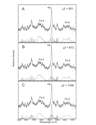
Figure 18: Example of the fit of the optical iron lines with single Gaussian model (A), with H$\beta$ profile (B) and Mg II profile (C), for object: SDSS J020435.18$-$093154.9. The iron template is denoted with dashed line.

Figure 19: Same as in previous figure, but for the UV iron lines.

Table 1: The list of the strongest UV Fe II lines within $\lambda\lambda$ 2650-3050 Å range used in model.

Wavelength	Multiplet	Transitions	Relative intensity
2926.58	60	a${\ }^{4}D_{7/2}$ - z${\ }^{6}F^{o}_{9/2}$	1.000
2953.77	60	a${\ }^{4}D_{5/2}$ - z${\ }^{6}F^{o}_{7/2}$	0.842
2970.51	60	a${\ }^{4}D_{3/2}$ - z${\ }^{6}F^{o}_{5/2}$	0.386
2979.35	60	a${\ }^{4}D_{1/2}$ - z${\ }^{6}F^{o}_{3/2}$	0.165
2916.15	60	a${\ }^{4}D_{7/2}$ - z${\ }^{6}F^{o}_{7/2}$	0.007
2945.26	60	a${\ }^{4}D_{5/2}$ - z${\ }^{6}F^{o}_{5/2}$	0.007
2975.94	60	a${\ }^{4}D_{1/2}$ - z${\ }^{6}F^{o}_{1/2}$	0.039
2907.85	60	a${\ }^{4}D_{7/2}$ - z${\ }^{6}F^{o}_{5/2}$	0.015
2939.51	60	a${\ }^{4}D_{5/2}$ - z${\ }^{6}F^{o}_{3/2}$	0.030
2961.27	60	a${\ }^{4}D_{3/2}$ - z${\ }^{6}F^{o}_{1/2}$	0.035
2880.75	61	a${\ }^{4}D_{7/2}$ - z${\ }^{6}P^{o}_{7/2}$	1.000
2868.87	61	a${\ }^{4}D_{5/2}$ - z${\ }^{6}P^{o}_{5/2}$	0.229
2861.19	61	a${\ }^{4}D_{3/2}$ - z${\ }^{6}P^{o}_{3/2}$	0.042
2917.46	61	a${\ }^{4}D_{5/2}$ - z${\ }^{6}P^{o}_{7/2}$	0.071
2892.82	61	a${\ }^{4}D_{3/2}$ - z${\ }^{6}P^{o}_{5/2}$	0.062
2755.73	62	a${\ }^{4}D_{7/2}$ - z${\ }^{4}F^{o}_{9/2}$	1.000
2749.33	62	a${\ }^{4}D_{5/2}$ - z${\ }^{4}F^{o}_{7/2}$	0.773
2749.74!	62	a${\ }^{4}D_{5/2}$ - z${\ }^{4}F^{o}_{3/2}$	0.104
2746.48	62	a${\ }^{4}D_{3/2}$ - z${\ }^{4}F^{o}_{5/2}$	0.545
2743.20	62	a${\ }^{4}D_{1/2}$ - z${\ }^{4}F^{o}_{3/2}$	0.332
2716.68	62	a${\ }^{4}D_{7/2}$ - z${\ }^{4}F^{o}_{7/2}$	0.0003
2724.88	62	a${\ }^{4}D_{5/2}$ - z${\ }^{4}F^{o}_{5/2}$	0.264
2730.73	62	a${\ }^{4}D_{3/2}$ - z${\ }^{4}F^{o}_{3/2}$	0.045
2709.37	62	a${\ }^{4}D_{5/2}$ - z${\ }^{4}F^{o}_{3/2}$	0.0004
2739.54	63	a${\ }^{4}D_{7/2}$ - z${\ }^{4}D^{o}_{7/2}$	1.000
2746.98	63	a${\ }^{4}D_{5/2}$ - z${\ }^{4}D^{o}_{5/2}$	0.653
2749.18	63	a${\ }^{4}D_{3/2}$ - z${\ }^{4}D^{o}_{3/2}$	0.300
2749.48	63	a${\ }^{4}D_{1/2}$ - z${\ }^{4}D^{o}_{1/2}$	0.153
2714.41	63	a${\ }^{4}D_{7/2}$ - z${\ }^{4}D^{o}_{5/2}$	0.220
2727.54	63	a${\ }^{4}D_{5/2}$ - z${\ }^{4}D^{o}_{3/2}$	0.227
2772.72	63	a${\ }^{4}D_{5/2}$ - z${\ }^{4}D^{o}_{7/2}$	0.0003
2768.94	63	a${\ }^{4}D_{3/2}$ - z${\ }^{4}D^{o}_{5/2}$	0.019
2761.81	63	a${\ }^{4}D_{1/2}$ - z${\ }^{4}D^{o}_{3/2}$	0.031

Table 2: The correlations between widths (w), and between widths (w) and shifts (sh) of the optical and UV lines. The Balmer line compoments are denoted as: NLR, ILR and VBLR. All shifts are measured relative to the [O III] 5007 Å. The Spearman coefficient of correlation (r) and P-value are given in bold print for correlations with P$<$1E-9.

		w NLR	w ILR	w VBLR	FWHM H$\beta$	w Mg II core	w Mg II wings	FWHM Mg II	w Fe IIopt	w Fe IIUV
w NLR	r	1	-0.03	-0.03	-0.1	-0.19	0.11	-0.19	-0.25	-0.10
	P	0	0.59	0.56	0.09	1.3E-3	0.07	8.6E-4	2E-5	0.08
w ILR	r	-0.03	1	0.35	0.83	0.60	-0.28	0.63	0.58	0.39
	P	0.59	0	9.8E-10	0	0	1.4E-6	0	0	2.4E-12
w VBLR	r	-0.03	0.35	1	0.30	0.21	-0.15	0.27	0.19	0.20
	P	0.56	9.8E-10	0	1.3E-7	2.5E-4	8.6E-3	2.8E-6	9.3E-4	7.0E-4
w Mg II core	r	-0.19	0.60	0.21	0.67	1	-0.3	0.85	0.57	0.49
	P	1.3E-3	0	2.5E-4	0	0	2.2E-7	0	0	0
w Mg II wings	r	0.11	-0.28	-0.15	-0.36	-0.30	1	-0.35	-0.37	-0.43
	P	0.07	1.4E-6	8.6E-3	2.7E-10	2.2E-7	0	9.3E-10	5.4E-11	6.4E-15
w Fe IIopt	r	0.25	0.58	0.19	0.69	0.57	-0.37	0.64	1	0.39
	P	2.0E-5	0	9.3E-4	0	0	5.4E-11	0	0	4.1E-12
w Fe IIUV	r	-0.10	0.39	0.20	0.47	0.49	-0.43	0.48	0.39	1
	P	0.08	2.4E-12	7.0E-4	0	0	6.4E-15	0	4.1E-12	0
sh ILR	r	0.13	-0.15	-0.07	-0.26	-0.26	0.13	-0.26	-0.25	-0.18
	P	0.03	0.01	0.21	9.4E-6	7.8E-6	0.03	6.3E-6	1.0E-5	2.0E-3
sh VBLR	r	-0.02	0.42	0.30	0.39	0.36	-0.30	0.38	0.30	0.24
	P	0.73	3.4E-14	2.1E-7	5.9E-12	3.0E-10	2.6E-7	1.8E-11	1.1E-7	3.3E-5
sh Mg II core	r	0.09	0.02	-0.08	-0.01	0.04	0.04	0.002	0.03	-0.08
	P	0.12	0.71	0.18	0.81	0.50	0.45	0.98	0.64	0.18
sh Mg II wings	r	-0.05	0.07	-0.03	0.14	0.17	-0.56	0.11	0.13	0.46
	P	0.43	0.25	0.56	0.02	4E-3	0	0.05	0.03	2.2E-16
sh Fe IIopt	r	0.003	0.21	0.07	0.24	0.24	-0.10	0.24	0.34	0.13
	P	0.97	2.4E-4	0.21	3.5E-5	4E-5	0.08	2.4E-5	1.7E-9	0.03
sh Fe IIUV	r	0.04	0.1	0.0037	0.06	-0.025	0.25	0.02	0.05	-0.1
	P	0.49	0.1	0.95	0.33	0.66	1.0E-5	0.72	0.37	0.1

Table 3: The correlations between velocity shifts (sh) of the optical and UV lines. The broad Balmer line components are denoted as: ILR and VBLR. All shifts are measured relative to the [O III] 5007 Å. The Spearman coefficient of correlation (r) and P-value are given in bold print for correlations with P$<$1E-9.

		sh ILR	sh VBLR	sh Mg II core	sh Mg II wings	sh Fe IIopt	sh Fe IIUV
sh ILR	r	1	-0.13	0.62	-0.05	0.34	0.32
	P	0	0.02	0	0.39	1.6E-9	3.6E-8
sh VBLR	r	-0.13	1	0.20	0.22	0.20	0.12
	P	0.02	0	4.5E-4	1.6E-4	5.9E-4	0.04
sh Mg II core	r	0.62	0.20	1	0.02	0.40	0.48
	P	0	4.5E-4	0	0.71	1.05E-12	0
sh Mg II wings	r	-0.05	0.22	0.02	1	0.03	-0.21
	P	0.39	1.6E-4	0.71	0	0.62	3.6E-4
sh Fe IIopt	r	0.34	0.20	0.40	0.03	1	0.23
	P	1.6E-9	5.9E-4	1.1E-12	0.62	0	7.1E-5
sh Fe IIUV	r	0.32	0.12	0.48	-0.21	0.23	1
	P	3.6E-8	0.04	0	3.6E-4	7.1E-5	0

Table 4: The average values and standard deviations (SD) for Doppler widths and velocity shifts of the observed lines and their components (given in kms^-1). The shifts are measured relative to the [O III] 5007 Å.

	width		velocity shift
	average values	SD	average values	SD
Balmer line NLR	310	170	0	0
Balmer line ILR	1930	650	-50	400
Balmer line VBLR	4370	980	770	1120
Mg II 2800 core	1590	390	-3	240
Mg II 2800 wings	7770	1790	500	1260
Fe II optical	2360	1050	350	510
Fe II UV	2530	990	1150	580

Table 5: The average values and standard deviations (SD) for EWs of observed lines and their components, calculated for the total sample (293 objects), and for subsamples with $\mathrm{log([OIII]/H\beta}_{NLR}\mathrm{)>0.5}$ (AGN dominant, 247 objects ) and $\mathrm{log([OIII]/H\beta}_{NLR}\mathrm{)<0.5}$ (starburst - SB dominant, 46 objects).

	ALL		AGN dominant		SB dominant
	average values	SD	average values	SD	average values	SD
EW Fe II UVtotal	11.879	8.380	12.093	8.899	10.731	4.596
EW Mg IIwings	29.279	11.790	30.457	12.065	22.956	7.605
EW Mg IIcore	15.389	8.849	15.874	9.404	12.781	4.044
EW Fe II opttotal	101.216	42.760	94.058	40.211	139.653	35.123
EW [O III] 5007	17.051	14.806	18.767	15.305	7.834	6.232
EW H$\beta$ NLR	4.210	12.945	3.255	11.198	9.334	19.236
EW H$\beta$ ILR	32.409	13.588	32.634	13.782	31.197	12.566
EW H$\beta$ BLR	39.721	16.720	42.027	16.638	27.343	10.721
EW H$\gamma$ NLR	0.558	0.581	0.499	0.506	0.873	0.817
EW H$\gamma$ broad	28.776	7.541	28.848	7.781	28.389	6.158
EWH$\delta$ NLR	0.272	0.362	0.239	0.318	0.452	0.507
EWH$\delta$ broad	7.728	3.340	7.837	3.452	7.140	2.608

Table 6: The correlations between the equivalent widths (EWs) of optical and UV lines.

		FeII UV	FeIIopt	[OIII]	MgIItotal	H$\beta_{NLR}$	H$\beta_{broad}$	H$\gamma_{NLR}$	H$\gamma_{broad}$	H$\delta_{NLR}$	H$\delta_{broad}$
FeII UV	r	1	0.15	-0.11	0.39	-0.10	0.005	-0.16	0.17	-0.04	-0.05
	P	0	0.01	0.06	3.2E-12	0.07	0.94	0.005	0.004	0.44	0.40
FeIIopt	r	0.15	1	-0.41	-0.22	0.21	-0.11	0.02	0.17	-0.004	0.04
	P	0.01	0	2.1E-13	1.3E-4	3E-4	0.07	0.77	0.003	0.95	0.48
$[$O III$]$	r	-0.11	-0.41	1	0.38	0.30	0.56	0.44	0.35	0.38	0.39
	P	0.06	2.1E-13	0	1E-11	1.1E-7	0	2.2E-15	3.9E-10	1.9E-11	3.5E-12
MgIItotal	r	0.39	-0.22	0.38	1	-0.04	0.50	0.06	0.42	0.11	0.30
	P	3.2E-12	1.3E-4	1E-11	0	0.44	0	0.30	7.5E-14	0.07	9.6E-8
H$\beta_{NLR}$	r	-0.10	0.21	0.30	-0.04	1	0.09	0.70	0.22	0.56	0.28
	P	0.07	3E-4	1.1E-7	0.44	0	0.14	0	1.7E-4	0	7.4E-7
H$\beta_{broad}$	r	0.005	-0.11	0.56	0.50	0.09	1	0.20	0.77	0.20	0.55
	P	0.94	0.07	0	0	0.14	0	4.9E-4	0	6.8E-4	0
H$\gamma_{NLR}$	r	-0.16	0.02	0.44	0.06	0.70	0.20	1	0.28	0.61	0.36
	P	0.005	0.77	2.2E-15	0.30	0	4.9E-4	0	1.3E-6	0	3.2E-10
H$\gamma_{broad}$	r	0.17	0.17	0.35	0.42	0.22	0.77	0.28	1	0.21	0.65
	P	0.004	0.003	3.9E-10	7.5E-14	1.7E-4	0	1.3E-6	0	2.1E-4	0
H$\delta_{NLR}$	r	-0.04	-0.004	0.38	0.11	0.56	0.20	0.61	0.21	1	0.22
	P	0.44	0.95	1.9E-11	0.07	0	6.8E-4	0	2.1E-4	0	1.7E-4
H$\delta_{broad}$	r	-0.05	0.04	0.39	0.30	0.28	0.55	0.36	0.65	0.22	1
	P	0.40	0.48	3.5E-12	9.6E-8	7.4E-7	0	3.2E-10	0	1.7E-4	0

Table 7: The correlations between EWs and the widths of the emission lines. The Spearman coefficient of correlation (r) and P-value are given in bold print for correlations with P$<$1E-9.

		EW Fe IIopt	EW Fe IIUV60	EW H$\beta$ NLR	EW H$\beta$ broad	EW [O III]	EW Mg II
w NLR	r	0.24	-0.02	0.52	-0.13	-0.01	-0.14
	P	2.3E-5	0.65	0	0.03	0.86	0.02
FWHM H$\beta_{broad}$	r	-0.44	-0.003	-0.23	0.07	0.09	0.14
	P	4.9E-15	0.96	7.5E-5	0.2	0.12	0.01
FWHM Mg II	r	-0.45	0.13	-0.37	0.1	0.12	0.32
	P	8.9E-16	0.03	4.0E-11	0.1	0.04	1.5E-8
w Fe IIopt	r	-0.33	0.01	-0.34	0.17	0.15	0.17
	P	7.9E-9	0.83	3.2E-9	0.003	0.01	0.002
w Fe IIUV	r	-0.20	0.40	-0.19	0.03	0.05	0.02
	P	7.6E-4	6.7E-13	0.001	0.59	0.42	0.69

Table 8: The correlations between line flux ratios and line parameters. The Spearman coefficient of correlation (r) and P-value are given in bold print for correlations with P$<$1E-9.

		$\frac{\mathrm{FeII}_{opt}}{\mathrm{FeII}_{UV60}}$	$\frac{\mathrm{FeII}_{opt}}{\mathrm{MgII}}$	$\frac{\mathrm{FeII}_{UV}}{\mathrm{MgII}}$	$\frac{\mathrm{MgII}}{\mathrm{H\beta}_{broad}}$	$\frac{\mathrm{[OIII]}}{\mathrm{H\beta}_{NLR}}$	$\frac{\mathrm{H\beta}_{broad}}{\mathrm{H\gamma}_{broad}}$
width NLR	r	0.21	0.24	0.12	-0.036	-0.49	-0.16
	P	2.2E-4	3.3E-5	0.03	0.54	0	0.005
FWHM H$\beta$	r	-0.43	-0.45	-0.19	0.19	0.32	0.44
	P	2E-14	4.4E-16	0.001	0.001	1.2E-8	3.5E-15
FWHM Mg II	r	-0.55	-0.57	-0.23	0.36	0.50	0.40
	P	0	0	8.6E-5	1.75E-10	0	5.8E-13
width Fe IIopt	r	-0.31	-0.37	-0.17	0.09	0.43	0.48
	P	8.5E-8	1E-10	0.004	0.10	1.2E-14	0
width Fe IIUV	r	-0.44	-0.18	0.32	0.065	0.23	0.14
	P	1.5E-15	0.002	2.2E-8	0.26	5.2E-5	0.01
EW Fe IIopt	r	0.69	0.76	0.39	-0.13	-0.45	-0.49
	P	0	0	4.3E-12	0.02	8.9E-16	0
EW Fe IIUV60	r	-0.42	-0.07	0.52	0.35	0.02	-0.28
	P	8.3E-14	0.26	0	6.1E-10	0.78	6.8E-7
EW [O III]	r	-0.28	-0.48	-0.44	-0.09	0.36	0.34
	P	6.9E-7	0	1.5E-15	0.13	2.0E-10	1.3E-9
EW H$\beta_{broad}$	r	-0.17	-0.35	-0.39	-0.24	0.30	0.37
	P	0.003	4.5E-10	2.0E-12	2.4E-5	1.6E-7	3.2E-11
EW Mg IItotal	r	-0.50	-0.70	-0.51	0.57	0.30	0.19
	P	0	0	0	0	1.0E-7	0.001
$\frac{\mathrm{FeII}_{opt}}{\mathrm{FeII}_{UV60}}$	r	1	0.82	0.06	-0.45	-0.40	-0.26
	P	0	0	0.29	6.7E-16	1.3E-12	7.3E-6
$\frac{\mathrm{FeII}_{opt}}{\mathrm{MgII}}$	r	0.82	1	0.57	-0.50	-0.47	-0.46
	P	0	0	0	0	0	0
$\frac{\mathrm{FeII}_{UV}}{\mathrm{MgII}}$	r	0.06	0.57	1	-0.20	-0.26	-0.43
	P	0.29	0	0	5.5E-4	5.0E-6	6.9E-15
$\frac{\mathrm{MgII}}{\mathrm{H\beta}_{broad}}$	r	-0.45	-0.50	-0.20	1	0.07	-0.16
	P	6.7E-16	0	5.5E-4	0	0.23	0.006
$\frac{\mathrm{[OIII]}}{\mathrm{H\beta}_{NLR}}$	r	-0.40	-0.47	-0.26	0.07	1	0.37
	P	1.3E-12	0	5.0E-6	0.23	0	4.9E-11
$\frac{\mathrm{H\beta}_{broad}}{\mathrm{H\gamma}_{broad}}$	r	-0.26	-0.46	-0.43	-0.16	0.37	1
	P	7.3E-6	0	6.9E-15	0.006	4.9E-11	0

Table 9: The average values and standard deviations (SD) for the line flux ratios, calculated for the total sample (293 objects), and for subsamples with $\mathrm{log([OIII]/H\beta}_{NLR}\mathrm{)>0.5}$ (AGN dominant, 247 objects ) and $\mathrm{log([OIII]/H\beta}_{NLR}\mathrm{)<0.5}$ (starburst - SB dominant, 46 objects). The ratio $\mathrm{OIII}/\mathrm{H\beta_{NLR}}$ is shown in Table in logaritmic form because of the large dispersion in the case of H$\beta_{NLR}\approx$0.

	ALL		AGN dominant		SB dominant
	average values	SD	average values	SD	average values	SD
$\frac{\mathrm{FeII}_{opt}}{\mathrm{FeII}_{UV60}}$	5.482	2.881	5.114	2.776	7.455	2.650
$\frac{\mathrm{FeII}_{opt}}{\mathrm{MgII}}$	0.902	0.524	0.804	0.472	1.428	0.476
$\frac{\mathrm{FeII}_{UV60}}{\mathrm{MgII}}$	0.166	0.062	0.160	0.060	0.200	0.060
$\frac{\mathrm{MgII}}{\mathrm{H\beta}_{broad}}$	1.938	1.048	1.959	1.108	1.827	0.627
$\frac{\mathrm{H\beta}_{broad}}{\mathrm{H\gamma}_{broad}}$	2.042	0.345	2.109	0.287	1.683	0.409
$\mathrm{log}\frac{\mathrm{[OIII]}}{\mathrm{H\beta}_{NLR}}$	0.979	0.769	1.148	0.695	0.071	0.442

Table 10: The percentage of the objects from the sample with better/worse fit with new iron templates (based on H$\beta$ or Mg II profiles) comparing the initial iron template. The quality of fit is measured by differences between the $\chi^{2}$ from the fits ( $\chi_{old}^{2}$ - the initial (single Gaussian) iron template, $\chi_{new}^{2}$ - the iron templates with H$\beta$ or Mg II profile).

	Percentage of the objects from the sample
	Fe IIopt (H$\beta$ profile)	Fe IIopt (Mg II profile)	Fe IIUV (H$\beta$ profile)	Fe IIUV (Mg II profile)
$\chi_{new}^{2}>\chi_{old}^{2}$	15.17 %	50.00 %	82.59 %	89.73 %
(worse fit)
$\chi_{new}^{2}<\chi_{old}^{2}$	84.83 %	50.00 %	17.41 %	10.27 %
(better fit)

References

- Abazajian et al. (2009) Abazajian, K.N. et al. 2009, ApJS, 182, 543A
- Baldwin et al. (1996) Baldwin, J. A., Ferland, G. J., Korista, K. T., Carswell, R. F., Hamann, F., Phillips, M. M., Verner, D., Wilkes, Belinda J., Williams, R. E. 1996, ApJ, 461, 664
- Baldwin et al. (2004) Baldwin, J. A., Ferland, G. J., Korista, K. T., Hamann, F., LaCluyzé, A. 2004, ApJ, 615, 610
- Baldwin, Phillips & Terlevich (1981) Baldwin, J.A., Phillips, M.M. & Terlevich, R. 1981, PASP, 93, 5
- Barth et al. (2013) Barth, A. J., Pancoast, A., Bennert, V. N., et al. 2013, ApJ, 769, 28B
- Bautista et al. (2004) Bautista, M. A., Rudy, R. J., Venturini, C. C. 2004, ApJ, 604L, 129
- Bon et al. (2006) Bon, E., Popović, L.Č., Ilić, D. & Mediavilla, E.G. 2006, New Astronomy Reviews, 50, 716
- Bon et al. (2009) Bon, E., Popović, L.Č., Ilić, D. & Mediavilla, E.G. 2009, MNRAS, 400, 924
- Boroson & Green (1992) Boroson, T.A. & Green, R.F. 1992, ApJS, 80, 109
- Brotherton et al. (1994) Brotherton, M.S., Wills, B.J., Francis, P.J., Steidel, C.C. 1994, ApJ, 430, 495
- Bruhweiler & Verner (2008) Bruhweiler, F. and Verner, E. 2008, ApJ, 675, 83
- Clowes et al. (2013) Clowes, R.G., Raghunathan, S., Schting, I.K., Graham, M.J., Campusano, L.E. 2013, MNRAS, 433, 2467
- Collin & Joly (2000) Collin, S. & Joly, M. 2000, New Astronomy Reviews, 44, 531
- Collin-Souffrin et al. (1980) Collin-Souffrin, S., Joly, M., Dumont, S., Heidmann, N. 1980, A&A, 83, 190
- Corbin & Boroson (1996) Corbin, M.R. & Boroson, T.A. 1996, ApJS, 107, 69
- Croom et al. (2002) Croom, S. M., Rhook, K., Corbett, E. A., Boyle, B. J., Netzer, H., Loaring, N. S., Miller, L., Outram, P. J., Shanks, T., Smith, R. J. 2002, MNRAS, 337, 275
- De Rosa et al. (2011) De Rosa, G., Decarli, R., Walter, F., Fan, X., Jiang, L., Kurk, J., Pasquali, A. and Rix, H.W. 2011, ApJ, 739, 56
- Dimitrijević et al. (2007) Dimitrijević, M.S., Popović, L.Č., Kovačević, J., Dačić, M., Ilić, D. 2007, MNRAS, 374, 1181
- Dong et al. (2011) Dong, X., Wang, J., Ho, L. C., Wang, T., Fan, X., Wang, H., Zhou, H., Yuan, W. 2011, ApJ, 736, 86
- Dong et al. (2009) Dong, X.-B., Wang, T.-G., Wang, J., Fan, X., Wang, H., Zhou, H., Yuan, W. 2009, ApJ, 703L, 1
- Dong et al. (2008) Dong, X., Wang, T., Wang, J., Yuan, W., Zhou, H., Dai, H., Zhang, K. 2008, MNRAS, 383, 581
- Dopita & Sutherland (2005) Dopita, M. A., Sutherland, R. S. 2005, Astrophysics of the diffuse universe, Springer Berlin Heidelberg New York
- Ferland et al. (2009) Ferland, Gary J., Hu, Chen, Wang, Jian-Min, Baldwin, Jack A., Porter, Ryan L., van Hoof, Peter A.M., Williams, R.J.R. 2009, ApJ, 707, 82
- Graham et al. (1996) Graham, M.J., Clowes, R.G. and Campusano, L.E. 1996, MNRAS, 279, 1349
- Grandi (1982) Grandi, S. A. 1982, ApJ, 255, 25
- Grupe (2004) Grupe D. 2004, AJ, 127, 1799
- Grupe & Nousek (2015) Grupe D, Nousek, J. A. 2015, AJ, 149, 17
- Hamman & Ferland (1993) Hamman, F. & Ferland, G. 1993, ApJ, 418, 11
- Harris et al. (2013) Harris, K.A., Williger, G. M., Haberzettl, L., Mitchell, S., Farrah, D., Graham, M. J., Davé, R., Younger, M. P., Schting, I. K. 2013, MNRAS, 435, 3125
- Howarth (1983) Howarth, I. D. 1983, MNRAS, 203, 301
- Hu et al. (2008b) Hu, C., Wang, J.-M., Chen, Y.-M., Bian, W.H., Xue, S.J. 2008b, ApJ, 683, 115
- Hu et al. (2008a) Hu, C., Wang, J.-M., Ho, L. C., Chen, Y.-M., Zhang, H.-T., Bian, W.H., Xue, S.J. 2008a, ApJ, 687, 78
- Hu et al. (2012) Hu, C., Wang, J.-M., Ho, L. C., Ferland, G. J., Baldwin, J. A., Wang, Y. 2012, ApJ, 760, 126
- Ilić et al. (2006) Ilić, D., Popović, L.Č., Bon, E., Mediavilla, E.G. & Chavushyan, V.H. 2006, MNRAS, 371, 1610
- Ilić et al. (2012) Ilić, D., Popović, L. Č., La Mura, G., Ciroi, S. & Rafanelli, P. 2012, A&A, 543, 142
- Joly (1987) Joly, M. 1987, A&A, 184, 33
- Joly (1991) Joly, M. 1991, A&A, 242, 49
- Kovačević (2011) Kovačević, J. 2011, SerAJ, 182, 17
- Kovačević et al. (2010) Kovačević, J., Popović, L. Č., Dimitrijević, M.S. 2010, ApJS, 189, 15
- Kovačević et al. (2014) Kovačević, J., Popović, L. Č., Kollatschny, W. 2014, AdSpR, 54, 1347-1354
- Kuraszkiewicz et al. (2002) Kuraszkiewicz, J.K., Green, P.J., Forster, K., Aldcroft, T.L., Evans, I.N. & Koratkar, A. 2002, ApJS, 143, 257
- Kuraszkiewicz et al. (2000) Kuraszkiewicz, J., Wilkes, B.J., Czerny, B., Mathur, S. 2000, ApJ, 542, 692
- Kurk et al. (2007) Kurk, J. D., Walter, F., Fan, X., Jiang, L., Riechers, D. A., Rix, H.-W., Pentericci, L., Strauss, M. A., Carilli, C., Wagner, S. 2007, ApJ, 669, 32
- Laor et al. (1997) Laor, A., Jannuzi, B. T., Green, R. F., Boroson, T. A. 1997, ApJ, 489, 656
- Lawrence et al. (1997) Lawrence, A., Elvis, M., Wilkes, B. J., McHardy, I., Brandt, N. 1997, MNRAS, 285, 879
- León-Tavares et al. (2013) León-Tavares, J., Chavushyan, V., Patiño-Álvarez, V., Valtaoja, E., Arshakian, T.G., Popović, L. Č., Tornikoski, M., Lobanov, A., Carramiñana, A., Carrasco, L. & Lähteenmäki, A. 2013, ApJ, 763, 36
- Lípari & Terlevich (2006) Lipari, S.L. & Terlevich, R.J. 2006, MNRAS, 368, 1001
- Ludwig et al. (2009) Ludwig, R. R., Wills, B., Greene, J. E., Robinson, E. L. 2009, ApJ, 706, 995
- Mao et al. (2009) Mao, Y-F. Wang, J., Wei, J.-Y. 2009, Res. A&A, 9, 529
- Marchese et al. (2012) Marchese, E., Della Ceca, R., Caccianiga, A., Severgnini, P., Corral, A., Fanali, R. 2012, A&A, 539A, 48
- Matteucci & Recchi (2001) Matteucci, F. & Recchi, S. 2001, ApJ, 558, 351
- Netzer et al. (2004) Netzer, H., Shemmer, O., Maiolino, R., Oliva, E., Croom, S., Corbett, E., di Fabrizio, L. 2004, ApJ, 614, 558
- Netzer & Wills (1983) Netzer, H., & Wills, B.J. 1983, ApJ, 275, 445
- Peebles (1993) Peebles P.J.E. 1993, Principles of Physical Cosmology, Princeton University Press, Princeton
- Penston (1987) Penston, M. V. 1987, MNRAS, 229, 1
- Popović (2003) Popović, L. Č. 2003, ApJ, 599, 140
- Popović & Kovačević (2011) Popović L. Č. & Kovačević J. 2011, ApJ, 738, 68
- Popović et al. (2013) Popović L. Č., Kovačević J., Dimitrijević, M. S. 2013, 2013arXiv1301.6941
- Popović et al. (2004) Popović, L. Č., Mediavilla, E. G., Bon, E. and Ilić, D. 2004, A&A, 423, 909
- Popović et al. (2003) Popović, L. Č., Mediavilla, E. G., Bon, E., Stanić, N., Kubičela, A. 2003, ApJ, 599, 185
- Popović et al. (2009) Popović, L. Č., Smirnova, A., Kovačević, J., Moiseev, A. & Afanasiev, V. 2009, AJ, 137, 3548
- Risaliti et al. (2011) Risaliti, G., Salvati, M., Marconi, A. 2011, MNRAS, 411, 2223
- Sameshima et al. (2011) Sameshima, H., Kawara, K., Matsuoka, Y., Oyabu, S., Asami, N., Ienaka, N. 2011, MNRAS, 410, 1018
- Sani et al. (2010) Sani, E., Lutz, D., Risaliti, G., Netzer, H., Gallo, L. C., Trakhtenbrot, B., Sturm, E., Boller, T. 2010, MNRAS, 403, 1246
- Schlegel (1998) Schlegel, M. 1998, ApJ, 500, 525
- Seaton (1979) Seaton, M. J. 1979, MNRAS, 187, 73
- Shang et al. (2003) Shang, Z., Wills, B. J., Robinson, E. L., Wills, D., Laor, A., Xie, B., Yuan, J. 2003, ApJ, 585, 52
- Shapovalova et al. (2012) Shapovalova, A. I., Popović, L. Č., Burenkov, A. N. et al. 2012, ApJS, 202, 10
- Sigut and Pradhan (1998) Sigut, T.A.A. and Pradhan, A.K. 1998, ApJ, 499, 139
- Sigut and Pradhan (2003) Sigut, T.A.A. and Pradhan, A.K. 2003, ApJS, 145, 15
- Sulentic et al. (2009) Sulentic, J. W., Marziani, P., Zamfir, S. 2009, New AR, 53, 198
- Sulentic et al. (2012) Sulentic, J. W., Marziani, P., Zamfir, S., Meadows, Z. A. 2012, ApJ, 752, 7
- Tsuzuki et al. (2006) Tsuzuki, Y., Kawara, K., Yoshii, Y., Oyabu, S. 2006, ApJ, 650, 57
- Veilleux & Osterbrock (1987) Veilleux, S. & Osterbrock, D.E. 1987, ApJS, 63, 259
- Verner et al. (2003) Verner, E., Bruhweiler, F., Verner, D., Johansson, S., Gull, T. 2003, ApJ, 592, 59
- Verner et al. (2004) Verner, E., Bruhweiler, F., Verner, D., Johansson, S., Kallman, T., Gull, T. 2004, ApJ, 611, 780
- Wang et al. (2009) Wang, J., Mao, Y. F., Wei, J. Y. 2009, AJ, 137, 3388
- Wang et al. (2006) Wang, J., Wei, J. Y., He, X. T. 2006, ApJ, 638, 106
- Wills et al. (1999) Wills, B. J., Laor, A., Brotherton, M. S., Wills, D., Wilkes, B. J., Ferland, G. J., Shang, Z. 1999, ApJ, 515, 53
- Yip et al. (2004) Yip, C. W., Connolly, A. J., Vanden Berk, D. E., Ma, Z., Frieman, J. A., et al. 2004, AJ, 128, 2603
- Zhang (2011) Zhang, X.-G. 2011, ApJ, 741, 104