Chiral pumping effect induced by rotating electric fields

Abstract

We propose an experimental setup using 3D Dirac semimetals to access a novel phenomenon induced by the chiral anomaly. We show that the combination of a magnetic field and a circularly polarized laser induces a finite charge density with an accompanying axial current. This is because the circularly polarized laser breaks time-reversal symmetry and the Dirac point splits into two Weyl points, which results in an axial-vector field. We elucidate the appearance of the axial-vector field with the help of the Floquet theory by deriving an effective Hamiltonian for high-frequency electric fields. This anomalous charge density, i.e. the chiral pumping effect, is a phenomenon reminiscent of the chiral magnetic effect with a chiral chemical potential. We explicitly compute the pumped density and the axial-current expectation value. We also take account of coupling to the chiral magnetic effect to calculate a balanced distribution of charge and chirality in a material that behaves as a chiral battery.

I Introduction

Quantum anomaly Adler:1969 ; BellJackiw:1969 is one of the most fundamental concepts in quantum field theory and anomaly-related phenomena appear in various physical systems from elementary particle reactions at high energy to tabletop experiments in condensed matter physics. Thus, it would offer tremendous opportunities in theory and experiment to seek for novel manifestation of quantum anomaly.

Recently, the chiral magnetic effect (CME) has been attracting broad interest, which was first triggered in the research field of the ultra-relativistic heavy-ion collision Kharzeev:2007jp . Later on, the CME theory has been formulated in terms of the chiral (axial) chemical potential $\mu_{\rm A}$ Fukushima:2008xe and in this way the application opportunities of the CME have opened to a wider range of the research fields. Although it is still challenging to confirm any smoking-gun experiment through the charge asymmetry fluctuations in the heavy-ion collision Abelev:2009ac , materials in condensed matter systems would provide us with more controllable environments. Recently, the material realization of 3D Dirac fermions Wang ; Wang2 ; Neupane:2014 ; Liu and Weyl fermions Cao:2015 ; Yang:2015 ; Lv:2015 ; Xu:2015 has been established. In fact, it is claimed that an evidence for the CME has been observed in ${\rm Zr\,Te_{5}}$ with parallel electric and magnetic fields, for which the magnetoconductance has quadratic dependence on the magnetic field Li:2014bha .

In the present paper, we propose another manifestation of quantum anomaly which we call the “chiral pumping effect” (CPE). This effect can be understood as a cousin of the CME originating from a variant of anomaly relation. First, let us recall that the CME relation Fukushima:2008xe is given by a compact formula:

$$j^{z}=\frac{e^{2}\mu_{\rm A}}{2\pi^{2}}B^{z}\;\propto\;\epsilon^{3012}A_{5}^{0}F^{12}\quad\mbox{(CME)}\;,$$ (1)

where $\epsilon^{\mu\nu\rho\sigma}$ represents the Levi-Civita symbol. This relation states that a charge current $j^{z}$ is induced in parallel to the applied magnetic field $B^{z}=F^{12}$, provided that the chiral chemical potential $A_{5}^{0}$ (= $\mu_{\rm A}$) is nonzero. We can anticipate the CPE by exchanging the $3$ and $0$ indices in the above relation, which leads to the following relation for a charge density:

$$j^{0}\;\propto\;\boldsymbol{A}_{5}\cdot\boldsymbol{B}\quad\mbox{(CPE)}\;.$$ (2)

Of course, the net charge must be conserved, so we must understand this relation in an open system setup. This means that the charge is pumped into the system from the surrounding reservoir, and the change is proportional to the inner product of the axial-vector field $\boldsymbol{A}_{5}$ and the magnetic field. In the language of Weyl semimetals, $\boldsymbol{A}_{5}$ corresponds to the displacement of two Weyl points. Since the CPE originates from quantum anomaly similarly to the CME, we expect that the coefficient in the relation (2) should be renormalization free.

Here, let us mention on a related approach with an inhomogeneous axion term $\theta(\boldsymbol{x},t)\boldsymbol{E}\cdot\boldsymbol{B}$ Vazifeh:2013 ; ZWang . The Chern-Simons-Maxwell equations suggest that a charge density, $j_{0}\propto(\boldsymbol{\nabla}\theta)\cdot\boldsymbol{B}$, is induced Wilczek:1987mv . On the algebraic level this is almost equivalent to Eq. (2) once $\boldsymbol{\nabla}\theta$ is identified with $\boldsymbol{A}_{5}$ (which is possible only in the massless case). The crucial difference in physics is that $\theta(\boldsymbol{x},t)$ should usually belong to the property of the material, whereas our $\boldsymbol{A}_{5}$ in Eq. (2) is an external field that is experimentally adjustable as we see later. It is actually quite non-trivial how to implement such axial-vector field using electromagnetic devices. In the case of experimental confirmation of the CME, in fact, it is technically difficult to control $\mu_{\rm A}$ and so the formula (1) cannot work as it appears for the experimental signature. It should be noted that $\theta(t)=\mu_{\rm A}t$ in the Chern-Simons-Maxwell theory would immediately lead to Eq. (1) as pointed out originally in the very first CME paper Fukushima:2008xe and later in the context of Weyl semimetals also Zyuzin . In contrast, our case of the CPE has an advantage that we can easily manipulate $\boldsymbol{A}_{5}$. Moreover, the balanced configuration of charge and axial-charge (i.e. chirality) turns out to be a system of capacitor of chirality which should be useful for more direct CME studies.

The aim of this work is to propose a tractable experimental setup to manifest the CPE in 3D Dirac systems. A key step to realize the axial-vector field $\boldsymbol{A}_{5}$ experimentally is, as discussed below, that we utilize a rotating electric field, i.e., circularly polarized laser rotating in a two dimensional plane (see Fig. 1 for a schematic illustration). We also refer to a related idea with circular polarizations in 3D Dirac semimetals Narayan and more general photo-induced effects Chan . Using a simple fermionic description, we will show that the Dirac point splits into two Weyl points. With an additional magnetic field Nielsen:1983 , a finite density arises from the lowest Landau level (LLL) of one chirality, which manifests a concrete picture of the CPE in (1+1)-dimensionally reduced theory of fermions Schon:2000qy .

This paper is organized as follows. In Sec. II we discuss the Floquet effective Hamiltonian to confirm an axial-vector field. In Sec. III we consider a combination with a magnetic field and perform explicit calculations for the charge density and the axial current. Inhomogeneous electric charge and chirality should be balanced with each other. We solve these coupled equations of the CPE and the CME to obtain a balanced distribution of the electric charge and the chirality in Sec. IV. Finally, Sec. V is devoted to our discussions and conclusions.

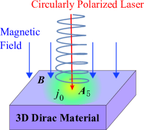
Figure 1: Experimental setup with the magnetic field and the circularly polarized laser onto a 3D Dirac semimetal.

II Floquet effective Hamiltonian and axial-vector field

We explain how to realize the axial-vector field in a 3D gapless Dirac system by applying a circularly polarized laser. We note that concrete calculations below are known ones, but a clear recognition of the axial-vector field has not been established. When continuous laser fields are imposed externally, the Hamiltonian $H(t)$ becomes periodically time-dependent, i.e., $H(t+T)=H(t)$ where $T=2\pi/\Omega$ is the periodicity. Quantum states in time periodic driving are described by the Floquet theory Sambe:1973 ; Shirley:1965 , that is, a temporal version of the Bloch theorem. The essence of the Floquet theory is a mapping between the time-dependent Schrödinger equation and a static eigenvalue problem. The eigenvalue is called the Floquet pseudo-energy and plays a role similar to the energy in a static system. Applications of the Floquet theory to periodically driven systems with topology changing has been a recent hot topic Oka09 ; Kitagawa11 ; Lindner11 ; Wang:2014 and experiments have also been done Karch10 ; Karch11 ; Wang13 ; Jotzu14 .

To make this paper as self-contained as possible, in this section, we derive the effective Hamiltonian in an explicit way, though the final result is not very new but already known. Let us consider a Hamiltonian, $H_{\rm tot}=H_{0}+H_{\rm int}$, with

$$H_{0}=\gamma^{0}\boldsymbol{\gamma}\cdot\boldsymbol{p}+\gamma^{0}m\;,\qquad H_{\rm int}=-e\gamma^{0}\boldsymbol{\gamma}\cdot\boldsymbol{A}\;,$$ (3)

that describes the one-particle Dirac system coupled to an external gauge field and $\gamma^{\mu}$ are the Dirac matrices satisfying $\{\gamma^{\mu},\gamma^{\nu}\}=2\eta^{\mu\nu}$. In an electric field with circular polarization in the $x$-$y$ plane, we can write the time-dependent vector potentials down as

$$A_{x}=\frac{E_{0}}{\Omega}\cos(\Omega t)\;,\quad A_{y}=\frac{E_{0}}{\Omega}\sin(\Omega t)\;\quad A_{z}=0\;,$$ (4)

where $\Omega$ is the frequency. We can conveniently decompose the interaction part of the Hamiltonian into two pieces as $H_{\rm int}=e^{i\Omega t}H_{-}+e^{-i\Omega t}H_{+}$ where $H_{\pm}=-(eE/\Omega)\gamma^{0}\gamma^{\pm}$ with $\gamma^{\pm}=\frac{1}{2}(\gamma^{x}\pm i\gamma^{y})$. Now we assume that the the period $T=2\pi/\Omega$ of the circular polarization is small enough as compared to the typical observation timescale. We can then expand the theory in terms of $\omega/\Omega$ (with $\omega$ being a frequency corresponding to some excitation energy). Taking the average over $T$ we can readily find the following effective Hamiltonian Haeberlen:1968zz ; Blanes:2009 ; Kitagawa10 ; Kitagawa11 :

$$H_{\text{eff}}=\frac{i}{T}\ln\Bigl{[}\mathcal{T}e^{-i\int_{0}^{T}dt\,H(t)}\Bigr{]}\simeq H_{0}+\frac{1}{\Omega}[H_{-},H_{+}]\;,$$ (5)

to the first order in the expansion. We can also find the same form from the Floquet Hamiltonian using the Van Vleck perturbation theory Vleck:1929 . Interestingly we can express the induced term as

$$H_{\text{ind}}\equiv\frac{1}{\Omega}[H_{-},H_{+}]=-\frac{(eE_{0})^{2}}{\Omega^{3}}i\gamma^{x}\gamma^{y}=-\beta\gamma^{0}\gamma^{z}\gamma_{5}\;,$$ (6)

where we defined $\beta\equiv(eE)^{2}/\Omega^{3}$. This means that the circular polarized electric field would induce an axial-vector background field $\boldsymbol{A}_{5}=\beta\hat{\boldsymbol{z}}$ perpendicular to the polarization plane. Essentially the same expression was obtained in the context of “Floquet Weyl semimetal” and the corresponding Floquet bands were figured out Wang:2014 . The physics is basically the same as this preceding work Wang:2014 , but we use a different language here and, for completeness, we shall see the energy dispersion relations in the rest of this section.

The effect of finite $\beta$ is easily understandable from the energy dispersion relations. We can immediately diagonalize $H_{\text{eff}}$ and the four pseudo-energies read:

$$\varepsilon_{\pm}(p)=\sqrt{p_{x}^{2}+p_{y}^{2}+(\sqrt{p_{z}^{2}+m^{2}}\pm\beta)^{2}}$$ (7)

and $-\varepsilon_{\pm}(p)$. We display low-lying $\pm\varepsilon_{-}(p)$ in Fig. 2. which shows that the Dirac point splits into two Weyl points with a displacement given by

$$\Delta p=\sqrt{\beta^{2}-m^{2}}\;.$$ (8)

In fact, $\beta$ is nothing but a momentum shift along the $z$-axis that is positive for the right chirality state (i.e., $\gamma_{5}\psi_{\rm R}=+\psi_{\rm R}$) and negative for the left chirality state (i.e., $\gamma_{5}\psi_{\rm L}=-\psi_{\rm L}$). We point out that time-resolved ARPES should be able to see this splitting of Weyl points in a similar manner as the gap opening Oka09 of the 2D Dirac point already observed experimentally Wang13 . Interestingly, as long as $\beta>m$, the pseudo-energy always has two Weyl points (if they are inside of the Brillouin zone) even for $m>0$. Therefore, we do not have to require strict massless-ness to realize gapless dispersions, which should be a quite useful feature for practical applications including the Schwinger or Landau-Zener effect. In what follows below, we limit ourselves to the $m=0$ case just for technical simplicity.

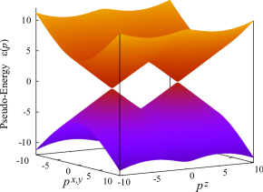
Figure 2: Pseudo-energies $\pm\varepsilon_{-}(p)$ as a function of $p^{x,y}=\sqrt{p_{x}^{2}+p_{y}^{2}}$ and $p^{z}$ for $\beta>m$ [in the figure $(m,\beta)=(1,5)$ was chosen].

The generalization from the one-particle Hamiltonian to the many-body field theory is straightforward. It is then more convenient to work with the Lagrangian density corresponding to $H_{\text{eff}}$, that we can express as

$$\mathcal{L}_{\text{eff}}=\bar{\psi}(\hbox to5.03125pt{\hbox to0.0pt{\hbox to5.03125pt{\hss/\hss}\hss}\hbox{$p$}}-m)\psi+\beta\bar{\psi}\gamma^{z}\gamma_{5}\psi+\mu_{\rm A}\bar{\psi}\gamma^{0}\gamma_{5}\psi\;.$$ (9)

Here we include $\mu_{\rm A}$ for completeness, which is a necessary ingredient for the CME.  It is clear from this Hamiltonian that we should identify $\beta$ as a parameter representing what is called the chiral shift Gorbar:2009bm ; Gorbar:2010kc . We should emphasize a crucial difference from the idea of the chiral shift that is not directly controllable but secondarily generated by finite-density effects. In our present problem, however, $\beta$ is an external parameter that we can control with the amplitude and/or the frequency of the circular polarized electric field. What we will see is that, conversely to discussions on the chiral shift Gorbar:2009bm ; Gorbar:2010kc , a finite density is generated by this externally given $\beta\neq 0$.

III Response to the magnetic field

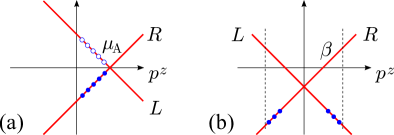
Figure 3: Energy dispersion relations of the LLL (i.e., $p^{x}=p^{y}=0$) with (a) chiral chemical potential $\mu_{\rm A}$ relevant for the CME and (b) chiral shift $\beta$ relevant for the CPE.  Filled (blank) dots represent states that are newly occupied (unoccupied).

It is the most essential point that we can regard $\beta$ as the $z$ component of an axial-vector field; $\beta\sim A_{5}^{z}$. Then, if we further impose an external magnetic field $B^{z}=F^{12}$ on this system, we should expect the following anomaly relation; $j^{0}\;\propto\;\beta B$, immediately from the CPE or Eq. (2). We will confirm this expectation with explicit calculations, but before going into details, let us consider an intuitive interpretation to understand Eq. (2).

For the purpose of comprehensible illustration it would be useful to sketch the dispersion relations in the same way as in a CME literature Fukushima:2008xe . Figure 3 (a) shows the dispersion relations of the lowest Landau levels (LLLs) relevant for the CME with $\beta=0$ and $\mu_{\rm A}\neq 0$. In this case with $\mu_{\rm A}>0$ the energies of the right-handed ($R$) particles are decreased, while those of the left-handed ($L$) particles are increased. Note that only one spin state is chosen out for the LLL depending on the sign of $eB$. Therefore, a positive $\mu_{\rm A}$ favors more $R$ than $L$. This explains how a finite chiral density is accumulated, while a net density remains vanishing. Also we see that the CME current flows from the LLL with $\mu_{\rm A}$ and gives an intuitive picture for the anomaly relation (1). In contrast, as seen in Fig. 3 (b) for $\beta>0$, the energy dispersion of $R$ (and $L$) is shifted positively (and negatively, respectively) along the $p^{z}$ axis. Thus, assuming that particles can flow in through the $p^{z}$-integration edges [as indicated by the dashed lines in Fig. 3 (b)], both $L$ and $R$ LLL states increase their occupation. This is the mechanism of how a finite density develops from a combination of $\beta$ and $B$ (that causes the dimensional reduction) through the anomaly relation (2). The argument at the same time tells us that a $R$ excess in $p_{z}<0$ and an $L$ excess in $p_{z}>0$ contribute to a negative flow of the net chirality, which is an analogue of the CME current. Summarizing the above discussions we should expect non-zero $\langle j^{0}\rangle$ and $\langle j_{\rm A}^{z}\rangle$.

Now we shall make sure of our qualitative argument by performing explicit calculations and identify the coefficient of Eq. (2) following the calculations done previously Gorbar:2009bm ; Gorbar:2010kc . We set $\mu_{\rm A}=0$ in the following and concentrate on the CPE only. The fermion propagator with $\beta$ in the presence of $eB>0$ is

$$G(x\sim 0)\simeq G_{0}^{-}(x)P_{-}+\sum_{n=1}^{\infty}[G_{n}^{+}(x)P_{+}+G_{n}^{-}(x)P_{-}]$$ (10)

near the coincidence limit, where $P_{\pm}\equiv\frac{1}{2}(1\pm i\gamma^{x}\gamma^{y})$ is the spin projection operator and the first term, $G_{0}^{-}P_{-}$, is the LLL contribution. The (Feynman) propagator for each Landau mode is

$$G_{n}^{\pm}(x\sim 0) =\frac{ieB\gamma^{0}}{2\pi}\int\frac{d\omega\,dp}{(2\pi)^{2}}\Bigl{[}K_{n}(\omega,\pm(p+\beta))P_{5}^{-}$$

$$\qquad\qquad+K_{n}(\omega,\mp(p-\beta))P_{5}^{+}\Bigr{]}\;.$$ (11)

Here, $P_{5}^{\pm}\equiv\frac{1}{2}(1\pm\gamma_{5})$ is the chirality projection operator and we defined

$$K_{n}(\omega,p)=\frac{\omega+p}{\omega^{2}-2eBn-p^{2}+i\epsilon}\;.$$ (12)

Using this form of the propagator we can express the current expectation value as

$$\langle j^{0}\rangle=-e\,\lim_{t\to 0^{+}}\mathrm{tr}[\gamma^{0}G(t)]\;.$$ (13)

We can simplify the calculation by noting that $\mathrm{tr}(P_{5}^{\pm}P_{\pm})=\frac{1}{4}\mathrm{tr}[(1\pm\gamma_{5})(1\pm i\gamma^{x}\gamma^{y})]=1$ where two $\pm$ are independent. Because $\omega$ in the numerator should be vanishing after the $\omega$ integration, it is straightforward to check that $\mathrm{tr}(\gamma^{0}G_{n}^{+}P_{+})+\mathrm{tr}(\gamma^{0}G_{n}^{-}P_{-})=0$. Therefore only the LLL contribution survives, which yields:

$$\langle j^{0}\rangle=-\frac{e^{2}B}{2(2\pi)}\int\frac{dp}{2\pi}\biggl{(}-\frac{p+\beta}{|p+\beta|}+\frac{p-\beta}{|p-\beta|}\biggr{)}$$ (14)

after the $\omega$ integration. The above is a finite integral only from $-\beta\leq p_{z}\leq\beta$. Actually, this simple expression is precisely a concrete realization of our qualitative argument based on Fig. 3 (b). Finally, after the $p$ integration, we recover the same result as previously obtained one Gorbar:2009bm :

$$\langle j^{0}\rangle=\frac{e^{2}\beta B}{2\pi^{2}}\;,$$ (15)

which is quite reminiscent of the formula for the CME current, namely, $\langle j^{z}\rangle=e^{2}\mu_{\rm A}B/(2\pi^{2})$. This compact formula itself is a known one, but the fact that the above $\langle j^{0}\rangle$ can be easily realized with a circularly polarized laser is our main claim in this work.

Remembering our qualitative argument, we can in turn expect an axial current $\langle j_{\rm A}^{z}\rangle$ which is similar to what is called the chiral separation effect; $\langle j_{\rm A}^{z}\rangle\propto\mu B$ Metlitski:2005pr . To see this, let us perform an explicit calculation using $\langle j_{\rm A}^{z}\rangle=-e\,\mathrm{tr}[\gamma^{z}\gamma_{5}G(0^{+})]$. In this case we use $\mathrm{tr}(\gamma^{z}\gamma_{5}\gamma^{0}P_{5}^{\pm}P_{\pm})=\frac{1}{4}\mathrm{tr}[\gamma^{z}\gamma_{5}\gamma^{0}(1\pm\gamma_{5})(1\pm i\gamma^{x}\gamma^{y})]=\pm\frac{i}{4}\mathrm{tr}(\gamma^{z}\gamma_{5}\gamma^{0}\gamma^{x}\gamma^{y})=\pm 1$, where the last $\pm$ refers to $\pm$ of $P_{\pm}$. Then, the LLL contribution is completely identical to that for $\langle j^{0}\rangle$ except for the overall sign, that means, $\langle j_{\rm A}^{z}\rangle_{\text{(LLL)}}=-\langle j^{0}\rangle$. We can immediately explain this proportionality for the LLL from the property of the two-dimensional Dirac matrices; $\gamma^{z}\gamma_{5}^{(2)}=\gamma^{0}$ where $\gamma_{5}^{(2)}$ is the two-dimensional counterpart defined by $\gamma^{0}\gamma^{z}$. In this case, however, some complication appears from non-zero Landau levels as is the case for the chiral shift Gorbar:2009bm ; Gorbar:2010kc . We can write those contributions down explicitly as

$$\begin{split}&\langle j_{\rm A}^{z}\rangle_{(n>0)}=\frac{e^{2}B}{2\pi}\int\frac{dp}{2\pi}\sum_{n}\\ &\times\biggl{(}-\frac{p+\beta}{\sqrt{2eBn+(p\!+\!\beta)^{2}}}+\frac{p-\beta}{\sqrt{2eBn+(p\!-\!\beta)^{2}}}\biggr{)}\;.\end{split}$$ (16)

This is a subtle expression whose precise value depends on how to organize the infinity in the Landau sum and the momentum integration. For example, if we take the Landau sum up to $N$ and the momentum integration within $|p|<\Lambda$ in such a way that $2eBN\ll\Lambda^{2}$, then the $p$ integration is easy to perform and we find $\langle j_{\rm A}^{z}\rangle_{(n>0)}=-2N\langle j^{0}\rangle$. For more general situation $N$ should be replaced with $(\Lambda/eB)(\sqrt{2eBN+\Lambda^{2}}-\Lambda)$, which approaches $\sqrt{2N\Lambda^{2}/eB}$ in the opposite limit of $\Lambda^{2}\ll 2eBN$. In reality these cutoffs should be fixed by the microscopic properties of the material, especially the Debye mass and the Brillouin zone structures. The conclusion is that the system comes to have a finite axial-current as given by

$$\langle j_{\rm A}^{z}\rangle=-\alpha\,\frac{e^{2}\beta B}{2\pi^{2}}\;,$$ (17)

the coefficient $\alpha$ of which is not anomaly protected unlike Eq. (15) and it is a material-dependent problem to fix $\alpha$.

IV Static charge distribution

So far, we assumed an infinitely large system. Imposing surface boundary conditions with a finite extent, we should take account of the polarization and screening effects to find a balanced distribution of the charge and the chirality density. Let us consider a finite-size material whose thickness in the $z$ direction is $d$; we take the $z$ coordinate so that the material is placed in a range $-d/2\leq z\leq+d/2$. Then, because of the surface effects, we should introduce $z$ dependent $\mu(z)$ and $\mu_{\rm A}(z)$, the determination of which is the goal of this section.

In the presence of $\mu_{\rm A}(z)$, the CME current should follow from Eq. (1). In equilibrium, however, there should be no current and the CME current should be canceled by the polarization effect, i.e.

$$j^{z}_{\rm total}=\frac{e^{2}B}{2\pi^{2}}\mu_{\rm A}(z)+\sigma\int dz\,j^{0}(z)\;,$$ (18)

where the second term in the right-hand side appears from Ohm’s law with the electric conductivity $\sigma>0$. In fact, $\int dz\,j^{0}(z)$ is nothing but an electric field associated with the polarization or the charge distribution $j^{0}(z)$. Qualitatively, this last term represents a flow to flatten the charge distribution. For the balance equation for $j_{\rm A}^{z}$ we postulate the same structure as Eq. (18) with the replacement of $j^{\mu}\leftrightarrow j_{\rm A}^{\mu}$ and $\mu\leftrightarrow\mu_{\rm A}$ (i.e., the chiral separation effect Metlitski:2005pr ):

$$j_{\rm A\,,total}^{z}=\frac{e^{2}B}{2\pi^{2}}\mu(z)-\frac{e^{2}B}{2\pi^{2}}\alpha\beta-\lambda\partial_{z}j_{\rm A}^{0}(z)\;,$$ (19)

where we added the last term to consider diffusion processes of chirality introducing a diffusion constant $\lambda>0$. Intuitively, this last term represents movement of chirality to decrease the chirality gradient. The densities, $j^{0}$ and $j_{\rm A}^{0}$, are given as

$$j^{0}=\frac{e^{2}B}{2\pi^{2}}\beta+\frac{e}{3\pi^{2}}\mu(z)^{3}\;,\qquad j_{\rm A}^{0}=\frac{e}{3\pi^{2}}\mu_{\rm A}(z)^{3}\;,$$ (20)

where a CPE contribution to $j^{0}$ is added to the standard density-chemical potential relation. We plug these expressions to the conservation laws; $\partial_{\mu}j^{\mu}=0$ and $\partial_{\mu}j_{\rm A}^{\mu}=0$ (note that there is no $\boldsymbol{E}\cdot\boldsymbol{B}$ with our electromagnetic configuration). Since we are interested in the static profile only, we can drop the time-derivatives to reach finally:

$$\frac{e^{2}B}{2\pi^{2}}\partial_{z}\mu_{\rm A}(z)+\sigma\frac{e^{2}B}{2\pi^{2}}\beta+\frac{e\sigma}{3\pi^{2}}\mu(z)^{3}=0\;,$$ (21)

$$\frac{e^{2}B}{2\pi^{2}}\partial_{z}\mu(z)-\frac{e\lambda}{3\pi^{2}}\partial_{z}^{2}\mu_{\rm A}(z)^{3}=0\;.$$ (22)

We should solve these differential equations under the charge constraint; $\int_{-d/2}^{d/2}dz\,j^{0}(z)=(e^{2}B/2\pi^{2})\beta d$, which leads to $\mu_{\rm A}(d/2)-\mu_{\rm A}(-d/2)=-\beta\sigma d$. If the thickness $d$ of the material is sufficiently small, we can find an approximate solution by expanding the solutions in terms of $z$, that is,

$$\mu(z)\simeq-\frac{2\beta^{3}\sigma^{3}\lambda}{eB}z^{2}\;,\qquad\mu_{\rm A}(z)\simeq-\beta\sigma z\;.$$ (23)

Here, we further used a condition to impose zero net chirality. It should noted that these are leading-order results and, to satisfy Eq. (21) strictly for example, we should consider a term $\propto z^{7}$ in $\mu_{\rm A}(z)$ which we neglected. The charge density is thus more screened near the surface at larger $|z|$ unlike an ordinary conductor, while there are more $R$ (and $L$) near the bottom at negatively large $z$ (and near the top at positively large $z$, respectively). This is very interesting result; the system behaves as a capacitor of chirality or the chiral battery in which a non-zero slope in the chirality distribution is sustained by the CPE as well as a finite net density. Such a realization of the chiral battery should be useful for more quantitative investigations of the CME and related phenomena, e.g., the chiral plasma instability Akamatsu:2013pjd for instance. We note that the idea of the chiral battery can be traced back to the original work Fukushima:2008xe and extensively discussed as chiral electronics Kharzeev:2013 .

V Discussions and summary

The anomalously induced charge density $\langle j^{0}\rangle$ given by Eq. (2) or (15) is an experimentally detectable quantity. One possible way to observe this is using transient grating techniques Gedik:2003 . The grating of the circular polarized field would lead to inhomogeneous charge distribution, and the dynamics afterward can be measured.

It is also an interesting possibility to make use of Eq. (17) instead of Eq. (15) since $\alpha$ could take a large number (involving some cutoffs at least in a naive estimate). In the two-component spinor representation, $j_{\rm A}^{z}=\phi^{\ast}_{\rm R}\sigma^{z}\phi_{\rm R}+\phi^{\ast}_{\rm L}\sigma^{z}\phi_{\rm L}$ is nothing but the spin expectation value. Hence, for systems with gapless Dirac particles, Eq. (17) indicates not only the dynamical flow of chirality but also the spin polarization. Spin polarization can be probed by pump-probe magneto-optical Kerr effect. In addition, when topological current or density exists in general, there can be some photo-emission processes via anomaly as discussed in Refs. Basar:2012bp ; Fukushima:2012fg . It deserves further investigations to quantify emitted photon spectra associated with the CME and the CPE.  We will leave them for interesting future problems.

In summary, we formulated the CPE that generates a finite density from the combination of the circular polarized electric field and the magnetic field. The interesting point in this setup is that the externally imposed electric and magnetic fields are always pointing orthogonal to each other and there is no inner product of $\boldsymbol{E}\cdot\boldsymbol{B}$ which is usually the source of topological charge and parity breaking. Instead, the circular polarization breaks the parity symmetry, and so it alone can take care of the role of $\boldsymbol{E}\cdot\boldsymbol{B}$. Besides, thanks to rotating electric field, we do not need to subtract a huge background due to ordinary electric current that obeys Ohm’s law.

We gave intuitive arguments about the generation of the density and the axial current and confirmed our expectations by explicit calculations recovering previously known expressions. We saw that the density $\langle j^{0}\rangle$ is expressed in a compact form similar to the CME and its coefficient is anomaly protected. In contrast to this, $\langle j_{\rm A}^{z}\rangle$ has complicated contributions that need some ultraviolet regularization or physical cutoff. We would here emphasize the following point: Each building block for our conclusion was known; the appearance of a $\gamma^{x}\gamma^{y}$ term from the Floquet Weyl semimetal and the topologically induced density from the chiral shift were all “re-derived” in this work, but our novelty is found in a combination of them. The most important is that our controlling parameter $\beta$ is given externally unlike the axion term associated with intrinsic properties of the material.

Although it is difficult to determine the coefficient of $\langle j_{\rm A}^{z}\rangle$, it is still proportional to $\beta$ or a combination of $(eE)^{2}/\Omega^{3}$ (as long as $\Omega$ is large enough to justify the leading-order expansion as we did in this work). This characteristic dependence of $\Omega^{-3}$ should give a consistency check for anomalously induced $\langle j^{0}\rangle$ and $\langle j_{\rm A}^{z}\rangle$.

Fortunately, such ambiguity in $\langle j_{\rm A}^{z}\rangle$ does not enter the determination of the static charge and chirality distribution in the material. Our study implies that the induced $\langle j^{0}\rangle$ gets slightly smaller near the material surfaces. The most interesting is that the chirality has a non-trivial distribution also and the chirality separation is sustained by the CPE, which realizes a system of the chiral battery. The experimental confirmation of the CPE itself is quite challenging, and furthermore, the CPE opens a new possibility for more direct CME studies using this chiral battery.

- (1) S. Adler, Phys. Rev. 177, 2426 (1969).
- (2) J. S. Bell, and R. Jackiw, Nuovo Cimento 60A, 4 (1969).
- (3) D. E. Kharzeev, L. D. McLerran and H. J. Warringa, Nucl. Phys. A 803, 227 (2008).
- (4) K. Fukushima, D. E. Kharzeev and H. J. Warringa, Phys. Rev. D 78, 074033 (2008).
- (5) B. I. Abelev et al. [STAR Collaboration], Phys. Rev. Lett. 103, 251601 (2009); B. Abelev et al. [ALICE Collaboration], Phys. Rev. Lett. 110, 012301 (2013).
- (6) Z. Wang et al., Phys. Rev. B 85, 195320 (2012).
- (7) Z. Wang, H. Weng, Q. Wu, X. Dai, and Z. Fang, Phys. Rev. B 88, 125427 (2013).
- (8) M. Neupane et al., Nat. Phys. 5, 4086 (2014)
- (9) Z.K. Liu et al., Nat. Mat. 13, 677–681 (2014).
- (10) J. Cao et al., Nat. Com. 6, 7779 (2015)
- (11) L. X. Yang et al., Nat. Phys. 10, 3425 (2015)
- (12) B. Lv et al., Nat. Phys. 10, 3426 (2015)
- (13) S. Y. Xu et al., Nat. Phys. 10, 3437 (2015)
- (14) Q. Li et al., arXiv:1412.6543 [cond-mat.str-el].
- (15) M.M. Vazifeh and M. Franz, Phys. Rev. Lett. 111, 027201 (2013).
- (16) Z. Wang and S.-C. Zhang, Phys. Rev. B 87, 161107 (2013).
- (17) F. Wilczek, Phys. Rev. Lett. 58, 1799 (1987).
- (18) A.A. Zyuzin and A.A. Burkov, Phys. Rev. B 86, 115133 (2012).
- (19) A. Narayan, Phys. Rev. B 91, 205445 (2015).
- (20) C.-K. Chan, P.A. Lee, K.S. Burch, J.H. Han, and Y. Ran, arXiv:1509.05400 [cond-mat.mes-hall].
- (21) H. B. Nielsen, M. Ninomiya, Phys. Lett. 130B, 389 (1983)
- (22) V. Schon and M. Thies, In *Shifman, M. (ed.): At the frontier of particle physics, vol. 3* 1945-2032 [hep-th/0008175].
- (23) H. Sambe, Phys. Rev. A 7, 2203 (1973).
- (24) J.H. Shirley, Phys. Rev. B 138, 979 (1965).
- (25) T. Oka and H. Aoki, Phys. Rev. B 79, 081406 (2009).
- (26) T. Kitagawa, T. Oka, A. Brataas, L. Fu, and E. Demler, Phys. Rev. B 84, 235108 (2011).
- (27) N. H. Lindner, G. Refael, and V. Galitski, Nat. Phys. 7, 490 (2011).
- (28) R. Wang, B. Wang, R. Shen, L. Sheng and D. Y. Xing, EPL 105, 17004 (2014).
- (29) J. Karch, et al. , Phys. Rev. Lett. 105, 227402 (2010).
- (30) J. Karch, et al. , Phys. Rev. Lett. 107, 276601 (2011).
- (31) Y. H. Wang, H. Steinberg, P. Jarillo-Herrero, and N. Gedik, Science, 342, 453 (2013).
- (32) G. Jotzu, M. Messer, Rémi Desbuquois, M. Lebrat, T. Uehlinger, D. Greif, and T. Esslinger, Nature 515, 237 (2014).
- (33) T. Kitagawa, M. S. Rudner, E. Berg, and E. Demler, Phys. Rev. A 82, 0033429 (2010).
- (34) U. Haeberlen and J. S. Waugh, Phys. Rev. 175, 453 (1968).
- (35) S. Blanes, F. Casas, J.A. Oteo and J. Ros, Phys. Rept. 470, 151–238 (2009).
- (36) J. H. Van Vleck, Phys. Rev. 33, 467 (1929).
- (37) E. V. Gorbar, V. A. Miransky and I. A. Shovkovy, Phys. Rev. C 80, 032801 (2009); Phys. Rev. D 83, 085003 (2011).
- (38) E. V. Gorbar, V. A. Miransky and I. A. Shovkovy, Phys. Lett. B 695, 354 (2011).
- (39) M. A. Metlitski and A. R. Zhitnitsky, Phys. Rev. D 72, 045011 (2005).
- (40) Y. Akamatsu and N. Yamamoto, Phys. Rev. Lett. 111, 052002 (2013).
- (41) D.E. Kharzeev and H.-U. Yee, Phys. Rev. B 88, 115119 (2013).
- (42) N. Gedik, J. Orenstein, R. Liang, D.A. Bonn, W.N. Hardy, Science 300, 1410 (2003).
- (43) G. Basar, D. Kharzeev and V. Skokov, Phys. Rev. Lett. 109, 202303 (2012).
- (44) K. Fukushima and K. Mameda, Phys. Rev. D 86, 071501 (2012).