Quantifying the Carbon Abundances in the Secondary Stars of SS Cygni, RU Pegasi, and GK Persei

Abstract

We use a modified version of MOOG to generate large grids of synthetic spectra in an attempt to derive quantitative abundances for three CVs (GK Per, RU Peg, and SS Cyg) by comparing the models to moderate resolution (R $\sim$ 25,000) $K$-band spectra obtained with NIRSPEC on Keck. For each of the three systems we find solar, or slightly sub-solar values for [Fe/H], but significant deficits of carbon: for SS Cyg we find [C/Fe] = $-$0.50, for RU Peg [C/Fe] = $-$0.75, and for GK Per [C/Fe] = $-$1.00. We show that it is possible to use lower resolution (R $\sim$ 2,000) spectra to quantify carbon deficits. We examine realistic veiling scenarios and find that emission from H I or CO cannot reproduce the observations.

Key words: infrared: stars — stars: cataclysmic variables — stars: individual (SS Cyg, RU Peg, GK Per) — stars: abundances

1 Introduction

Cataclysmic Variables (CVs) are a diverse group of short-period binaries in which a late-type, Roche-lobe filling secondary star transfers matter through an accretion disk onto a white dwarf primary. The standard paradigm for the formation of CVs postulates that they start out as wide binaries (on the order of 1 AU), of moderate orbital period ($<<$ 1 yr). As the more massive component, the white dwarf progenitor, evolves off of the main sequence, the secondary star suddenly finds itself orbiting within the red giant photosphere. During this “common envelope” (CE) phase, much of the angular momentum of the binary is believed to be shed due to interactions of the secondary star with the atmosphere of the red giant. During this process, the binary period gets shortened, and the red giant envelope gets ejected. Depending on the input parameters used in standard CE models, between 50 and 90% of all of these close binary stars merge (c.f., Politano & Weiler 2007). After emerging from the CE phase, an epoch of angular momentum loss via magnetic braking (Verbunt & Zwaan 1981), lasting $\approx$ 10^-7 yr (Warner 1995), is then required that leads to the formation of a semi-detached binary, and the mass transfer phase that signals the birth of a CV.

In this scenario, the vast majority of CV secondary stars should not show any signs of evolution, as there just has not been sufficient time for the low mass secondary stars (M₂ $\leq$ 1 M_☉) in these systems to have begun to evolve off of the main sequence. Thus, the composition of the secondary stars should be relatively normal unless they have accreted matter with an unusual composition during the CE phase, or perhaps during classical novae eruptions. In an infrared spectroscopic survey of CVs, Harrison et al. (2004, 2005) found that the CO features of the secondary stars in a number of CVs were much weaker than expected for their spectral types. For U Gem, the CO features were extremely weak, yet the water vapor feature was normal for a spectral type of M4V. This suggested a deficit of carbon. Hamilton et al. (2011) have tabulated the list of CVs with weaker than expected CO features, and show that, when such data exists, analysis of UV spectra also find evidence for carbon deficiencies. One issue with the infrared spectroscopy surveys was that they were qualitative, and were derived from lower resolution (R $\sim$ 2000) spectroscopy. The line features in those spectra might be compromised due to veiling by a continuum source that arises from the accretion disk.

We have obtained moderate, and lower resolution, $K$-band spectroscopy of three of the brightest CVs: SS Cyg, RU Peg, and GK Per. Previous near-infrared spectroscopy with SPEX (Harrison et al. 2004, 2007) revealed that the secondary stars in these three systems had weaker than expected CO features. In the following, we use a modified version of the MOOG spectral synthesis program to model moderate resolution $K$-band spectra to examine the atomic and molecular abundances in their secondary stars. As shown in Hamilton et al. (2011), higher resolution spectra dramatically reduce the effects of accretion disk veiling, allowing us to see secondary stars even in CV systems where the accretion luminosity totally dominates that of the secondary star. In the systems discussed here, however, the secondary star dominates the accretion disk flux in the $K$-band, and any veiling has to be quite small. We then compare the best fit model spectra derived from the higher resolution data to lower resolution data.

In the next section we discuss the data to be modeled, in section 3 we discuss the spectral synthesis procedure, in section 4 we present the modeling of the data, discuss the results in section 5 and draw our conclusions in section 6.

2 Observations

SS Cyg, RU Peg, and GK Per were observed using NIRSPEC in high resolution mode on Keck II on 2004 August 28. The 0.432 x 12″ slit was used providing a resolving power of R $\sim$ 25000, or a velocity resolution of $\Delta v$ $\sim$ 12 km s^-1. We employed the two-nod script, and we used five minute exposure times for the three program CVs. To completely cover the $K$-band using NIRSPEC requires two grating settings. Due to time limitations, however, we only obtained data at a single grating position chosen to insure coverage of the first overtone bandhead of ¹²CO_(2,0) at 2.294 $\mu$m. This grating setting also covers the ¹²CO_(5,3) bandhead at 2.383 $\mu$m. In addition to the three program CVs, we also observed two late-type stars, $\epsilon$ Eri (K2V) and $\gamma$ Psc (G9III), to provide templates for our synthetic spectral program given that the properties of those two objects are well known.

To correct for telluric absorption, we observed bright A0V stars located close to the program objects so as to minimize their relative differences in airmass. These data were reduced using the IDL routine “$redspec$”, specially developed for NIRSPEC. In the $K$-band, the spectra of A0V stars are nearly featureless, except for the prominent H I Brackett $\gamma$ feature at 2.16 $\mu$m. The $redspec$ package does not attempt to correct for this feature, but can interpolate across such lines to reduce their impact upon division into the program star spectrum. Note that there is a weak telluric feature located very close to the Brackett $\gamma$ line, and thus the H I line profiles in spectra produced by the division of a “patched” A-star spectrum are slightly compromised.

Just prior to our observing run on Keck, we observed the three program CVs using SPEX at the IRTF on 2004 August 15. SPEX was used in cross-dispersed mode generating spectra spanning the range from 0.8 to 2.45 $\mu$m. In the $K$-band, the dispersion is 5.4 Å/pix. The raw data were reduced using SPEXTOOL (Cushing et al. 2004). A log of all of our observations is presented in Table 1, and includes the orbital phase at the mid-point of the observational sequence for each of the three CVs. The AAVSO light curve data base shows that SS Cyg was in quiescence at the time of both the SPEX and NIRSPEC observations, having reached visual maximum on 17 July. RU Peg was in outburst on 23 July, but was in quiescence for both observing runs. At the time of the infrared observations, GK Per had $V$ = 13.1, its normal minimum light value.

3 Spectral Synthesis and Stellar Atmosphere Modeling

To calculate a synthetic spectrum, three basic building blocks are required: A stellar atmosphere model, a list of atomic and molecular lines, and a tool to calculate the corresponding flux at the stellar surface as a function of wavelength. A full description of the modified version of MOOG and the grid generation and spectral matching Python code (called “kmoog”) used below is described in Hamilton (2013), here we highlight the most important aspects.

3.1 Model Atmospheres

There are several groups that provide precomputed atmosphere models, each with their own slightly different assumptions, simplifications, and basic input physics. Most of the models in general circulation, however, have the same underlying assumptions: The atmosphere is either modeled as a series of plane-parallel slabs (1D), or as a series of concentric shells (2D). The 1D and 2D atmosphere models are calculated assuming local thermodynamic equilibrium (LTE) conditions, in which one temperature can describe the particle velocity distribution as well as the population of atomic levels and ionization states around a given point in the stellar atmosphere. It is also assumed that the atmosphere is time invariant, with the effects of dynamical processes such as mixing and convection parameterized. Bonifacio et al. (2012) provide an overview of the more detailed assumptions and differences between the available atmosphere computation methods and programs. Recently, full 3D (radiation-hydrodynamic) stellar atmosphere models have been calculated across parameter grids (e.g., Ludwig et al. 2009, Hauschildt and Baron 2010, Magic et al. 2013a, 2013b). For this program, however, we have only used the 1D and 2D models.

The most commonly used atmosphere model codes are PHOENIX (Hauschildt et al. (1999), Allard et al. 2011), MARCS (Gustafsson et al. 1975, 2008), and ATLAS (Sbordone et al. 2004). PHOENIX is perhaps the most computationally sophisticated, sampling 42 million atomic and 550 million molecular lines when calculating opacity. MARCS model atmospheres are consistently updated through a web interface providing both 1D and 2D models. Ultimately for this project, we chose to use MARCS atmospheres. An important consideration for this choice was the existence of the interpolation code to create subgrid models, making it much simpler to construct a large grid of models quickly. Very recently, Mészáros et al. (2012) presented a new grid of atmospheres based off of ATLAS and MARCS codes with an updated H₂O line list as well as finer grid spacings in temperature, gravity, metallicity, and C and $\alpha$ abundances. Given their recent availability, however, all analyses and spectra computed here use solely the original MARCS grid.

3.2 Constructing an Input Line List

The next crucial step to constructing a synthetic spectrum is to assemble a list of atomic and molecular transitions for which you wish to calculate an opacity at the stellar surface. For our project we used the ATLAS line list with the addition of the CO line list by Goorvitch (1994). Each line list was converted into a common format before combining, and, in the case of the CO line list, only lines with $log_{10}(g_{\mathrm{f}})\geq-16$ and 2.28 $\leq\lambda\leq$ 2.405 $\mu$m were kept. The final list contains a total of 11,681 lines. For the purposes of this work, only computations involving diatomic molecules were considered. This eliminates lines of the important molecular species for the cooler M dwarfs commonly found in CVs, such as H₂O. As described below, synthetic spectra for the Sun and Arcturus were generated and compared to observations to provide the initial validation of this line list.

3.3 Spectral Synthesis Tool

There are a number of codes that can readily make use of MARCS and Kurucz atmospheres. MOOG (Sneden 1973) has one of the longest track records, and given its ubiquity, we chose it to compute the synthetic spectra for this work. When creating a spectrum, MOOG is internally limited to considering only 2500 lines in the line list. Given the size of our line list, we modified MOOG (see Hamilton 2013) to allow for lists of 250,000 lines. Two additional changes were made to the MOOG source code. First, a version was created to produce absolutely no output to the screen. This prevents unnecessary lag and slowdowns, as well as greatly enhances usability when running a large number of models simultaneously. Second, and most importantly, a new binary output file type of MOOG was created. Significant savings in storage size were realized by creating a true FITS output type, reducing the file size of a successfully created model by a factor of five or more. The FITS files created also have the benefit of being fully compliant and compatible with the standard CFITSIO libraries, unlike the FITS-like output already in the code. The FITS output created also has the benefit of storing both a full resolution spectrum as well as one convolved to lower resolutions, useful for quickly comparing against observations from different telescopes and instruments.

3.4 Validation of the Synthetic $K$-band Spectra

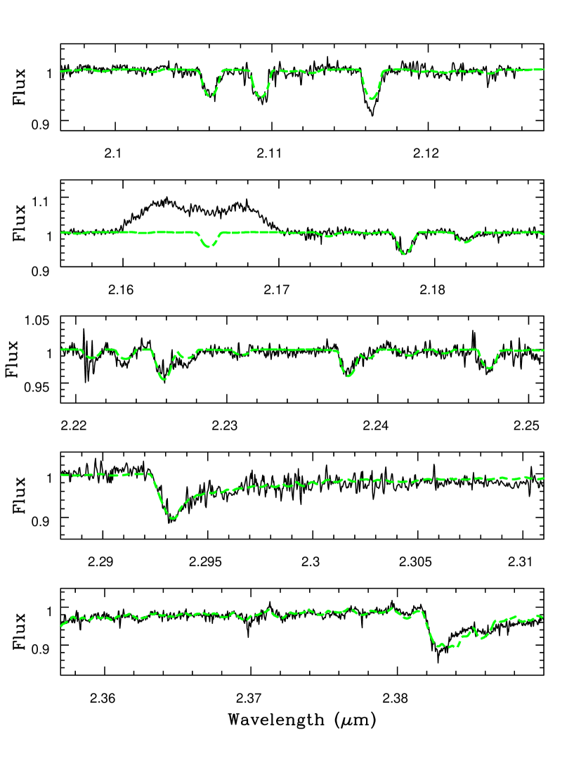
Figure 5: The NIRSPEC spectrum of SS Cyg (black) with the final best fitting synthetic spectrum overplotted (green). The template spectra have been rotationally broadened by 89 km s^-1. The broad emission feature at 2.165 $\mu$m is H I Br$\gamma$. The S/N ratio in these data ranged from 171 in the sixth order, to 67 in the second order.

To validate our line list, we constructed synthetic spectra for the Sun (using the solar MARCS model) and Arcturus (using the parameters listed in Table 2, but with log$g$ = 3.0) to compare them to high resolution $K$-band spectra published by Wallace et al. (1996), and Wallace & Hinkle (1996). We concentrated on the reproduction of only the strongest spectral features observed in these two objects. Note that the Arcturus comparison was only used to insure that we were not missing lines that become important at lower temperatures. We then altered the oscillator strengths of the most highly discrepant lines to insure that they would both fit the observations better, and not bias the automated fitting process. For example, there were a large number of Sc I transitions that had oscillator strengths that were much too large. Unfortunately, oscillator strengths for many of the transitions in the $K$-band do not appear in the NIST Atomic Spectra Database, and thus we used trial and error adjustment of the tabulated oscillator strength in the line list to better reproduce the observed spectral feature (for a primer on the identification of the strongest spectral features found in the $K$-band for K-type stars, see Fig. 5 in Harrison et al. 2004).

To test our ability to reproduce observations, we have constructed synthetic spectra to compare to the NIRSPEC observations of $\epsilon$ Eri and $\gamma$ Psc, and to a sample lower resolution spectra of K dwarfs contained in the IRTF Spectral Library (Cushing et al. 2009). We summarize the spectroscopically derived parameters for these objects in Table 2, averaging the data compiled in the PASTEL catalog (Soubiran et al. 2010) for each object, constrained to measures made after 1970. The final column of Table 2 denotes how many unique measurements went into the determination of each of the average properties for each star (note that HD45977 only has a single measurement of its characteristics by Sousa et al. 2011). As we will see, this sample more than spans the range in metallicity observed for our program CVs. Note that the solar abundance pattern derived by Grevesse et al. (2007) was used for all of the synthetic spectra, and only the abundance of carbon was altered for the investigation of the CVs.

In preparation for comparison to the models, the spectra were continuum normalized using a third order polynomial fit in IRAF. For the high resolution spectra, the process was quite trivial. For the full $K$-band spectra, however, we used an identical set of wavelength bins for identifying the continuum to be fit. The continua were then fitted over the range 2.08 to 2.29 $\mu$m, with bins that avoided all of the strongest spectral features.

3.4.1 $\epsilon$ Eri and $\gamma$ Psc

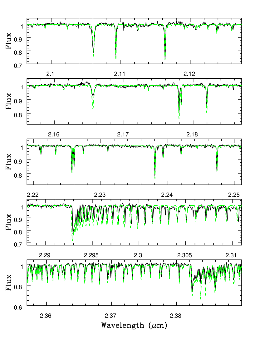
Figure 1: The NIRSPEC spectrum of $\epsilon$ Eri (black solid line). The synthetic model spectrum (green, dashed line) generated for this object is overplotted. For the purposes of this paper, the bottom panel will be defined as the second order, while the top panel will be labeled the sixth order. The synthetic spectrum has been rotationally broaded by 4 km s^-1 as measured by Martinez-Arnaiz et al. (2010). The S/N ratio ranged from 214 in the sixth order, to 95 in the second order.

The NIRSPEC spectrum of $\epsilon$ Eri is presented in Fig. 1, where data for five of the seven spectral orders are shown (the first order, spanning $\lambda$2.43 to 2.47 $\mu$m, was too far red to obtain appreciable signal in our CV spectra, while the seventh order spectrum is dominated by the strong telluric feature at 2.05 $\mu$m). As shown in Table 2, $\epsilon$ Eri has a temperature near 5100 K, and a near-solar metallicity of [Fe/H] = $-$0.1. In Fig. 1, we overplot a synthetic spectrum with T = 5100 K, and [Fe/H] = $-$0.125 (interpolated between the model atmospheres with [Fe/H] = $-$0.25, and [Fe/H] = 0.0). The model fit to the strongest lines is excellent. Note that we have inserted an H I Br$\gamma$ line into our line list. We do this to primarily show where this line is located. The profiles of this feature as found in the infrared spectra for each of the objects are unreliable due to the reduction technique. In addition, the profile of such a strong line cannot be easily reproduced using MOOG.

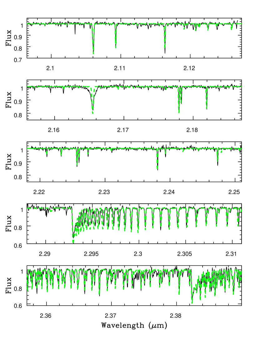
Figure 2: The NIRSPEC spectrum of $\gamma$ Psc (black) compared to a synthetic spectrum (green). The S/N ratio of these data ranged from 175 in the sixth order, to 75 in the second order.

$\gamma$ Psc allows us to test our ability to reproduce a much lower gravity object with a very low metallicity. We used a MARCS spherical, alpha-enhanced model atmosphere with log$g$ = 2.5, and [Fe/H] = $-$0.5 to generate a synthetic spectrum for $\gamma$ Psc. As noted in Alves-Brito et al. (2010), $\gamma$ Psc has a modest alpha-enhancement of $\sim$ $+$0.2, and thus many of the metal lines are stronger in $\gamma$ Psc than they would be in a model that has a solar abundance pattern. Since $kmoog$ does not yet have the capabilities to adjust the abundances of any other species besides carbon, we ran the MOOG binary used by $kmoog$ in a stand-alone mode, increasing the abundances of O, Al and Mg as detailed in Alves-Brito et al. We overplot this model on the observed data in Fig. 2. The resulting synthetic spectrum is a reasonable match to the data.

3.4.2 Comparison to the K Dwarfs in the IRTF Spectral Library

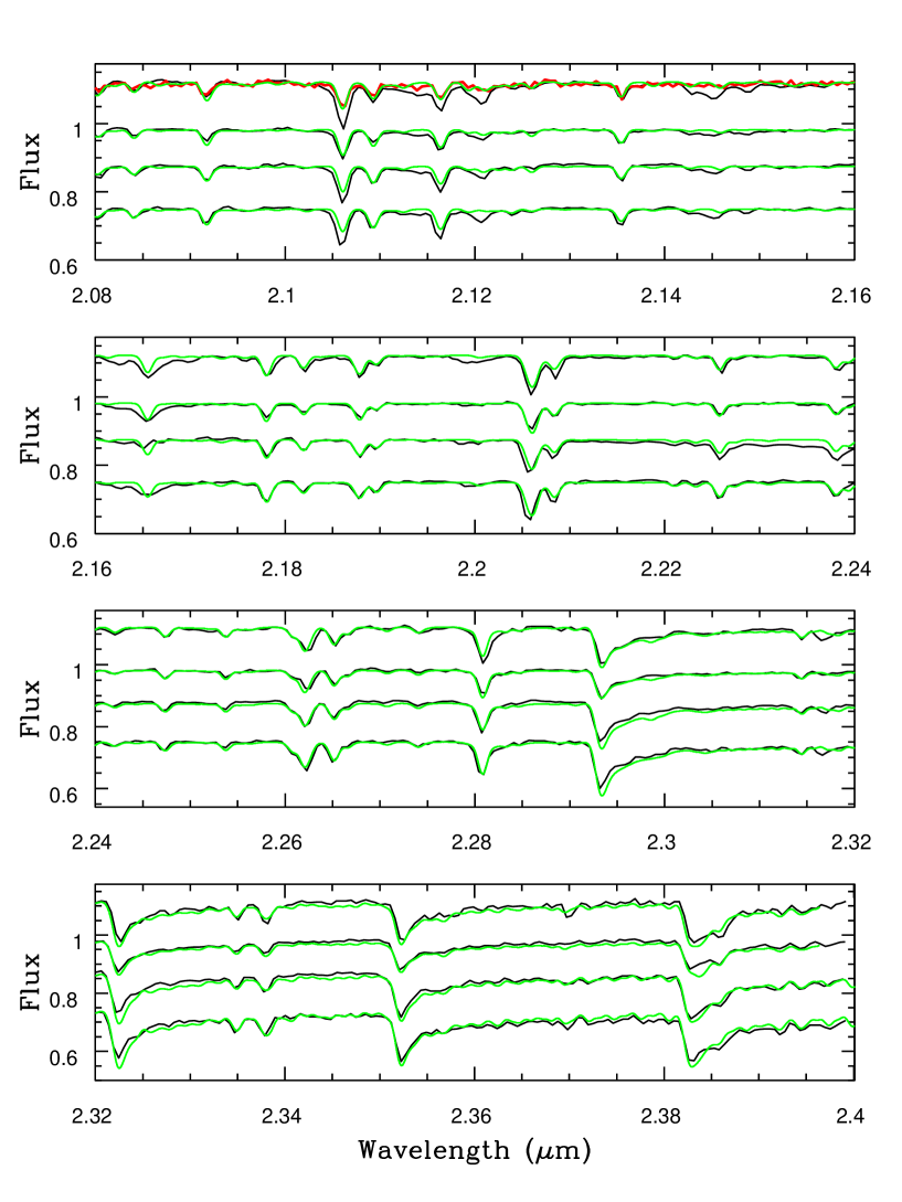
Figure 3: The SPEX spectra for K dwarfs spanning the range from K0V to K3V (black), along with synthetic spectra (green) generated for each of the objects using the parameters listed in Table 2. As described in the text, the template star spectra in the range 2.10 to 2.15 $\mu$m are not especially well matched by the models. The source of this discrepancy is hard to identify. In the top panel we also plot in red the spectrum of a G9V star (HD161198) that we observed with SPEX during the 2004 August observing run, and the model spectrum generated for the K0V template fits the spectrum of HD161198 quite well.

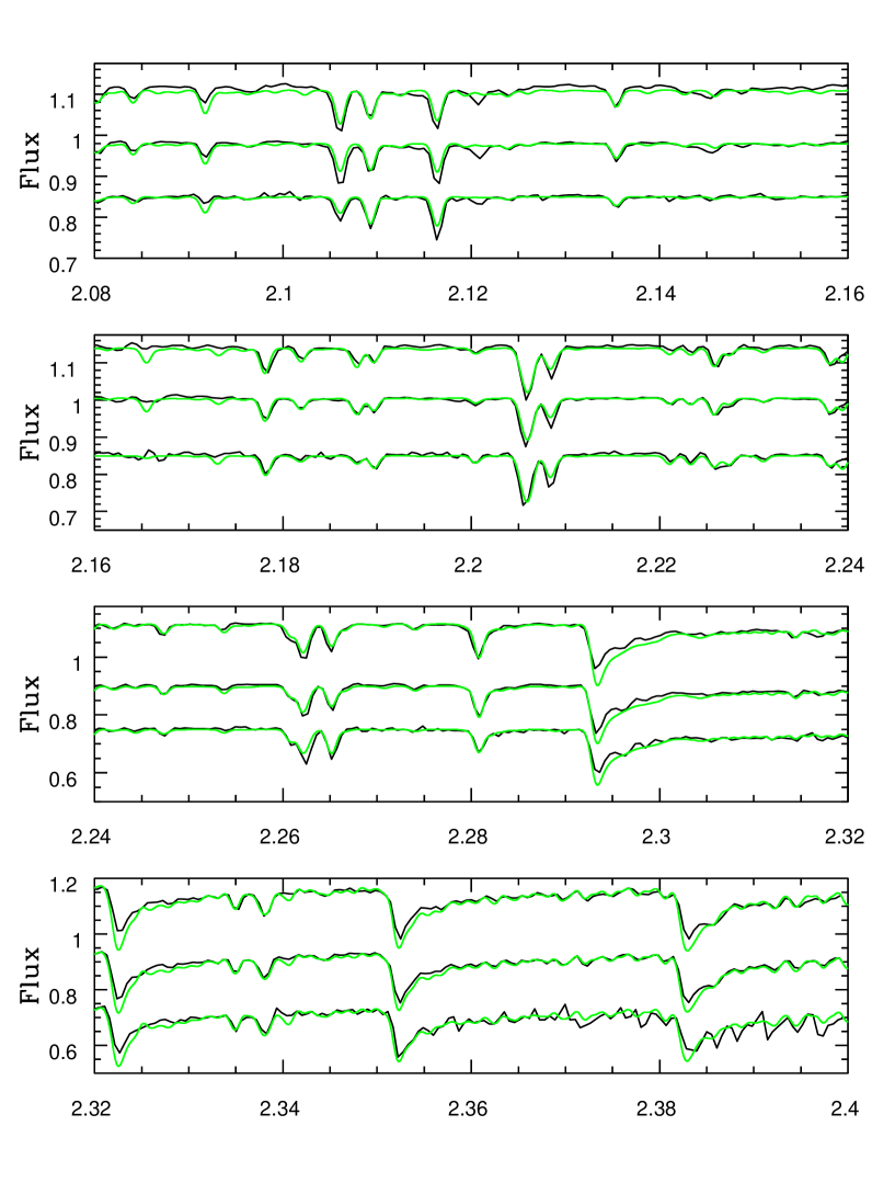
Figure 4: The SPEX spectra for K dwarfs spanning the spectral types from K4V to K7V (black), along with synthetic spectra (green) generated for each of the objects using the parameters listed in Table 2. For these stars, the model spectra are somewhat better at matching the observed spectra in the 2.10 to 2.15 $\mu$m region.

Given that the majority of CVs are too faint for moderate resolution infrared spectroscopy, most of the existing $K$-band data have been obtained at a lower resolution. To examine how well we can model such data sets we have downloaded SPEX data for dwarf stars spanning the spectral types K0V to K7V. The spectral type range K0V to K3V is shown in Fig. 3, while the range K4V to K7V is shown in Fig. 4. We generated synthetic spectra for each of these stars using the parameters listed in Table 2. The published metallicities produced excellent fits over most of the spectral range for all of the stars except HD145675 (K0V). We found that the best fitting model for HD145675 over the entire $K$-band required a lower metallicity, [Fe/H] = $+$0.25, than tabulated for this object (though within the observed error bars).

Close inspection of Fig. 3 shows that the synthetic spectra do not do a very good job of matching the strongest spectral features in the 2.10 to 2.15 $\mu$m bandpass. The origin of this discrepancy is not obvious. The fit of the synthetic spectra over the rest of the $K$-band suggests the tabulated (or derived) metallicities are correct. This might be a problem with continuum subtraction. To investigate this, we reduced and plot the SPEX data for the G9V star HD161198 observed during the same run as our program CVs [note that HD161198 is a spectroscopic binary with a cool secondary star (Duquennoy et al. 1996), and it is not a useful spectral template]. The model for HD145675 does a good job at fitting the spectrum of HD161198 in this range, indicating that continuum subtraction is not the issue. This suggests that the problem could be due to either the data reduction process, or some issue with the telluric standard and/or object spectra. The maximum amount of observed signal occurs in this bandpass, and the K0V, K1V, and K3V have $K$ $\leq$ 4.7 (HD3765 has $K$ = 5.16, while HD145675 has $K$ = 5.55), so perhaps it is a linearity issue. The discrepancy between the models and observed spectra in the 2.10 to 2.15 $\mu$m bandpass is not as severe for the K4V to K7V templates (even though the K7V template is 61 Cyg B, with $K$ = 2.32).

Clearly, however, our synthetic spectra do an excellent job at matching objects with known temperatures and metallicities. Especially important for the current program is the match of the model spectra to the observed CO features over a wide range of temperature and metallicity.

3.5 Creation of a Large Parameter Grid

In the preceding we have modeled the spectra of objects with known parameters. For modeling the CVs, where the temperatures and metallicities are poorly known, requires the generation of a large number of models, and a robust method to match the synthetic spectra to the observations. With the Python wrapper we have constructed to the modified version of the MOOG program described above, we are able to generate a large grid of models covering a user-defined range of the following parameters: T_eff, log $g$, [Fe/H], and [C/Fe]. Microturbulence was fixed at 2 km s^-1, and macroturbulence was not included since it is a small effect at the resolution of our observational data. In kmoog, if the synthetic spectra are designated to be stored as FITS files, each model actually contains two synthetic spectra: one unsmoothed, full resolution model, and one model convolved with a rotationally broadened spectrum appropriate for the target at the observed spectral resolution (which must be specified before the grid creation). A full grid covering the entire parameter space (3800 $\leq$ T_eff $\leq$ 5200 K, 3.0 $\leq$ log $g$ $\leq$ 5.0, $-1$ $\leq$ [Fe/H] $\leq$ $+$1, and $-1$ $\leq$ [C/Fe] $\leq$ $+$1) requires about one day to create on a 32 core machine and occupies $\sim$ 86 GByte in FITS output format. Obviously, smaller grids can be generated much more rapidly if the input parameter space can be narrowed.

3.6 Searching the Grid: Brute Force and Genetic Algorithms

With such large grids, it is easy to be overwhelmed by the quantity of data. Given a suitable subset of parameters, a direct grid search is possible; gather a list of valid models, and step through them one at a time comparing the model to observations. Given the sometimes low S/N of the observational data, however, a $\chi^{2}$ statistic is not calculated across the entire observational range, but restricted to the areas of greatest impact. For example, including Na I, Ca I, Mg I, Al I, Fe I lines, and the CO bands. This restricted region has the advantage of avoiding areas prone to increased levels of noise, and generally improves the quality of the fits to the observations.

Another method of stepping through the parameter space involves the use of an evolutionary algorithm to find the best fit to the data. Evolutionary algorithms are based off the ideas of biological evolution, the simple premise that in some given population only the “fittest individuals” (combination of all parameters) will “breed” and influence the next generation of that population. If we imagine representing our parameters as 1D binary strings, then the behavior and the manipulation of the binary strings over the course of the fit is not unlike that of DNA during reproduction. Sets of parameters can be mutated, introducing diversity into the population which helps to avoid getting stuck in a local maximum or minimum in the “$\chi^{\rm 2}$ landscape”. Mutations take the form of bit flips or swaps, analogous to transcription errors in DNA replication. We used a genetic algorithm framework called $PyEvolve$.

The algorithm proceeds as follows:

1. Make an initial first guess at the parameters based on spectral shape

2. Choose an appropriate maximum number of generations to evolve through as well as the initial population size

3. “Breed” and “mutate” the “fittest” members in the population to create a new generation

4. Repeat #3 until the population converges to the desired level

In this manner, all parameters are varied continually as the population converges towards some minimum $\chi^{2}$, at least a factor of four faster than the plain grid searching technique. Using both grid search and genetic algorithm techniques, the grid created with MOOG can be readily compared with the appropriate subset of CV spectra to attempt to determine as many stellar parameters as possible. Both methods are available in kmoog, though we find the brute force is sufficiently rapid and as reliable as the genetic algorithm technique. Heat maps showing the best fitting models for any two parameters are then generated to allow the determination of the best fitting model(s).

As we will find below, determining the exact value T_eff or [Fe/H] for an unconstrained object from a $K$-band spectrum is difficult. Many of the relevant oscillator strengths for transitions in this bandpass are unknown, and we have had to estimate a number of them by comparison of models to observations. In addition, our line list is incomplete, and thus weaker spectra features can contribute in a negative fashion to the assessment of the fit of a model to the data. The issues of telluric correction and continuum subtraction, as noted above, can introduce additional uncertainties into the goal of finding the best fitting solution. Thus, the $\chi^{2}$ analysis just described must be done carefully, focussing on the strongest spectral features, insuring that there is not a spectroscopic anomaly in that feature which can be attributed to random noise variation, or to the telluric correction process. It is extremely difficult to produce a fully automated best fit regimen that can blindly solve for the parameters of a previously unconstrained object in the $K$-band, even when focused on specific spectral lines. Currently, we manually examine the $\chi^{2}$ analysis for each line/region to insure that it is reliable, and that no unexpected events have occurred that affect the line/region under analysis. One such anomaly will be encountered shortly when we discuss the Al I line (at 2.116 $\mu$m) in SS Cyg. It has an unusual strength that defies obvious explanation. $\chi^{\rm 2}$ analysis of this line results in a super-solar abundance. We continue to work on the matching aspects of kmoog, but in its current state, a more interactive (“hands-on”) approach is required to insure the most robust results.

4 Results

Given that we have some information on the spectral types of the secondary stars in our CVs, we decided to use smaller grid than can be generated with the default settings of kmoog. For example, tests in Hamilton (2013) show that even the moderate resolution $K$-band spectra are inadequate for assessing gravity. Given the large rotational broadening of our targets, it will be impossible to constrain the surface gravity for the program CVs. Thus we fixed log $g$ = 4.5 for modeling SS Cyg and RU Peg, and log $g$ = 4.0 for GK Per (see below), to reduce parameter space, and increase the efficiency of the grid searching process. We postpone the discussion of error bar estimation to section 4.4.

4.1 SS Cyg

SS Cyg is the prototype long period (P_orb = 6.603 hr) dwarf nova with eruptions that recur on a monthly basis. Harrison et al. (2004) estimate the spectral type of the secondary as K4/K5, consistent with other published values. They noted, however, that the CO features were very weak for this spectral classification. Bitner et al. (2007) have used moderate resolution visual band spectroscopy to examine the masses of both components, and found that the secondary star is 10 to 50% larger than a star of its mass and temperature should be. They suggest that the secondary star in SS Cyg is evolved, and may have a core that is depleted in hydrogen. They also measured a rotational velocity of $v_{\rm rot}$sin$i$ = 89 km s^-1 for the secondary star.

The NIRSPEC spectrum of SS Cyg is presented in Fig. 5. The large rotational broadening of the spectral features is apparent. Our observations spanned $\Delta\phi$ = 0.05. At the observed phase (using the K₂ = 162.5 km s^-1 value derived by Bitner et al.), the total change in radial velocity over our set of observations would be $\Delta v$ = 11 km s^-1, resulting in minimal “orbital smearing.” Concentrating on the sixth order bandpass (2.095 to 2.128 $\mu$m), we convolved solar metallicity models having T = 4700 K with rotational velocities ranging from 70 to 110 km s^-1. The lowest $\chi^{\rm 2}$ values were for $v_{\rm rot}$sin$i$ = 90 $\pm$ 10 km s^-1. For the modeling below, we adopt the Bitner et al. value of $v_{\rm rot}$sin$i$ = 89 km s^-1 for SS Cyg.

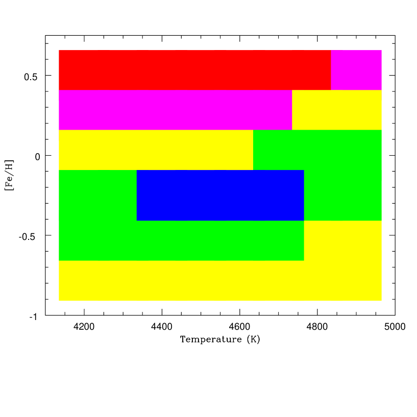
Figure 6: The $\chi^{2}$ heat map for the order 6 spectral region for the NIRSPEC spectrum of SS Cyg. In this, and all subsequent heat maps, blue denotes $\chi^{2}_{\rm red}$ $<$ 0.7, green is 0.7 $\leq$ $\chi^{2}_{\rm red}$ $<$ 0.9, yellow is 0.9 $\leq$ $\chi^{2}_{\rm red}$ $<$ 1.5, magenta is 1.5 $\leq$ $\chi^{2}_{\rm red}$ $<$ 2.5, and red is $\chi^{2}_{\rm red}$ $\geq$ 2.5.

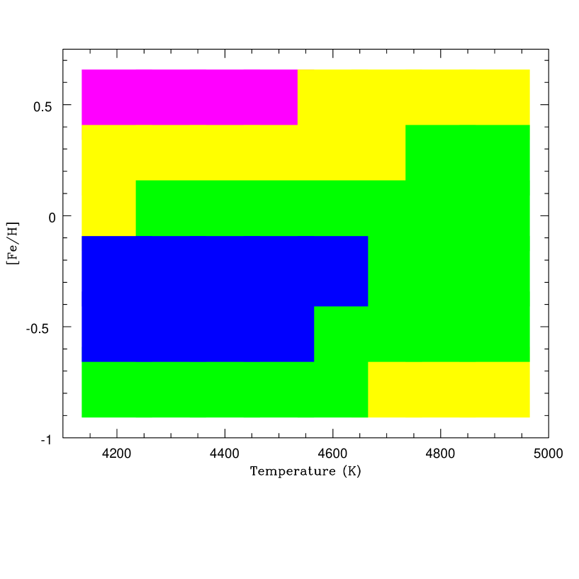
Figure 7: The $\chi^{2}$ heat map for the order 4 spectral region for the NIRSPEC spectrum of SS Cyg.

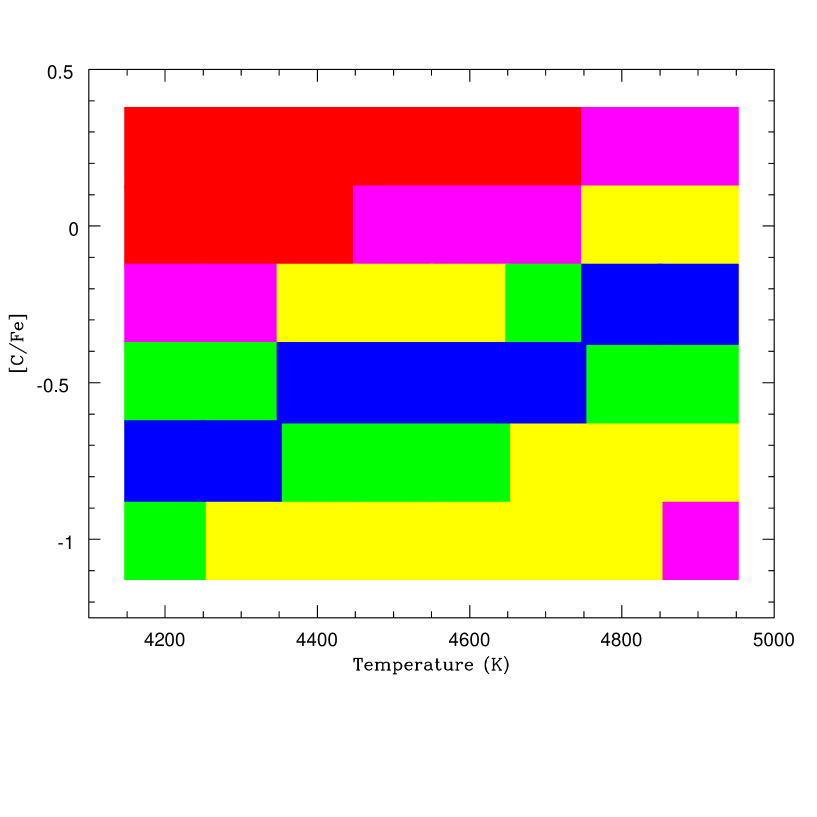
Figure 8: The $\chi^{2}$ heat map for the order 3 spectral region for the NIRSPEC spectrum of SS Cyg. For this analysis, a grid of models with the metallicity fixed to [Fe/H] = $-$0.25 was constructed, while the carbon abundance was altered over the range $-$1.0 $\leq$ [C/Fe] $\leq$ $+$0.25.

To attempt to reproduce the NIRSPEC data, we generated a grid of models spanning 4200 K $\leq$ T_eff $\leq$ 4900 K, $-0.75$ $\leq$ [Fe/H] $\leq$ $+$0.50, and $-1.00$ $\leq$ [C/Fe] $\leq$ $+$0.25. The resulting heat map for the sixth order, based on $\chi^{\rm 2}$ fits to only the first two of the three strong lines in the wavelength interval 2.104 and 2.118 $\mu$m is shown in Fig. 6. The best fit occurs for T = 4700 K, and [Fe/H] = $-$0.25. The fourth order contains a number of metal lines from Ti I and Fe I, though this spectral region is noisier than the data at shorter wavelengths. The resulting heat map, Fig. 7, is consistent with the result for the sixth order, though the value of [Fe/H] is less constrained. The results for the third order containing the ¹²CO_(2,0) bandhead is shown in Fig. 8, and suggests [C/Fe] $\leq$ $-$0.5.

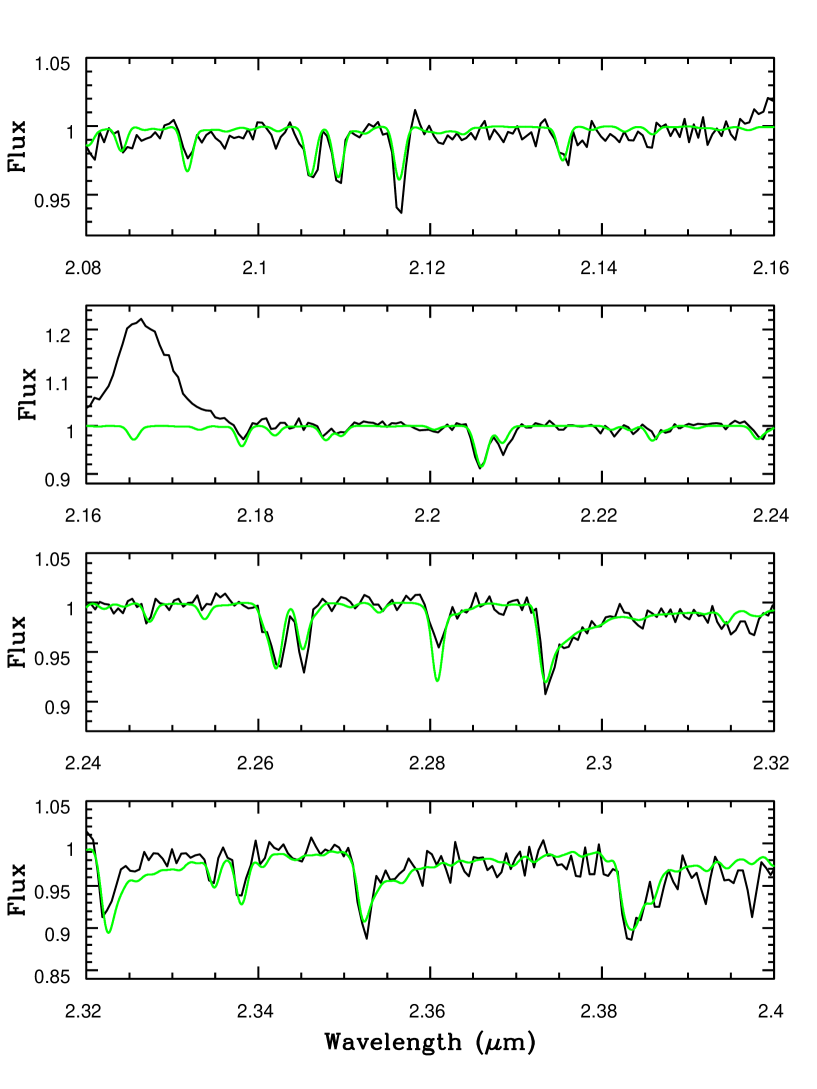
Figure 9: The lower resolution IRTF SPEX spectrum of SS Cyg covering the $K$-band from 2.08 $\mu$m to 2.4 $\mu$m with the best fit synthetic spectrum derived for the NIRSPEC data plotted in green. The S/N ratio at 2.20 $\mu$m was 115.

The best fit synthetic spectrum is overplotted on the data in Fig. 5 has these values, and fits the data set quite well. There is only one apparent anomaly in the NIRSPEC spectrum of SS Cyg, and that is the Al I line at 2.116 $\mu$m. We overplot the derived best fit model spectrum on the IRTF SPEX observation in Fig. 9. The fit is quite good, given the S/N of those data. The main differences between the model and the low resolution spectrum is again the Al I line 2.116 $\mu$m, and an Mg I feature at 2.282 $\mu$m. The Al I line was perfectly reproduced for the solar spectrum and for $\epsilon$ Eri, but does appear to be slightly under-predicted for the IRTF spectral sequence (though note our earlier discussion of the anomalous continuum in this bandpass). The line at 2.109 $\mu$m is also due to Al I, thus the abundance of aluminum is not unusual. It is odd that this line is perfectly reproduced for our other CVs. There is an He I line at this position that is often seen weakly in emission in the $K$-band spectra of other CVs with more prominent accretion disks, such as TT Ari, see Fig. 10. This emission line might be the cause of the peaks in the continuum on either side of this line in Fig. 9, but the effect of any such emission line would be to lessen the depth of the feature, not increase its strength.

The Mg I line at 2.282 $\mu$m is well reproduced by kmoog for all of the template star spectra. This line is very weak in the SPEX spectrum of SS Cyg. Since the Mg I line at 2.106 $\mu$m is at the appropriate strength in both the moderate and lower resolution data sets, we conclude that this is simply a S/N or telluric correction issue.

The NIRSPEC and SPEX data were obtained at quite different orbital phases, 0.20 and 0.40, respectively. The $K$-band light curve of SS Cyg presented in Harrison et al. (2007a) shows no evidence for irradiation at $\phi$ = 0.5, and the $K$ magnitudes at these two phases in this light curve are nearly identical. Thus, the fact that the same synthetic spectrum works for both epochs is not surprising. This does prove, however, that irradiation of the secondary star is not the source that weakens the CO absorption features, as the amount of the irradiated hemisphere seen at the dramatically different orbital phases of our spectra has no influence on the strength of the CO features.

4.2 RU Peg

RU Peg is a U Gem type dwarf nova of very long period (P_orb = 8.99 hr), whose binary parameters were first examined by Kraft (1962), observing doubled Ca II lines at some points in the orbital phase and a spectrum broadly consistent with a G8 IV to K0 V. Friend et al. (1990) observed the $\lambda$8190Å Na I doublet to measure radial velocity motion of RU Peg, finding that the secondary star is cooler and less massive than expected, with the spectrum being consistent with a K3 dwarf. They also note that the secondary star must be somewhat evolved, as the temperature, and masses derived are inconsistent with a main sequence dwarf. Harrison et al. (2004) presented IRTF observations of RU Peg, showing that the NIR spectrum was consistent with a spectral type of K2, but that RU Peg must contain a subgiant since it would be over-luminous for a dwarf at the distance given by its parallax. Dunford et al. (2012) recently presented spectra of RU Peg analyzed with Roche tomograms, deriving a much cooler spectral type of K5.

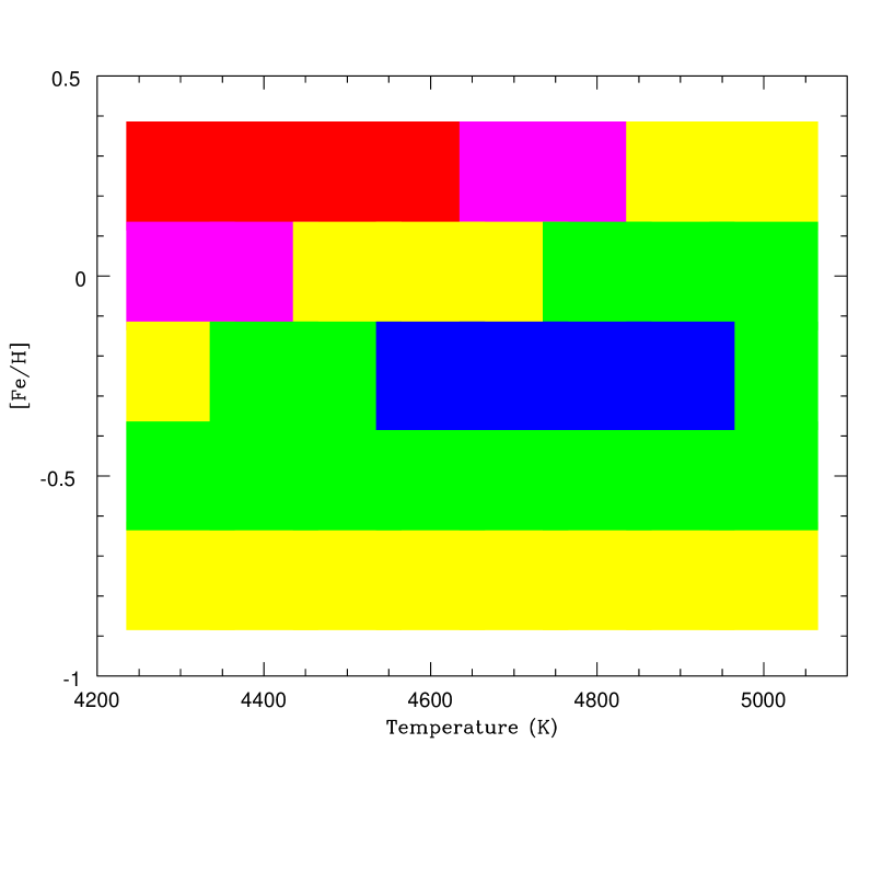
Figure 13: The $\chi^{\rm 2}$ heat map for the model grid fits to the fourth order spectrum of RU Peg.

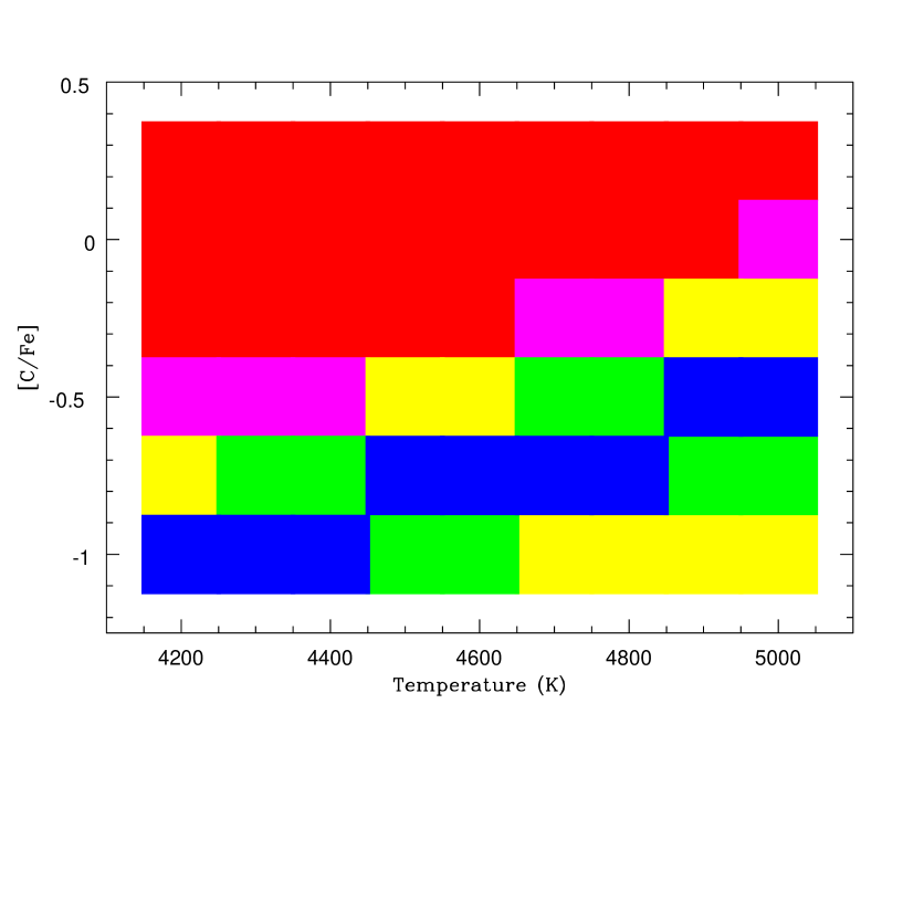
Figure 14: The $\chi^{\rm 2}$ heat map for the model grid fits to the third order spectrum of RU Peg. Like that for SS Cyg, a grid of single metallicity models (here with [Fe/H] = 0.0) were generated with only the carbon abundance altered for this analysis.

Along with the estimation of a cooler spectral type than found previously, Dunford et al. used moderate resolution visual band spectra to estimate $v_{\rm rot}$sin$i$ = 89 km s^-1. As for SS Cyg, we convolved a solar abundance model with T_eff = 4700 K to make our own estimate of the rotation velocity and found a slightly higher value of $v_{\rm rot}$sin$i$ = 95 $\pm$ 10 km s^-1. We have used this value in generating the synthetic spectra that follow. Using the same size grid as that for SS Cyg, the $\chi^{2}$ analysis for the sixth order, shown in Fig. 13, suggests solar metallicities, and 4600 $\leq$ T_eff $\leq$ 4700 K. The results for the fourth order (Fig. 12) indicate slightly subsolar metallicities, and 4500 $\leq$ T_eff $\leq$ 4900 K. We conclude that the secondary star has T_eff = 4700 K, and [Fe/H] = 0.0. Analysis of the CO features in the third spectral order (Fig. 14) finds [C/Fe] = $-$0.75.

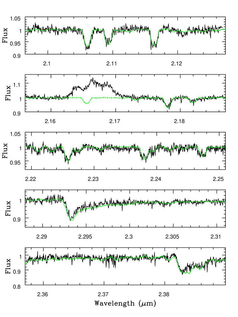
Figure 11: The NIRSPEC spectrum of RU Peg (black) with the best fit synthetic spectrum in green. The S/N ratio of these data ranged from 114 in the sixth order spectrum, to 69 in the second order spectrum.

A synthetic spectrum with these values is overplotted on the NIRSPEC data in Fig. 11, and provides an excellent fit to the data in all of the spectral orders. The H I emission from the disk is lower than seen in SS Cyg, and the underlying H I Br$\gamma$ absorption from the secondary star leaves its imprint on the emission line profile. Note that the long period and orbital phase at which the observations occurred make for minimal orbital smearing for the duration of our data taking: $\Delta v$ = 20 km s^-1.

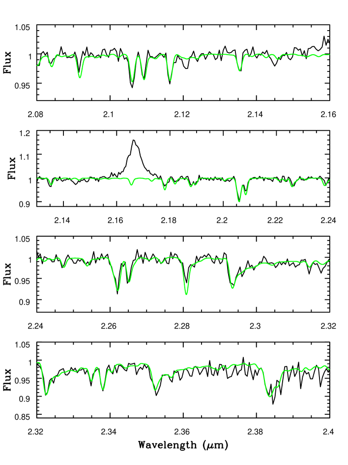
Figure 15: The SPEX spectrum of RU Peg (black) with the best fit synthetic spectrum plotted in green. The S/N ratio at 2.20 $\mu$m was 114.

The final model derived for the NIRSPEC spectrum is overplotted on the SPEX data in Fig. 15. This model fits the lower resolution data very well, including all of the other strong ¹²CO bandheads in the red part of the $K$-band. Sion et al. (2004) found that the carbon abundance in the photosphere of the white dwarf was 10% of solar. Thus, the carbon deficit observed in the UV can be directly traced to the secondary star. Sion et al. also found that silicon suffered a similar deficit as that of carbon. The most prominent Si I lines in the wavelength range plotted in Fig. 15 are at 2.136 and 2.189 $\mu$m, and while these lines are weak in our data, and the S/N not very high, they seem to be well represented by our solar abundance model.

4.3 GK Per

GK Per is an old classical nova, having experienced an extremely luminous nova eruption in 1901 (see Harrison et al. 2013). It has since exhibited periodic dwarf nova outbursts every 2-3 years since 1966, brightening by $\sim$ 3 mag during these events. Kraft (1964) detected the mass donor star in the optical, adopting a spectral type of K2 IV and noting that the spectrum was highly variable with an equivalent width of Sr II 4077 Å consistent with a giant at one point and a dwarf the next. More recently, Morales-Reuda et al. (2012) analyzed spectra of GK Per, finding that the donor star appeared as K1 IV. Their analysis consisted of an iterative template subtraction method, however, not direct detection of the secondary star. Harrison et al. (2007b) presented a $K$-band spectrum of the mass donor star in GK Per, and found that it has extremely weak CO features.

The radial velocity study conducted by Morales-Reuda et al. found $v_{\rm rot}$sin$i$ = 61.5 $\pm$ 11.8 km s^-1, K₂ = 120.5 $\pm$ 0.7 km s^-1, and a mass ratio of $q$ = 0.55 $\pm$ 0.21. Given the luminosity of its classical nova eruption suggests a massive white dwarf. If this is true, the radial velocity solution implies a surface gravity for the secondary star of log $g$ $\leq$ 4. As noted above, it is not possible to constrain the surface gravity of the program objects given the limitations of our data set. Thus, in contrast to SS Cyg and RU Peg, we set the surface gravity to log $g$ = 4.0 for our modeling of GK Per (though this produced identical results to models with log $g$ = 4.5). As for the preceding two objects, we analyzed the rotational velocity apparent in our NIRSPEC data and find $v_{\rm rot}$sin$i$ = 55 $\pm$ 10 km s^-1, slightly lower than that derived by Morales-Rueda et al., but agreeing within the error bars of the two measurements. We use this value in all of our modeling.

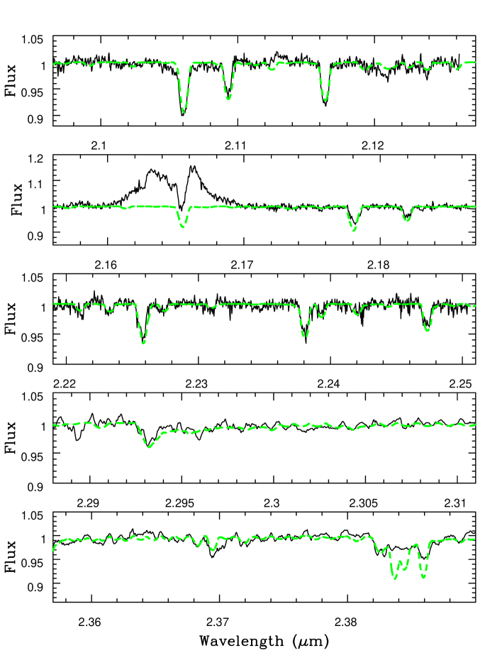
Figure 16: The NIRSPEC spectrum of GK Per (black). We have boxcar smoothed the second and third order spectra (by 9 pixels) to improve their S/N ratios. The final, best fit synthetic spectrum is plotted in green. The S/N ratio of these data ranged from 150 in the sixth order, to 50 in the second order.

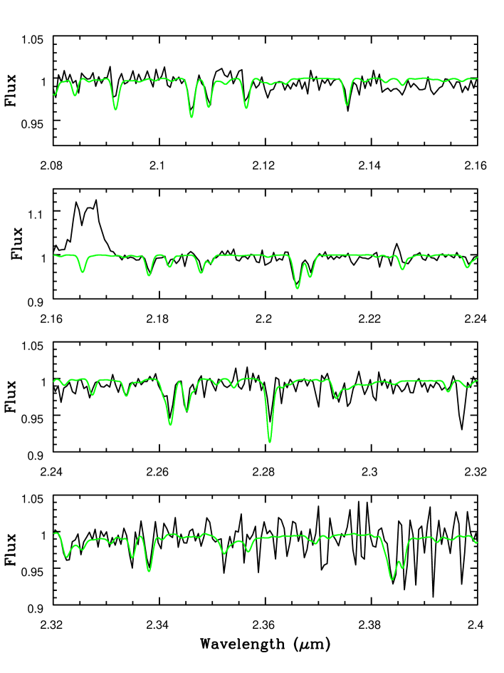
Figure 17: The SPEX spectrum of GK Per (black) with the best fit synthetic spectrum plotted in green. The S/N ratio at 2.20 $\mu$m was 91.

The NIRSPEC data is plotted in Fig. 16. $\chi^{\rm 2}$ analysis of the model grid found these best fit values: T_eff = 5100 K, [Fe/H] = $-$0.125, and [C/Fe] = $-$1.0. GK Per is fainter than our other two targets so the CO region is very noisy, and thus the measurement of [C/Fe] for GK Per is slightly less certain than found for the other two targets. It is interesting to note that the H I absorption of the underlying secondary star is sufficient to create the appearance of no H I Br$\gamma$ emission at the center of this feature. The SPEX spectrum of GK Per, Fig. 17, is even noisier than the NIRSPEC data. Clearly, however, the same model does an excellent job at fitting the observations.

4.4 Adopted Errors in Parameters

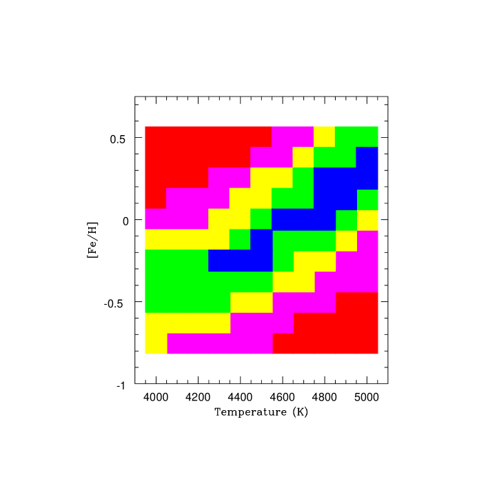
Figure 18: A heat map for the $\chi^{\rm 2}$ analysis of the IRTF spectral template HD36003 for a large grid of model spectra. The mean of the published values for this star, see Table 2, are T_eff = 4550 K, and [Fe/H] = $-$0.17. The grid has temperature intervals of 100 K, and [Fe/H] stepped by $\pm$0.125.

As demonstrated above, we are easily able to reproduce the spectra of objects with known parameters. Our examination of K stars in the IRTF spectral library shows that if we know the value of [Fe/H], we can derive values of T_eff, or vice versa, that are correct to within the published error bars for that object. To examine how well we can determine T_eff or [Fe/H] if we do not know either value, we present a $\chi^{\rm 2}$ analysis for the IRTF template HD36003. The heat map for the spectral region 2.18 $\leq$ $\lambda$ $\leq$ 2.37 $\mu$m of this star is shown in Fig. 18. While the models with parameters similar to the published values for both T_eff (4615 $\pm$ 29 K) and [Fe/H] ($-$0.14 $\pm$ 0.08) do have low values of $\chi^{\rm 2}$, there is a range of solutions with quantitatively similar fits to the data. As demonstrated in the plots shown in Figs. 3 and 4, for K dwarfs, the strong Na I doublet (at 2.209 $\mu$m), the Ca I triplet (at 2.26 $\mu$m), and the CO features all slowly get stronger as we decrease temperature. Thus, models can mimic the observed spectrum by either an enhanced abundance of [Fe/H] and a hotter temperature, or a reduced value of [Fe/H] and a lower temperature.

Our $\chi^{\rm 2}$ analysis over such a large span in wavelength is certainly also affected by missing transitions for weak lines, the S/N of the data, and for this lower resolution spectrum, the continuum subtraction process. The red end of the $K$-band is filled with strong telluric features, and even for high S/N data, small discrepancies can appear due to a slight mis-match of the telluric standard with the program object. This is especially clear for the CO features, as some bandheads in a particular spectrum are well fitted by the models, while others are not.

Given these results, if we are able to constrain the limits on the temperature of the object, such as “the secondary star in SS Cyg has a spectral type near K5”, and not expect super-solar metallicities, we find that temperatures derived from these data are good to $\pm$ 250 K, and [Fe/H] is good to $\pm$ 0.25. Moderate resolution data that covered either the Na I doublet or Ca I triplet would almost certainly lead to more precise values of both quantities.

Putting error bars on our values for [C/Fe] is more difficult in that none of our templates are known to have unusual values for this parameter. It is clear that our models reproduce the CO features in the template spectra over a large range in metallicity. Thus, altering just the abundance of carbon should not introduce any significant issues, as it simply acts to reduce the strength of the CO features to mimic those seen in lower metallicity stars. How a reduced carbon abundance affects the input stellar atmosphere is difficult to assess given the unknown evolutionary state of the CV secondary stars. The presence of more than one CO bandhead in all of the spectra also allows us to have more confidence in a particular value of [C/Fe]. For the higher S/N spectra, we expect that the precision of the values for [C/Fe] are similar in scale to [Fe/H]: $\pm$ 0.25. For GK Per the data are quite poor compared to the other two CVs, and the derived value for [C/Fe] is less certain. It is obvious, however, that the value of [C/Fe] is lower in GK Per than in the other two sources. This result will be amplified if the gravity of GK Per is significantly lower than our input value of log $g$ = 4.0.

5 Discussion

We have obtained moderate resolution $K$-band spectroscopy of three CVs that were previously noted to have weaker than expected CO features: SS Cyg, RU Peg, and GK Per. Because those earlier data were obtained at lower resolution, R $\sim$ 2,000, questions were raised about the possibility of “veiling” of the CO features to make them appear weaker. While we show below that this argument has no validity if realistic veiling scenarios are examined, it is the increased dispersion of the spectra obtained with NIRSPEC that easily argues against such a scenario. The NIRSPEC data have a dispersion of 0.32 Å/pix, nearly 1/17 that of the SPEX data. Thus, the flux per pixel from any veiling component would be diminished by this factor. Model spectra fitted to the two different sets of data would give different values for the strength of the CO features if there was some type of veiling confined to the CO region.

To provide quantitative estimates of the relative carbon abundances for CVs we have altered MOOG to allow us to model the entire $K$-band, and developed a software package that constructs large grids of synthetic spectra, and then searches these grids to find the best fitting solution to the observed data. We specifically allowed for the abundance of carbon to be a separate input under the assumption that the ¹²C abundance has been changed in the initial branches of the CNO cycle, as argued in Harrison et al. (2004). Obviously, weak CO features could be explained by a deficit of oxygen, but a process that could cause such a deficit is not obvious. With this software we derived values of T_eff, [Fe/H], and [C/Fe] from the NIRSPEC spectra for the three program objects. We list these results in Table 3. Except for the deficits of carbon, no other abundance anomalies are apparent, and the secondary stars of all three objects have solar, or slightly sub-solar abundances.

The total ¹²C abundance for SS Cyg and RU Peg are similar, $\sim$ 25% of solar, while for GK Per it is $\sim$ 10% of solar. If these peculiar values are the result of the CNO cycle (c.f., Marks & Sarna 1998), than the abundance of ¹³C should be enhanced, allowing for the detection of the bandheads of ¹³CO. The two strongest such bandheads with $\lambda<$ 2.4 $\mu$m are ¹³CO_(2,0) at 2.345 $\mu$m, and ¹³CO_(3,1) at 2.374 $\mu$m. The first of these is not covered by our NIRSPEC data, but Dhillon et al. (2002) present a $K$-band spectrum of SS Cyg which appears to show a strong ¹³CO_(2,0) absorption feature. They attribute this feature to metal line absorption in star spots as indicated by anomalously strong Na I absorption features (at 2.3355 and 2.3386 $\mu$m) in their spectra. These two Na I lines are not anomalous in our SPEX data, nor is there a ¹³CO_(2,0) feature of the strength observed by Dhillon et al. The second of the ¹³CO features is covered by our NIRSPEC observations, but there is a deep telluric feature at this wavelength that makes good correction quite difficult, and results in a noisy portion of the second order spectrum. Even with this issue, there is certainly no sign of a strong absorption feature at this location in either SS Cyg or RU Peg. The SPEX data covers both features, and while there are hints of both of these bandheads in the data for SS Cyg and RU Peg, the spectra are simply too noisy to draw any firm conclusions. New, higher S/N moderate resolution spectroscopy will be required to properly investigate the ¹²C/¹³C ratio.

5.1 A Closer Inspection of the Continuum of SS Cyg, and an Examination of Realistic Veiling Scenarios

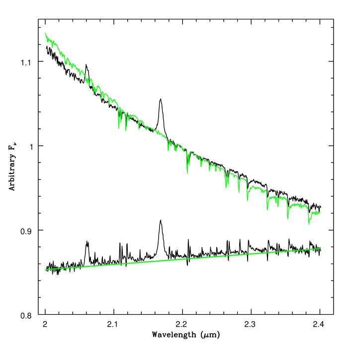
Figure 19: The SPEX spectra of SS Cyg (black) and the K4V template HD45977 (green) normalized at 2.2 $\mu$m. Subtraction of the spectrum of HD45977 from that of SS Cyg leaves the residual spectrum (bottom) that has a flat slope (f_ν $\propto$ $\nu^{\rm-0.16}$).

Harrison et al. (2004) found that the $K$-band continua of many long period CVs were flatter than expected if the secondary star was the sole source of emission in that bandpass. To more closely examine the slope of the continuum of SS Cyg, we compare the full $K$-band spectrum of SS Cyg with that of the IRTF template star that has the most similar temperature: HD45977. In Fig. 19, we subtract the spectrum of HD45977 from that of SS Cyg, both spectra having been normalized at 2.2 $\mu$m. The result is a residual spectrum that is fairly flat, with f_ν $\propto$ $\nu^{\rm-0.16}$. Given the uncertainties in the temperatures of the two objects, and the differing sources of the data, such a flat spectrum is consistent with free-free emission. The continuum subtraction process step required to allow us to directly compare the SPEX data to the synthetic spectra easily removes a weak continuum source such as this, and this is why the results for the NIRSPEC and SPEX are simultaneously consistent with the same model.

We can also attempt to model the contribution of line emission sources that might preferentially veil the CO features. There are only two possible sources that we can envision that might do this: the H I Pfund continuum, and CO emission. As shown in Fig. 19, the H I Br$\gamma$ emission line in SS Cyg is quite strong, so the Pfund series of hydrogen will also be present. The Pfund series limit is at $\lambda$2.279 $\mu$m, and the transitions Pf23 and higher, will fall in our modeling bandpass. The emissivities of these lines are very small; Hummer & Storey (1987) list them as being $\leq$ 1.7% that of Br$\gamma$ (for “Case B” conditions). Fitting the Br$\gamma$ line with a Gaussian profile gives FWHM = 73 Å. We will assume all of the H I lines have this profile. In Fig. 20, we present spectra where we added a rotationally broadened spectrum of the Pfund series (up to Pf100) to the K4V spectral template, and compare it to the spectrum of SS Cyg. Given their low emissivities, the effect of the H I lines is not detectable. We also artificially multiplied the emissivities of the Pfund lines by factors 10 and 100 and added them to the K4V template. Only at very large multiplicative factors can their presence be detected, and even then, they add a smooth continuum to the CO region, leaving the absorption features relatively undisturbed, but producing a highly distorted continuum. Even with this simplistic model, it is clear that H I Pfund emission cannot provide the veiling necessary to explain weak CO features.

The detection of CO emission in WZ Sge (Howell et al. 2004) has led to the suggestion that CO emission is the source of the veiling needed to produce weaker than expected CO features seen in the program CVs. Since the CO emission must come from the accretion disk, a similar result as that for the Pfund continuum emission attains. As discussed in Scoville et al. (1980), such emission is expected to be confined to regions where T $>$ 3000 K, and where the densities are high, $n_{\rm e}$ $\geq$ 10¹⁰ cm^-3. Since SS Cyg was in a minimum during our observations, presumably these conditions exist somewhere within its accretion disk. As shown in Bik et al. (2006), optically thin CO emission features are essentially the inverse of the CO absorption features seen in late type stars. This similarity allows us to construct crude models to investigate what CO emission might look like if its origin was in a CV accretion disk.

If we assign the CO emission to the disk, then the broadening of any spectral feature located there will be much greater than that of the slower rotational broadening of the secondary star (89 km s^-1 in the case of SS Cyg). For example, if the accretion disk extends to 75% of R${}_{\rm L_{\rm 1}}$ (the Roche lobe radius of the white dwarf), using the stellar parameters for SS Cyg in Bitner et al. (2007), the Keplerian velocity at this radius will be $\sim$ 400 km s^-1. In Fig. 21, we add a rotationally broadened CO spectrum to the best fitting synthetic spectrum for SS Cyg using the value for the H I Br$\gamma$ line (FWHM = 73 Å), and a CO emission spectrum broadened by half that value. As could be expected, the result is a dramatic change in the profiles of the CO features, with an emission peak preceding each bandhead, a subtle redward shift for the location of the strongest absorption, and a dramatic narrowing of the CO bandhead profiles. Obviously, the data for none of our objects resembles this result. More complicated scenarios for the emission profile could be constructed, but to truly diminish the CO features without distorting the resulting spectrum requires the addition of CO emission with a broadening profile that is very similar to that of the secondary star. There is no other location in a CV system besides the secondary star photosphere where such low velocities occur.

6 Conclusions

We have modified the spectral synthesis program MOOG and have demonstrated that we are able to model moderate and lower resolution $K$-band spectra for stars hotter than T_eff $\geq$ 4000 K. We then used this program to investigate such spectra for three CVs: SS Cyg, RU Peg, and GK Per. It is clear that all three CVs in this sample have subsolar carbon abundances. That synthetic spectra with identical parameters simultaneously model data with dramatically different dispersions for each of the objects, and realistic CO veiling scenarios fail to reproduce the observed CO features, proves that the carbon deficits are real. It is important to note that these results represent the first direct measurements of abundances in the photosphere of the mass donor stars in CVs. While our determinations of T_eff, [Fe/H], and [C/Fe] for these three objects are not overly precise, they have no parallel. There have not been many predictions for the behavior of the abundances in the atmospheres of CV donor stars as a function of age/evolutionary state. Marks & Sarna (1998) explored how the photospheric abundances of CNO elements in CV secondaries might evolve with time, including the possibilities of pollution by the common envelope phase, or through the accretion of classical novae ejecta. They found that the latter two scenarios were inadequate in producing observable changes, and concluded that only pre-contact evolution could significantly alter the CNO abundances and isotopic ratios in CV secondary star photospheres. Schenker et al. (2002) examined how CVs might evolve from supersoft binaries and, if so, could show dramatic changes in CNO species. In light of our results, it would be useful to revisit this research with newer generations of binary star evolution codes, such as STAREVOL (Stancliffe & Eldridge 2009). It is also obvious that moderate resolution spectroscopy of the brightest CVs covering the entire $K$-band are required to achieve more robust measures of [Fe/H], as well as allow for the proper examination of the CO bands. If the deficits of carbon arise from the CNO cycle, than the isotopic abundances of carbon will be altered. Moderate resolution $K$-band spectroscopy covering the main ¹³CO features will allow for the confirmation of this inference.

Table 1: Observation Log

Object	Instrument	Date	Start Time	#Exp. $\times$ Integration	Orbital Phase
			(UT)	Time (s)
SS Cyg	NIRSPEC	2004 Aug. 28	12:31:51	4 $\times$ 300	0.20
RU Peg	NIRSPEC	”	13:17:12	4 $\times$ 300	0.87
GK Per	NIRSPEC	”	14:20:24	6 $\times$ 300	0.46
$\gamma$ Psc	NIRSPEC	”	13:45:17	8 $\times$ 1	$\cdots$
$\epsilon$ Eri	NIRSPEC	”	15:06:18	24 $\times$ 1	$\cdots$
SS Cyg	SPEX	2004 Aug. 15	08:55:17	8 $\times$ 180	0.40
RU Peg	SPEX	”	10:25:06	8 $\times$ 240	0.85
GK Per	SPEX	”	13:53:54	6 $\times$ 240	0.94

Table 2: Spectral Template Objects

Object	Spectral Type	Temperature (K)	log(g)	[Fe/H]	# of Measures
Sun	G2V	5777	4.44	0.0	$\cdots$
Arcturus	K0III	4313 $\pm$ 84	1.65 $\pm$ 0.30	$-$0.54 $\pm$ 0.10	34/31/31
$\epsilon$ Eri	K2V	5088 $\pm$ 72	4.54 $\pm$ 0.16	$-$0.09 $\pm$ 0.09	26/24/24
$\gamma$ Psc	G9III	4853 $\pm$ 45	2.59 $\pm$ 0.26	$-$0.46 $\pm$ 0.12	11/8/8
HD145675	K0V	5320 $\pm$ 114	4.45 $\pm$ 0.07	$+$0.41 $\pm$ 0.12	18/15/15
HD10476	K1V	5189 $\pm$ 53	4.46 $\pm$ 0.12	$-$0.06 $\pm$ 0.06	16/10/10
HD3765	K2V	5023 $\pm$ 66	4.53 $\pm$ 0.16	$+$0.05 $\pm$ 0.10	7/4/4
HD219134	K3V	4837 $\pm$ 138	4.51 $\pm$ 0.13	$+$0.05 $\pm$ 0.10	15/10/10
HD45977	K4V	4689 $\pm$ 174	4.30 $\pm$ 0.39	$+$0.03 $\pm$ 0.18	1/1/1
HD36003	K5V	4615 $\pm$ 29	4.35 $\pm$ 0.06	$-$0.14 $\pm$ 0.08	3/2/2
HD201092	K7V	3964 $\pm$ 175	4.50 $\pm$ 0.18	$-$0.26 $\pm$ 0.27	10/5/5

Table 3: Derived Secondary Star Parameters

System	$T_{\mathrm{eff}}$ (K)	log $g$	$\left[Fe/H\right]$	$\left[C/Fe\right]$
SS Cyg	4700 $\pm$ 250	4.50	$-$0.25 $\pm$ 0.25	$-$0.50 $\pm$ 0.25
RU Peg	4700 $\pm$ 250	4.50	$+$0.00 $\pm$ 0.25	$-$0.75 $\pm$ 0.25
GK Per	5100 $\pm$ 250	4.00	$-$0.125 $\pm$ 0.25	$-$1.00 $\pm$ 0.50

Figure 10: The IRTF SPEX $K$-band spectrum of TT Ari, obtained on 2004 August 15. This disk dominated system has a weak He I emission feature at 2.11 $\mu$m.

Figure 12: The $\chi^{\rm 2}$ heat map for the model grid fits to the sixth order spectrum of RU Peg.

Figure 20: The SPEX spectrum of SS Cyg (top). The next spectrum down is a synthetic spectrum for a solar abundance K4V to which we have we have added a Gaussian broadened H I emission line spectrum to match the profile and strength of the H I Br $\gamma$ line of SS Cyg. The spectrum below that has had the emissivities of the Pfund lines increased by a factor of 10. The bottom spectrum has the Pfund line emissivity increased by a factor of 100.

Figure 21: The SPEX spectrum of SS Cyg (middle). The top spectrum results from the addition of a CO emission line spectrum Gaussian broadened to match the Br $\gamma$ line, added to the best fitting (solar abundance) synthetic spectrum. The bottom spectrum is the result of the identical process, except the velocity broadening was one half that of Br $\gamma$ profile. The CO emission component was normalized so that when it was added to the model spectrum, the depth of the minima in the CO features of SS Cyg were reproduced. Dashed vertical lines indicate the wavelengths of the ¹²CO_(2,0) (left) and ¹²CO_(3,1) (right) bandheads.