A Perturbative Analysis of Synchrotron Spectral Index Variation over Microwave Sky

Abstract

In this paper, we implement a perturbative approach, first proposed by Bouchet & Gispert (1999), to estimate variation of spectral index of galactic polarized synchrotron emission, using linear combination of simulated Stokes Q polarization maps of selected frequency bands from WMAP and Planck observations on a region of sky dominated by the synchrotron Stokes Q signal. We find that, a first order perturbative analysis recovers input spectral index map well. Along with the spectral index variation map our method provides a fixed reference index, $\hat{\beta}_{0s}$, over the sky portion being analyzed. Using Monte Carlo simulations we find that, $\langle\hat{\beta}_{0s}\rangle=-2.84\pm 0.01$, which matches very closely with position of a peak at $\beta_{s}(p)=-2.85$, of empirical probability density function of input synchrotron indices, obtained from the same sky region. For thermal dust, mean recovered spectral index, $\langle\hat{\beta}_{d}\rangle=2.00\pm 0.004$, from simulations, matches very well with spatially fixed input thermal dust spectral index $\beta_{d}=2.00$. As accompanying results of the method we also reconstruct CMB, thermal dust and a synchrotron template component with fixed spectral indices over the entire sky region. We use full pixel-pixel noise covariance matrices of all frequency bands, estimated from the sky region being analyzed, to obtain reference spectral indices for synchrotron and thermal dust, spectral index variation map, CMB map, thermal dust and synchrotron template components. The perturbative technique as implemented in this work has the interesting property that it can build a model to describe the data with an arbitrary but enough degree of accuracy (and precession) as allowed by the data. We argue that, our method of reference spectral index determination, CMB map, thermal dust and synchrotron template component reconstruction is a maximum likelihood method.

1. Introduction

Observations of microwave signal by WMAP and Planck satellite missions, in the frequency range $23$ GHz to $857$ GHz, can be used to obtain a wealth of precise cosmological information (e.g, precise values of basic cosmological parameters (Hinshaw et al., 2013; Bennett et al., 2013; Planck Collaboration et al., 2015c), topology of space (Planck Collaboration et al., 2015f), laws and nature of physical conditions existing at different epoch marked by different phases of dynamical evolution of space-time  (Planck Collaboration et al., 2015g, e, 2014, d)) as well as precise information about various astrophysical mechanisms operating since recent times that cause diffuse emissions inside Milky Way (Bennett et al., 2003; Planck Collaboration et al., 2015h, 2013; Dobler, 2012). However, extracting these information accurately with precision requires a method that separates different components from their observed mixture using a model that is flexible enough to describe the data with an arbitrary but desired degree of minute closeness as permissible by data. A completely accurate model may produce ambiguous results if the data is simply insufficient to constrain all model parameters correctly e.g., consider the astrophysical problem of reconstruction various galactic emission components which is a greatly complex task due to inherent degeneracy existing in the morphological pattern of these emissions, degeneracy arising due to similarities in physical models of multiple emissions or due to other reasons. Such uncertainties in reconstructed foreground components may cause cosmological inferences drawn from the analysis of reconstructed Cosmic Microwave Background (CMB) maps to be biased (Tegmark et al., 2000) if these uncertainties are not known or if they are not properly taken into account.

One of the prime source of uncertainties against properly extracting the primordial signal and other galactic foreground components from observed maps is intrinsic variation of spectral index of synchrotron emission (Tegmark, 1998) over the sky due to variations of number density of cosmic ray electrons in our galaxy. In this paper we implement a novel method on simulated WMAP and Planck Stokes Q frequency maps to perturbatively model the synchrotron spectral index variation over the sky following the approach proposed by Bouchet & Gispert (1999). The perturbative nature of the method is very desirable since it allows one to build a model with just enough accuracy that is still meaningful within the available data. As associated results of the method we reconstruct best-fit map for CMB and templates for thermal dust and synchrotron emission.

Usefulness of the method described in this paper can also be seen from a different perspective. There exist several methods in the literature for CMB or (and) foreground component reconstruction which can be grouped broadly in following three categories:

1. The so-called blind, internal-linear-combination approach, ((Tegmark & Efstathiou, 1996; Maino et al., 2002; Tegmark et al., 2003; Delabrouille et al., 2009; Saha, 2011; Bennett, 2012; Planck Collaboration et al., 2015a)), where one removes foregrounds based upon the fact that CMB follows blackbody spectrum whereas, other components do not. In principle, this method can also be used to produce a cleaned map of any of the foreground components (Remazeilles et al. (2011)), provided its spectral index is a priori known and is constant over the sky portion being analyzed. The method by definition is a non-Maximal Likelihood (ML) approach since it incorporates minimum information about the physical components and no information about detector noise.

2. The second class (Eriksen et al. (2008a, b); Planck Collaboration et al. (2015b, a)) is that one where one uses as much prior information as possible about all components, along with the detector noise model, to perform a ML analysis of the data. The outcome of this method are ML estimates of all components.

3. The third one is an intermediate approach of the first and second categories. Although, here one incorporates informations about various components available from prior observations, (e.g., Maximum Entropy Method, (Hobson et al., 1998; Bennett et al., 2003; Hinshaw et al., 2007; Gold et al., 2009, 2011)  and the Wiener filtering approach, (Bunn et al., 1994; Tegmark & Efstathiou, 1996; Bouchet et al., 1999)), it is a non ML approach.

All the above methods have merit and demerit of their own. ML approach has advantages that it is the optimal method in the sense that it retains all information of the data and provides maximum precision on the derived parameters. ML method may, however, be biased if the model to be used for the data is not accurately known, or, if there are degeneracies between the parameters. The non-ML approaches are advantageous since data is processed with the minimal assumptions. However, it is a sub-optimal method and can be biased. One, therefore, desires to ask a question can we develop a method which requires minimal assumptions in terms of data model (e.g., no requirement of using templates) and, at the same time, which is a ML approach with respect to at the least almost all of its parameters? So far, there has not been any attempt in the literature to answer this question. The novel perturbative approach for component separation and for determination of variation of spectral index of synchrotron emission followed in this paper, at one-side, is a linear-combination method, on the other side, is a ML approach with respect to all of its component templates and best-fit spectral indices for synchrotron and thermal dust. The method incorporates information about spectral properties of components and detector noise model, thus preserving properties of first and second categories described above.

There have many attempts in the literature to measure synchrotron spectral index of our Galaxy. Reich & Reich (1988) find map of synchrotron spectral index between $420$ MHz and $1420$ MHz using radio continuum surveys. Following the method of TT plot Davies et al. (1996) find synchrotron temperature spectral index lies in the range $-2.8$ to $-3.2$ from a strip at $\delta=40^{\circ}$ latitude sections of $408$ MHz and $1420$ MHz maps. Platania et al. (1998) find synchrotron spectral index between $420$ MHz and $7.5$ GHz as $-2.76\pm 0.11$. Bennett et al. (2003) find a flatter synchrotron spectral index, $\sim-2.5$, near the galactic plane and a steeper index, $\sim-2.9$ towards the higher galactic latitude. Using WMAP nine-year data  Fuskeland et al. (2014) estimate polarized synchrotron spectral index towards galactic plane as $-2.98\pm 0.01$, and a steeper spectral index, $-3.12\pm 0.04$, towards the higher galactic latitude.

We present our paper as follows. We describe the problem in Section 2. In Section 3 we describe the perturbative approach used to model the data. We discuss basic formalism of this work in Section 4. Here we discuss 1) the power minimization algorithm (based upon the model described in Section 3) and how the power minimization algorithm leads to an equation for weights that we use for linear combination of input Stokes Q maps, later in Section 5, 2) the difference map at each frequency bands, and the noise covariance matrix thereof, 3) the $\chi^{2}$ data-model mismatch statistics and 4) relationship of our method with ML approaches. In Section 5 we describe the method used in this paper. We present results in Section 6. Finally, we conclude in Section 7.

2. Basic Problem

Let us assume we have observations of CMB and foreground polarizations at $n_{b}$ different frequency bands. Each frequency band contains contribution from $n$ different physical components, namely, CMB and emissions from $n-1$ foreground components - each with a given spectral index all over the sky - plus detector noise . If foreground component $j$ has a fixed spectral index, $\beta_{j}$, all over the sky, net polarized Stokes Q signal, $Q_{i}(p)$, at a pixel $p$, due to CMB, $Q_{c}(p)$, all foregrounds, $Q_{0j}$, and detector noise, $Q^{n}_{i}(p)$ at a frequency $\nu_{i}$ in thermodynamic temperature unit is given by,

$$Q_{i}(p)=Q_{c}(p)+\sum_{j=1}^{n-1}a_{i}\left(\frac{\nu_{i}}{\nu_{0j}}\right)^{\beta_{j}}Q_{0j}(p)+Q^{n}_{i}(p)\,,$$ (1)

where $a_{i}\equiv a(\nu_{i})$ denotes conversion factor from antenna to thermodynamic temperature unit at frequency $\nu_{i}$ for all foreground components. CMB anisotropy at any given pixel $p$ is independent on frequency $\nu_{i}$ due to its blackbody nature. Each foreground template $Q_{0j}$ is defined with reference to frequency $\nu_{0j}$, which may be different for different foreground components. We note that, in general, observed maps for different frequencies are convolved by different instrument response functions. However, we implicitly assume that frequency maps, $Q_{i}(p)$, in Eqn 1 already have been brought to a common resolution by properly deconvolving first by respective instrument response functions and then convolving again by the common response function. Since all frequency maps of our work are convolved by a common Gaussian beam function of FWHM = $20^{\circ}$ we omit reference to beam function in all equations of this paper containing frequency maps, CMB or foreground templates.

For polarized signal there are only two foreground components at microwave frequencies, namely, synchrotron and thermal dust. Moreover, the spectral index for synchrotron emission varies with sky position due to variation of relativistic electron density over the sky. In the presence of variation of spectral index for synchrotron, but fixed spectral index for thermal dust component Eqn 1 reduces to,

$$\begin{aligned} Q_{i}(p)={}&Q_{c}(p)+a_{i}\left(\frac{\nu_{i}}{\nu_{0s}}\right)^{\beta_{s}(p)}Q_{0s}(p)\\ &+a_{i}\left(\frac{\nu_{i}}{\nu_{0d}}\right)^{\beta_{d}}Q_{0d}(p)+Q^{n}_{i}(p)\,,\end{aligned}$$ (2)

where $\beta_{s}(p)$ represents the synchrotron spectral index at a pixel $p$ and $\beta_{d}$ is the global thermal dust spectral index. The motivation for our work is to obtain a reliable estimate of $\beta_{s}(p)$ using a perturbative analysis, without assuming any prior template models for foregrounds or CMB.

3. Perturbative Data Model

Let us consider a given region of sky. Synchrotron spectral index at a pixel $p$ can be written as, $\beta_{s}(p)=\beta_{0s}+\Delta\beta_{s}(p)$, where $\beta_{0s}$ represents some reference spectral index for the region and $\Delta\beta_{s}(p)$ represents actual variation of spectral index over $\beta_{0s}$ inside the region. Using the direction dependent spectral index, $\beta_{s}(p)$, in the second term of Eqn 2, one can show that (Bouchet & Gispert, 1999),

$$\left(\frac{\nu_{i}}{\nu_{0s}}\right)^{\beta_{s}(p)}=\left(\frac{\nu_{i}}{\nu_{0s}}\right)^{\beta_{0s}\left(1+\frac{\Delta\beta_{s}(p)}{\beta_{0s}}\right)}$$ (3)

$$\sim\left(\frac{\nu_{i}}{\nu_{0s}}\right)^{\beta_{0s}}\left(1+\Delta\beta_{s}(p)\ln\left(\frac{\nu_{i}}{\nu_{0s}}\right)\right)\,,$$

where the second line follows from Taylor expansion of the left hand side of above equation up to first order in $\Delta\beta_{s}(p)/\beta_{0s}$, assuming $\Delta\beta_{s}(p)/\beta_{0s}\ll 1$. Using Eqn. 3 in Eqn. 2 we obtain,

$$\begin{aligned} Q_{i}(p){}&{}=Q_{c}(p)+a_{i}\left(\frac{\nu_{i}}{\nu_{0s}}\right)^{\beta_{0s}}Q_{0s}(p)+a_{i}\left(\frac{\nu_{i}}{\nu_{0s}}\right)^{\beta_{0s}}\ln\left(\frac{\nu_{i}}{\nu_{0s}}\right)\\ &\times Q_{0s}(p)\Delta\beta_{s}(p)+a_{i}\left(\frac{\nu_{i}}{\nu_{0d}}\right)^{\beta_{d}}Q_{0d}(p)+Q^{n}_{i}(p)\,.\end{aligned}$$ (4)

Apart from CMB and detector noise, our data model given by above equation, can now be interpreted nicely to consist of a total of three foreground emission components, namely, synchrotron with a constant spectral index $\beta_{0s}$, a second component $Q_{0s}(p)\Delta\beta_{s}(p)$, with its frequency variation $a_{i}\left(\frac{\nu_{i}}{\nu_{0s}}\right)^{\beta_{0s}}\ln\left(\frac{\nu_{i}}{\nu_{0s}}\right)$ and finally thermal dust component. As we can see from above equation our model renders the variation of spectral index of synchrotron component in terms of a new foreground component with rigid frequency scaling. We define a set of templates, $T_{j}$, where $j\in\{1,2,3,4\}$ following,

$$\begin{aligned} &T_{1}(p)=Q_{c}(p)\\ &T_{2}(p)=Q_{0s}(p)\\ &T_{3}(p)=Q_{0s}(p)\Delta\beta_{s}(p)\\ &T_{4}(p)=Q_{d}(p)\,.\end{aligned}$$ (5)

With these definitions, total polarized emission of Eqn. 4, at a frequency $\nu_{i}$ is then given by,

$$Q_{i}(p)=\sum_{j=1}^{4}T_{j}(p)s^{j}_{i}+Q^{n}_{i}(p)\,,$$ (6)

where we have denoted emission from $j^{th}$ component at channel $i$ (in thermodynamic temperature unit) by $T_{j}(p)s^{j}_{i}$. $T_{j}(p)$ denotes template for $j^{th}$ component based on reference frequency $\nu_{0j}$ and $s^{j}_{i}$, for a given $j$, denotes elements of so-called shape vector, $[{\bf s}]_{j}$, for component $j$. For foregrounds with emissions following usual power law behavior elements of the shape vector are given by ,

$$s^{j}_{i}=\left(\frac{\nu_{i}}{\nu_{0j}}\right)^{\beta_{j}}a(\nu_{i})\,,$$ (7)

where $\beta_{j}$ represents spatially fixed spectral index of $j^{th}$ (foreground) component. Following method as described in Section 5 we reconstruct each template defined by Eqn 5. Due to presence of detector noise, the reconstructed templates, $\hat{T}_{j}(p)$, are, however, different from $T_{j}(p)$. Once all template components are reconstructed, synchrotron spectral index variation map is obtained following,

$$\Delta\hat{\beta}_{s}(p)=\hat{T}_{3}(p)/\hat{T}_{4}(p)\,.$$ (8)

4. Formalism

4.1. Component Reconstruction and Weights

From a mixture of $n$ physical components present in different frequency bands, our aim is to isolate best-fit map of each one of them by removing rest. This can be achieved by reconstructing any one component first and then repeating the method for all other components. Let us denote the component to be reconstructed by a Greek letter subscript, e.g., $\alpha$ and other components to be removed by any Roman letter subscript taking values from the difference set $\{1,2,...,n\}-\{\alpha\}$. We denote shape vector for the component to be reconstructed by $[{\bf s}]_{\alpha}$ while each of the rest $n-1$ components has shape vector $[{\bf s}]_{i}$. To reconstruct the cleaned template, $\hat{T}_{\alpha}(p)$, for component $\alpha$, we form a linear combination of available maps following,

$$\hat{T}_{\alpha}(p)=\sum_{i=1}^{n_{b}}w^{i}_{\alpha}Q_{i}(p)\,,$$ (9)

where the linear weights, $w^{i}_{\alpha}$, for $\alpha$ component is obtained by minimizing the total pixel-pixel variance, $\sigma^{2}_{\alpha}$, of the cleaned template, $\hat{T}_{\alpha}(p)$. Pixel variance of of this template is defined as,

$$\sigma^{2}_{\alpha}=\sum_{p=1}^{\mathcal{N}_{\textrm{pix}}}\left(\hat{T}_{\alpha}(p)-\sum_{p^{\prime}}\frac{\hat{T}_{\alpha}(p^{\prime})}{\mathcal{N}_{\textrm{pix}}})\right)^{2}\,,$$ (10)

where $\mathcal{N}_{\textrm{pix}}$ denotes total number of pixels available for analysis in a single frequency map after any suitable mask has been applied . Using matrix notation, above equation can easily be written as,

$$\sigma^{2}_{\alpha}=[{\bf W}]_{\alpha}[{\bf V}][{\bf W}]^{T}_{\alpha}\,,$$ (11)

where, $[{\bf W}]_{\alpha}$ is a $1\times n_{b}$ weight matrix, $(w^{1}_{\alpha},w^{2}_{\alpha},....,w^{n_{b}}_{\alpha})$, for component $\alpha$. $[{\bf V}]$ represents, $n_{b}\times n_{b}$ covariance matrix, with elements $V_{ii^{\prime}}$ representing covariance between frequency maps $Q_{i}(p)$ and $Q_{i^{\prime}}(p^{\prime})$. As described in details in Saha et al. (2008) the choice of weights which minimizes $\sigma^{2}_{\alpha}$ is given by,

$$[{\bf W}]_{\alpha}=\frac{[{\bf s}]_{\alpha}[{\bf V}]^{+}}{[{\bf s}]_{\alpha}[{\bf V}]^{+}[{\bf s}]^{T}_{\alpha}}\,,$$ (12)

where $[{\bf V}]^{+}$ represents Moore-Penrose generalized inverse (Moore, 1920; Penrose, 1955) of $[{\bf V}]$. Our aim is to obtain an analytical expression for weights that minimizes variances due to physical components in the limiting situation when detector noise is negligible . Using variance and covariance of different components we can write,

$$[{\bf V}]=\sigma^{2}_{\alpha}[{\bf s}]^{T}_{\alpha}[{\bf s}]_{\alpha}+[{\bf r}]^{T}_{\alpha}[{\bf s}]_{\alpha}+[{\bf s}]^{T}_{\alpha}[{\bf r}]_{\alpha}+[{\bf F}]\,,$$ (13)

where $[{\bf r}]_{\alpha}$ is a $1\times n_{b}$ matrix describing random chance correlation between the component to be reconstructed and all of the other components at each of the $n_{b}$ frequency bands. $[{\bf F}]$ describes the $n_{b}\times n_{b}$ covariance matrix of $n-1$ components, hence it has a rank $n-1$. Above equation can be written as,

$$[{\bf V}]=\sigma^{2}_{\alpha}[{\bf s}]^{T}_{\alpha}[{\bf s}]_{\alpha}+[{\bf A}]_{1}\,,$$ (14)

where $[{\bf A}]_{1}=[{\bf r}]^{T}_{\alpha}[{\bf s}]_{\alpha}+[{\bf A}]_{2}$ and $[{\bf A}]_{2}=[{\bf s}]^{T}_{\alpha}[{\bf r}]_{\alpha}+[{\bf F}]$. Using above equation we can apply generalized Shermann-Morisson formula (Baksalary et al. (2003); Meyer (1973)) successively to obtain both numerator and denominator of Eqn 12 (e.g., as in Saha et al. (2008)). After a long algebra and neglecting all terms containing $[{\bf r}]_{\alpha}$, Eqn 12 reduce to

$$[{\bf W}]_{\alpha}=\frac{[{\bf s}]_{\alpha}([{\bf I}]-[{\bf F}][{\bf F}]^{+})}{[{\bf s}]_{\alpha}([{\bf I}]-[{\bf F}][{\bf F}]^{+})[{\bf s}]^{T}_{\alpha}}\,.$$ (15)

The term $[{\bf F}][{\bf F}]^{+}$ can be interpreted as the projector on the column space of $[{\bf F}]$. Hence $([{\bf I}]-[{\bf F}][{\bf F}]^{+})$ is the orthogonal projector on the null space of $[{\bf F}]$. We note that, $[{\bf s}]_{i}\in\mathcal{C}([{\bf F}])$, for $i=\{1,2,3,...,n\}-\{\alpha\}$. Hence, $[{\bf F}][{\bf F}]^{+}[{\bf s}]^{T}_{i}=[{\bf s}]^{T}_{i}$ i.e., $[{\bf W}]_{\alpha}[{\bf s}]^{T}_{i}=0$, however, since $[{\bf s}]_{0}\notin\mathcal{C}([{\bf F}])$ we have $[{\bf W}]_{\alpha}[{\bf s}]^{T}_{\alpha}=1$, which is the condition for reconstruction of the component under consideration. Eqn. 15 is not directly usable by us since a priori we do not have any knowledge about the templates to be reconstructed from data and hence about the covariance matrix $[{\bf F}]$. We, however, see that the crucial properties of $[{\bf W}]_{\alpha}$, viz., $[{\bf W}]_{\alpha}[{\bf s}]^{T}_{i}=0$ and $[{\bf W}]_{\alpha}[{\bf s}]^{T}_{\alpha}=1$ that must be satisfied for reconstruction of $\alpha$ component remain unchanged if we replace $[{\bf F}]$ in Eqn 15 by a new $n_{b}\times n-1$ matrix, $[{\bf G}]$, whose column vectors are given by each of the shape vectors of the $n-1$ components which are to be removed from the data. We therefore compute weights replacing $[{\bf F}]$ by $[{\bf G}]$ in Eqn 15.

4.2. Difference Map and Noise Covariance

Once all components have been reconstructed, using weights following Eqn 15, for the complete set of possible shape vectors of all components, we can form reconstructed frequency map, $\hat{Q}_{i}(p)$, at each frequency, $\nu_{i}$, following,

$$\hat{Q}_{i}(p)=\sum_{j=1}^{n}\hat{T}_{j}(p)s^{j}_{i}\,.$$ (16)

Due to underlying linearity in our method, one can clearly see that noise, $\tilde{Q}^{n}_{k}(p,\nu_{i})$, in the $k^{th}$ reconstructed template at frequency $\nu_{i}$, has contribution from noise of all input frequency maps. Specifically,

$$\tilde{Q}^{n}_{k}(p,\nu_{i})=s^{k}_{i}\sum^{n_{b}}_{j=1}w^{j}_{k}Q^{n}_{j}(p)\,.$$ (17)

Hence the total noise, $\tilde{Q}^{n}_{i}(p)$, due to all recovered components at frequency $\nu_{i}$, is given by,

$$\begin{aligned} \tilde{Q}^{n}_{i}(p)={}&\sum^{n}_{k=1}\tilde{Q}^{n}_{k}(p,\nu_{i})=\sum^{n}_{k=1}s^{k}_{i}\sum^{n_{b}}_{j=1}w^{j}_{k}Q^{n}_{j}(p)\\ &=\sum^{n_{b}}_{j=1}\tilde{w}^{j}_{i}Q^{n}_{j}(p)\,,\end{aligned}$$ (18)

where we have defined,

$$\tilde{w}^{j}_{i}=\sum^{n}_{k=1}s^{k}_{i}w^{j}_{k}\,.$$ (19)

We form a difference map at each frequency, $\nu_{i}$, by subtracting the recovered and input frequency map at the same frequency, $\nu_{i}$. Using Eqn 18 noise in the $i^{th}$ difference map is given by,

$$Q^{n}_{i}(p)-\tilde{Q}^{n}_{i}(p)=(1-\tilde{w}^{i}_{i})Q^{n}_{i}(p)-\sum^{n_{b}}_{j\neq i}\tilde{w}^{j}_{i}Q^{n}_{j}(p)\,.$$ (20)

Assuming noise of different frequency bands have zero mean and noise properties of different detectors are uncorrelated with one another, noise covariance of the $i^{th}$ difference map is given by,

$$\begin{aligned} N^{i,D}_{pp^{\prime}}={}&(1-\tilde{w}^{i}_{i})^{2}\left<Q^{n}_{i}(p)Q^{n}_{i}(p^{\prime})\right>+\sum^{n_{b}}_{j\neq i}\left(\tilde{w}^{j}_{i}\right)^{2}\left<Q^{n}_{j}(p)Q^{n}_{j}(p^{\prime})\right>\\ &=(1-\tilde{w}^{i}_{i})^{2}N^{i}_{pp^{\prime}}+\sum^{n_{b}}_{j\neq i}\left(\tilde{w}^{j}_{i}\right)^{2}N^{j}_{pp^{\prime}}\,,\end{aligned}$$ (21)

where $N^{i(j)}_{pp^{\prime}}$ is the noise covariance matrix of the $i^{th}(j^{th})$ input frequency map.

4.3. Data-Model Mismatch Statistic

Using the noise covariance matrix obtained in the previous section we define mismatch between the data and model by means of usual $\chi^{2}$ statistic following,

$$\begin{aligned} \chi^{2}=\frac{1}{N}\sum_{i,p,p^{\prime}}\left(Q_{i}(p)-\tilde{Q}_{i}(p)\right)\left(N^{i,D}\right)^{+}_{pp^{\prime}}\left(Q_{i}(p^{\prime})-\tilde{Q}_{i}(p^{\prime})\right)\,,\end{aligned}$$ (22)

where $(N^{i,D})^{+}_{pp^{\prime}}$ represents Moore-Penrose generalized inverse of $N^{i,D}_{pp^{\prime}}$ and $N=n_{b}\times\mathcal{N}_{\textrm{pix}}$ denotes total number of surviving pixels counting all frequency bands after any suitable mask has been applied on the maps. Since, $\tilde{Q}_{i}(p)$ depends upon $\beta_{0s}$, $\beta_{d}$ through Eqn 16 and $N^{i,D}_{pp^{\prime}}$ depends upon $\beta_{0s}$, $\beta_{d}$ and frequency band noise covariance matrices through Eqn 21, we have $\chi^{2}\equiv\chi^{2}(\beta_{0s},\beta_{d})$. Clearly, $\beta_{0s}$ and $\beta_{d}$ enter as the minimizing variables for the $\chi^{2}$ statistic. Our best fit values for these spectral indices are the ones which together minimizes the $\chi^{2}$ given by above equation.

4.4. Relationship with ML approaches

Eqn 22 shows that the best fit spectral indices are ML estimates for a known detector noise model provided we have also chosen uniform prior on the indices. The ML nature of these indices directly implies that all the reconstructed templates, $\hat{T}_{j}(p)$, are also ML estimates. We, however, note that our reconstructed spectral index map is not a ML estimate since we construct it following Eqn 8, by taking ratio of two templates, without directly estimating it from the fit.

Table 1Frequency maps

Frequency, $\nu$	WMAP, Planck	Name	$a(\nu)$	$\sigma_{0}(\mu K)$
(GHz)				Ref.
$23$	WMAP	K	$1.014$	$1435.0$
$30$	Planck, LFI	A	$1.023$	$36.56$
$33$	WMAP	Ka	$1.029$	$1472.0$
$41$	WMAP	Q(1,2)	$1.044$	$2254.0$, $2140.0$
$44$	Planck, LFI	B	$1.051$	$37.03$
$61$	WMAP	V(1,2)	$1.099$	$3324.0$, $2958.0$
$71$	Planck, LFI	C	$1.136$	$37.11$
$100$	Planck, HFI	D	$1.283$	$15.83$
$143$	Planck, HFI	E	$1.646$	$11.80$
$217$	Planck, HFI	F	$2.961$	$19.39$

Note. —    List of WMAP and Planck frequency maps used in the analysis. Wherever multiple differencing assemblies are available for WMAP polarized noise level for each differencing assemblies is also mentioned in order. Planck noise levels are consistent with the Planck blue book (consortium, 2005) values and scaled to $N_{\textrm{side}}=512$. For WMAP actual noise level per pixel at $N_{\textrm{side}}=512$ is given by $\sigma(p)=\sigma_{0}/\sqrt{N_{\textrm{obs}}(p)}$, where $N_{\textrm{obs}}(p)$ denotes effective number of observations at a pixel $p$ for given DA map. For Planck bands noise level per pixel at $N_{\textrm{side}}=512$ is assumed to be uniform with $\sigma(p)=\sigma_{0}$ as the specified values at $N_{\textrm{side}}=512$.

5. Methodology

5.1. Input Data

5.1.1 Frequency bands

We include simulated Stokes Q polarization maps of WMAP K, Ka, Q, V bands, all three Planck LFI bands, and three lowest Planck HFI bands. We do not include WMAP W band in our analysis since it contains somewhat larger noise level compared to other WMAP bands. We do not include two highest frequency Planck HFI maps since they are strongly dominated by thermal dust component. Moreover, with inclusion of HFI $353$ GHz map in our analysis, $\chi^{2}$ values become increasingly more sensitive to thermal dust model, giving lesser weightage to synchrotron component. Hence we exclude this frequency band also from our analysis. We however verify that conclusions drawn in this paper from spectral index analysis remain unchanged with inclusion of HFI $353$ GHz map. A detailed specifications of the frequency bands used in this work is given in Table 1.

Since pixel values of spectral index variation map, $\Delta\beta_{s}(p)$, are small compared to the foreground emission, any significant residual noise in the reconstructed template maps results in its potentially noisy reconstruction following Eqn 8. Owing to delicate noise sensitivity of reconstructed spectral index map, we chose to minimize detector noise at the beginning of analysis, by first downgrading all Stokes Q frequency maps at $N_{\textrm{side}}=8$ and then smoothing each one by a Gaussian beam function of FWHM = $20^{\circ}$.

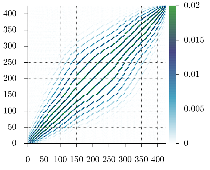
Figure 1.— Full pixel-pixel noise covariance matrix obtained from $N_{\textrm{nside}}=8$, $20^{\circ}$ smoothed maps over surviving pixels of pm10 mask for V band.

5.1.2 Mask

We see from Eqn 8, $\Delta\hat{\beta}_{s}(p)$ map may contain noisy pixels if corresponding pixels in the reconstructed synchrotron template, $\hat{T}_{4}(p)$, (or $\hat{T}_{3}(p)$), are also noise dominated. To avoid noisy reconstruction of spectral index map, we remove those pixels from all $10$ input frequency maps which contain weak synchrotron Stokes Q polarization signal. For this purpose, based upon the smoothed Stokes Q synchrotron template at K band, we make a mask which excise all pixels with absolute values less than 10$\mu K$ in antenna temperature unit. We call this mask pm10 mask and apply this mask to all frequency maps for reconstruction of spectral index map .

5.1.3 Physical Components

We use WMAP ‘base fit’ MCMC (Markhov Chain Monte Carlo) synchrotron and thermal dust polarization maps for our simulations. These maps are provided at $N_{\textrm{side}}=64$ at LAMBDA website. As mentioned at LAMBDA website, for some of the pixels of these maps, MCMC fitting resulted in errors. For both Q and U polarized synchrotron map at K band, using WMAP’s bit-coded error flag file, we first identify all pixels for which WMAP MCMC fit resulted in error. The process identifies a total of $1315$ pixels at $N_{\textrm{side}}=64$. Pixel value for each of these bad pixels is then replaced by the average pixel value of its nearest neighbors. If a bad pixel has one or more bad neighbours we average only over the good ones. Following similar procedure we obtain polarized thermal dust template at W band at $N_{\textrm{side}}=64$. We downgrade each of these two templates to $N_{\textrm{side}}=8$. We generate polarized CMB maps compatible to WMAP LCDM spectrum directly at $N_{\textrm{side}}=8$. We smooth both foreground templates and CMB maps by the Gaussian beam of FWHM = $20^{\circ}$.

5.1.4 Spectral Index Map

For spectral index we use WMAP ‘best-fit’ MCMC spectral index map. This map is provided by the WMAP science team at $N_{\textrm{side}}=64$. We downgrade this map at $N_{\textrm{side}}=8$ and subsequently smooth by a Gaussian beam of FWHM = $20^{\circ}$. This smoothed spectral index map defines our primary spectral index map, $\beta_{s}(p)$, for this work with which we compare the reconstructed spectral index map obtained by our method.

5.1.5 Detector Noise Maps and Covariance Matrix

Generating noise maps and thus modelling the noise properties in the low resolution maps are somewhat involved than simple smoothing operations that were needed to be performed on foreground templates and CMB maps at $N_{\textrm{side}}=8$ in Section 5.1.3. We take into account WMAP’s scan modulated detector noise pattern by using $N_{\textrm{obs}}(p)$ information associated with each nine-year Differencing Assembly (DA) map available at LAMBDA website at $N_{\textrm{side}}=512$. We first compute noise variance at each pixel following $\sigma^{2}(p)=\sigma^{2}_{0}/N_{\textrm{obs}}(p)$ at $N_{\textrm{side}}=512$ for all DA maps between K to V band. Since for each of Q and V bands two DA maps are available we simply average the variances of the corresponding DA’s at each pixel, to obtain noise variance map corresponding to average DA map within the frequency bands. For Planck LFI and HFI maps we use simple uniform white noise model. Pixel white noise levels, $\sigma(p)$, for Planck maps are obtained from Planck blue book specifications, $\sigma_{bb}$, which represents noise in the beam area of the corresponding map in unit of $\mu K/K$. Pixel noise levels for Planck maps at $N_{\textrm{side}}$ are then given by, $\sigma(p)=\sigma_{bb}T_{CMB}B_{fwhm}/\Delta\theta$, where $B_{fwhm}$ represents FWHM of Planck beams in arcmin, $\Delta\theta=6.9^{\prime}$, represents pixel size of $N_{\textrm{side}}=512$ map and $T_{CMB}=2.73K$.

In principle, one can use all the noise variance maps at $N_{\textrm{side}}=512$ corresponding to all frequency bands of Table 1 to obtain representations of noise maps at $N_{\textrm{nside}}=512$ and then downgrade them to $N_{\textrm{side}}=8$ for use in our simulation. However, one needs to simulate many such maps at $N_{\textrm{side}}=512$, since we need to obtain pixel pixel noise covariance at $N_{\textrm{side}}=8$ by downgrading the high resolution noise maps. Since generating noise maps at $N_{\textrm{side}}=512$ and subsequently downgrading them many times are computationally very expensive we device a completely equivalent approach which is computationally significantly fast compared to the former method. Instead of downgrading $N_{\textrm{side}}=512$ noise maps we obtain noise variance maps at $N_{\textrm{side}}=8$ by simply averaging over noise variance of all $N_{\textrm{side}}=512$ pixels lying inside each $N_{\textrm{side}}=8$ pixel. Such a method is always feasible for our method and does not introduce any pixel-pixel correlation at $N_{\textrm{side}}=8$ since noise in the original $N_{\textrm{side}}=512$ maps are uncorrelated from pixel to pixel. Using these noise variance maps we simulate noise maps at $N_{\textrm{side}}=8$. These noise maps are then smoothed by Gaussian beam of FWHM = $20^{\circ}$, to generate realistic noise maps at $N_{\textrm{side}}=8$ for each frequency band. We obtain $10000$ Monte-Carlo simulations of smoothed noise maps at $N_{\textrm{side}}=8$. Since the smoothing operations introduces pixel to pixel noise covariance we obtain full pixel to pixel noise covariance matrix over surviving pixels (after application of pm10 mask) at $N_{\textrm{side}}=8$ corresponding to each frequency band. We have shown noise covariance matrix for V band masked map, in Figure 1. Non-diagonal nature of this matrix indicates non-trivial noise properties in the maps.

Using the $N_{\textrm{side}}=8$ smoothed CMB Stokes Q polarized map, $Q_{c}(p)$, synchrotron and thermal dust templates ($Q_{0s}$ and $Q_{0d}$ respectively), spectral index map, $\beta_{s}(p)$ and detector noise map, $Q^{n}_{i}(p)$ ($i=1,2,...,n_{b}$) as obtained above we generate simulated frequency maps for WMAP and Planck frequency bands, using Eqn 2 and knowing the values of $a_{i}$. We use $\beta_{d}=2.0$, $\nu_{0s}=23$ GHz and $\nu_{0d}=94$ GHz in this work.

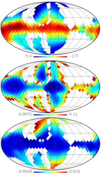
Figure 2.— Top panel: Mean synchrotron reconstructed spectral index map obtained from $1000$ simulations of this work. Middle panel: The standard deviation of spectral index map. Bottom Panel: Difference of top panel and input spectral index map.

5.2. Analysis

Since spectral indices of neither synchrotron, nor thermal dust components are known a priori, we perform reconstruction of all components defined by Eqn 5 for a suitable range of both of these indices. We vary $\beta_{0s}$ between $-2.65$ to $-3.05$ with a step of $-0.01$. For each of these values $\beta_{d}$ is varied between $1.80$ and $2.20$ with a step size $0.01$. For each pair ($\beta_{0s},\beta_{d}$), such generated, we compute shape vectors for all foreground template components. Combining these with the shape vector of CMB we estimate a set of weights using Eqn 15 to reconstruct all template components including CMB. For each pair ($\beta_{0s},\beta_{d}$), we form reconstructed frequency maps following Eqn 16 using all the reconstructed template components. We then form the difference map at each frequency by subtracting reconstructed frequency map from the corresponding input frequency map. The noise covariance of the $i^{th}$ difference map over the surviving pixels for a given pair of indices is given by the matrix, $N^{i,D}_{pp\prime}$, defined by Eqn 21. Once the difference map is formed we obtain $\chi^{2}(\beta_{0s},\beta_{d})$ for all indices following Eqn 22. Our best fit values for indices are the ones which minimizes $\chi^{2}$ over all indices. Using these values we obtain spectral index variation map following Eqn 8. We validate our method by performing $1000$ Monte Carlo simulations of entire procedure described above. We note that since CMB follows blackbody distribution its shape vector remain identical for all foreground indices and for all simulations. Since the weights as given by Eqn 15 depend only upon foreground and CMB shape vectors (without any dependence on random detector noise which vary from simulation to simulation) for reconstruction purpose of all components, we calculate these weights only once for the entire range of spectral indices and store them on the disk. We then use these weights to reconstruct all components for all Monte-Carlo simulations for all indices. Moreover, we also precompute Moore-Penrose generalized inverses of detector noise covariance matrices of all difference maps for all pairs of spectral indices $(\beta_{0s},\beta_{d})$ and store them on the disk. In effect a Singular Value Decomposition algorithm with cutoff $1.0\times 10^{-7}$ was used to implement Moore-Penrose inverses.

6. Results

6.1. Spectral Index Map

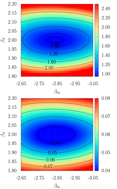
Figure 3.— Top panel: Variation of mean $\chi^{2}(\beta_{0s},\beta_{d})$ with respect to spectral indices obtained from $1000$ Monte Carlo simulations. Bottom panel: Standard deviation map of $\chi^{2}(\beta_{0s},\beta_{d})$ for any one of the $1000$ simulations.

For each simulation described in Section 5, we construct spectral index variation map, $\Delta\hat{\beta}_{s}(p)$, over the reference index, $\beta_{0s}$, following Eqn 8. The results for reconstruction of spectral index map are shown in Figure 2. The colored area of Mollweide projection of all the three panels shows the region on the sky that survives after applying pm10 mask. The top panel shows mean reconstructed synchrotron spectral index map, $\left<\hat{\beta}_{s}(p)\right>$, defined as, $\left<\hat{\beta}_{s}(p)\right>=\left<\beta_{0s,\textrm{min}}\right>+\left<\Delta\hat{\beta}_{s}(p)\right>$, where $\beta_{0s,\textrm{min}}$ denotes value of $\beta_{0s}$ (e.g., see Eqn 4) corresponding to $\chi^{2}_{min}$ and the average is performed over all $1000$ simulations. The middle panel is simple standard deviation map for any one of the reconstructed spectral index maps. The lower most panel shows the difference between average reconstructed index map and the input spectral index map, $\left<\hat{\beta}_{s}(p)\right>-\beta_{s}(p)$. Clearly, the difference map shows our method can accurately reconstruct spectral index map inside the pm10 mask. The reconstruction difference towards higher (lower) galactic coordinates becomes slightly larger due to weak polarized signal in these regions.

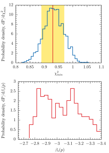
Figure 4.— Top panel: Probability density of minimum $\chi^{2}$ values obtained from $1000$ simulations. Red vertical line shows the location of sample mean corresponding to $\chi^{2}_{min}=0.93$. Light golden band around the mean value shows regions within 1$\sigma$ deviation. Bottom panel: Probability density function of pixel indices obtained from smoothed input spectral index map after application of pm10 mask.

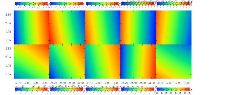
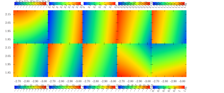
Figure 5.— Top panel: Weights for reconstruction of $Q_{0s}(p)$. Bottom panel: Weights for reconstruction of $Q_{0s}(p)\Delta\beta_{s}(p)$. For any given panel, plots in consecutive rows from left to right indicate respectively weights for K, A, Ka, Q, B, C, V, D, E and F frequency bands.

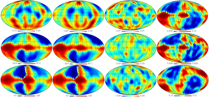
Figure 6.— Results for ML template reconstruction for CMB (top panel), thermal dust (middle panel) and synchrotron (bottom panel). Units for all colormaps are in $\mu K$ temperature unit (thermodynamic for CMB, antenna for foreground components).

For any given Monte-Carlo simulation $\chi^{2}(\beta_{0s},\beta_{d})$ values shows a clear minimum, $\chi^{2}_{min}$, at some values of $(\beta_{0s},\beta_{d})=(\beta_{0s,\textrm{min}},\beta_{d,\textrm{min}})$. Although a topographical plot of $\chi^{2}(\beta_{0s},\beta_{d})$ depends upon the particular random simulation under consideration, the features of such plots that arise on the average due to foregrounds, CMB and detector noise, can be studied by making a plot of $\left<\chi^{2}(\beta_{0s},\beta_{d})\right>$ (where the average is performed over all $1000$ simulations for each pair $(\beta_{0s},\beta_{d})$) with respect to both indices. We have shown this at the top panel of Figure 3. The elongated contours of this plot shows the relatively higher sensitivity of the data with the variation of synchrotron spectral index compared to the same variation of dust spectral index. In the bottom panel of this figure we show standard deviation map of $\chi^{2}$ values for all indices. Lower standard deviation values around $\left<\chi^{2}_{min}\right>$ indicates minimum is recovered satisfactorily by our method. Using results from Monte Carlo simulations we estimate average value of $(\beta_{0s,\textrm{min}},\beta_{d,\textrm{min}})$ corresponding to $\chi^{2}_{min}$ as $(-2.84\pm 0.01,2.00\pm 0.004)$. Small error on the spectral index values corresponding to $\chi^{2}_{min}$ shows that our method can reliably recover global spectral indices.

Using the Monte Carlo simulations we find that values of $\chi^{2}_{min}$ is distributed over a narrow range of $0.82$ to $1.05$. A plot of histogram of $\chi^{2}_{min}$ is shown in top panel of Figure 4. We estimate, $\left<\chi^{2}_{min}\right>=0.93$, averaging over $1000$ Monte-Carlo simulations, with sample standard deviation $0.04$. The probability density function of this figure, follows a very symmetric distribution for $\chi^{2}_{min}$. This can be expected due to very large number of degrees of freedom ($\sim 4260$) available in the analysis. In the bottom panel of this figure we have shown probability distribution of $20^{\circ}$ smoothed $N_{\textrm{side}}=8$ input spectral index map, from the region that survives after application of $\it pm10$ mask. A bimodal structure of the distribution is readily identifiable corresponding to spectral indices $\sim-2.85$ and $-3.16$ respectively. Comparing these values with the mean reconstructed spectral index $-2.84\pm 0.01$, it is interesting to note that our method picks out the peak corresponding to a flatter index, from available, a pair of doubly degenerate ones.

6.2. Weight

One very important component of this work are the weights. We show weights for reconstruction of $Q_{0s}(p)$ and $Q_{0s}(p)\Delta\beta_{s}(p)$ templates for the entire range of spectral indices, respectively in the top and bottom panel of Figure 5. At the low frequency side, where synchrotron emission is dominant weights tend to be positive for all indices. We see this for K, A and Ka bands. For all other bands except F band, weights are negative for all indices. For F band weights become positive for all indices to cancel out signals from CMB, thermal dust, $Q_{0s}(p)\Delta\beta_{s}(p)$ and at the same time to preserve $Q_{0s}$. For reconstruction of $Q_{0s}(p)\Delta\beta_{s}(p)$ template weights must completely project out its shape vector from the data, at the same time, the weight vector need to be orthogonal to shape vectors of synchrotron and other components. Because of close analytical similarity in the shape vectors of $Q_{0s}(p)$ and $Q_{0s}(p)\Delta\beta_{s}(p)$ the orthogonality condition leads to somewhat larger magnitude of weights for $Q_{0s}(p)\Delta\beta_{s}(p)$ than $Q_{0s}(p)$ template. Relatively larger magnitude of weights can easily be seen from the second panel than the first one. For the second panel and for K band, weights take largest negative value, since, from the expression of shape vector for $Q_{0s}(p)\Delta\beta_{s}(p)$ component, ($a(\nu)(\nu/\nu_{0s})^{-\beta_{0s}}\ln(\nu/\nu_{0s})$), shape vector has a zero component at K band. For low frequency A, Ka, Q, B bands all weights are positive indicating its larger shape vector at lower frequency. For V, C, D and E bands weights become negative, since shape vector decreases in this frequency range. Finally for F band weights again become positive to project out $Q_{0s}(p)\Delta\beta_{s}(p)$ component completely and to cancel out rest of the components.

6.3. CMB and Foreground

As associated results of our method, we reconstruct ML templates for all components using the best fit spectral index values $\beta_{0s,\textrm{min}},\beta_{d,\textrm{min}}$ corresponding to $\chi^{2}_{min}$ obtained in Section 6.1. We show the results in Figure 6. Unlike the case for reconstructed synchrotron spectral map, we do not apply any mask on the recovered templates, since CMB and foreground signals are expected to be stronger than the spectral index variations. Top, middle and bottom panels of this figure show results for CMB, thermal dust and synchrotron template reconstruction respectively, obtained from a randomly chosen Monte Carlo simulation with seed = $100$. All the color maps of this figure are in $\mu K$ unit (thermodynamic for CMB, antenna for foreground templates). Following usual row, column convention of a matrix, we represent any image of this figure by the pair $(i,j)$. $(1,1)$ image represents reconstructed CMB map against the input CMB map for the same simulation, shown as $(1,2)$ image. As one can easily visually identify the large scale features of these two maps are very nearly identical. $(1,3)$ image shows the difference between reconstructed and input CMB map and hence is dominated by residual detector noise. The noisy nature of the difference map is also indicated by the symmetric color table plotted below $(1,3)$ image. The $(1,4)$ image represents the standard deviation map estimated from set of all $(1,3)$ maps resulting from $1000$ Monte Carlo simulations of component separation algorithm. As expected, the standard deviation map clearly indicates a scan modulated noise pattern as applicable for WMAP observations. There exist some foreground induced errors on the galactic plane. Such errors can be reduced by extending our method to a second order perturbative analysis.

The $(2,1)$ image represents reconstructed thermal dust template at $217$ GHz for seed = $100$. The reconstructed template matches very well with the input thermal dust template at the same frequency, viz., $(2,2)$ image. The difference between reconstructed and input template ($(2,3)$ image) is dominated by noise. The standard deviation map for reconstructed thermal dust template is shown as $(2,4)$ image. Clearly, WMAP’s scan modulated noise pattern is visible in this figure. There also exist some residual foregrounds error in this map, which again can be eliminated by performing a higher order perturbative analysis.

The $(3,1)$ image shows reconstructed synchrotron template at $23$ GHz for the same random seed. The input synchrotron template at $23$ GHz is shown as $(3,2)$ image. Both these maps match with each each other very well. The difference of the first and second maps is shown as (3,3) image. The standard deviation map, image $(3,4)$, shows the scan modulated detector noise pattern, without any visible signature of residual foreground error.

7. Discussion & Conclusion

Reconstruction of CMB and foreground components jointly from microwave observations is a primary task for cosmologists. This can be achieved relatively easily if i) observed sky signal consists of only those components that have rigid frequency scaling all over the sky ii) detector noise is negligible and iii) total number of these components is less than or equal to total number of observed frequency bands. However, the task is complicated when spectral index of any one of the components varies with sky positions. The stronger the variation effectively one gets more components with rigid frequency scaling, which, if not taken into account in the analysis, may cause the results to be biased, or at the least difficult to interpret. The scenario becomes even worse in the presence of non-negligible detector noise. We have shown that in the presence of foregrounds following power law model with spatially varying index and small amount of detector noise one can recover the spectral index variation map reliably from the WMAP and Planck Stokes Q observations without any need to model foregrounds and or CMB in terms of any model templates. The only assumption we have made in this work is a power law model for the foregrounds. However, this is not a necessary condition for our method to work, since one can directly fit for the shape vectors for all components by expanding the parameter space. Then with the help of perturbative expansion of the spectral index variation one can reconstruct the index variation map. Since the spectral index variation for synchrotron component is small compared to other emissions (specifically, compared to synchrotron emission amplitude itself), and can be masked by the presence of comparable level of detector noise contamination. we chose to work with maps containing low level of detector noise, by smoothing the frequency maps by a $20^{\circ}$ beam window function. We use full pixel-pixel detector noise covariance matrix to accurately model the smoothed detector noise pattern, and thus for better reconstruction of spectral index map. The condition for large beam window can be relaxed easily for experiments, or for sky regions with negligible detector noise. A very interesting future project will be to apply the method on the Planck polarized observations combined with WMAP, and with polarization sensitive, low noise, future CMB observations like CMBPol. For very low noise experiments in future, it would be very useful to extend our method up-to second order perturbative analysis for even more accurate understanding of cosmological and astrophysical information contained in data.

We summarize main results and conclusions of this work as follows:

1. We present and implement a first order perturbative method to estimate variation of synchrotron spectral index over the microwave sky using simulated Stokes Q observations of WMAP K, Ka, Q, V, Planck LFI, and three lowest frequency Planck HFI frequency bands. We validate the method by performing $1000$ Monte Carlo simulations over regions of the sky dominated by synchrotron Stokes Q signal. Our results suggest that, following the first order analysis synchrotron spectral index variation map can be reconstructed reliably by our method with a narrow error margin.

2. As accompanying results of this work, we reconstruct CMB, thermal dust and synchrotron template components. An error estimation on the reconstructed templates suggest that the template components can be reconstructed reliably by our method.

3. Our reconstructed templates and best fit spectral indices are ML estimates.

4. The perturbative method of this work possesses an interesting property that it can be tuned to the data with an accuracy, as allowed by the data. This could be particularly very useful for CMB and foreground component separation problem if the data is insufficient to constrain an otherwise completely accurate model, due to underlying degeneracies in the foreground components.

The work presented in this paper will allow an improved estimation of cosmological signal due to its detailed foreground modelling in terms of variation of spectral indices. It will be useful to extract astrophysical information about galactic synchrotron emission, in particular, information about the galactic cosmic ray electrons and the magnetic field. Finally, the method can be used to extract jointly all foregrounds components along with CMB signal from CMB observations.

RS acknowledges research grant SR/FTP/PS-058/2012 by SERB, DST. Some of the results of this paper were obtained using publicly available HEALPix (Górski et al. (2005)) package available from web page http://healpix.sourceforge.net. We acknowledge the use of the Legacy Archive for Microwave Background Data Analysis (LAMBDA), part of the High Energy Astrophysics Science Archive Center (HEASARC). HEASARC/LAMBDA is a service of the Astrophysics Science Division at the NASA Goddard Space Flight Center.

References

- Baksalary et al. (2003) Baksalary, J. K., Baksalary, O. M., & Trenkler, G. 2003, Linear Algebra and its Applications., 372, 207
- Bennett et al. (2003) Bennett, C. L., Hill, R. S., Hinshaw, G., et al. 2003, Astrophys. J. Suppl. Series, 148, 97
- Bennett et al. (2013) Bennett, C. L., Larson, D., Weiland, J. L., et al. 2013, ApJS, 208, 20
- Bennett (2012) Bennett, C. L., e. 2012, ApJS, arXiv:1212.5225
- Bouchet & Gispert (1999) Bouchet, F. R., & Gispert, R. 1999, New A, 4, 443
- Bouchet et al. (1999) Bouchet, F. R., Prunet, S., & Sethi, S. K. 1999, MNRAS, 302, 663
- Bunn et al. (1994) Bunn, E. F., Fisher, K. B., Hoffman, Y., et al. 1994, ApJ, 432, L75
- consortium (2005) consortium, T. P. 2005, PLANCK - The Scientific Programme, ESA-SCI(2005)1, PLANCK Bluebook (ESA-SCI(2005)1)
- Davies et al. (1996) Davies, R. D., Watson, R. A., & Gutierrez, C. M. 1996, MNRAS, 278, 925
- Delabrouille et al. (2009) Delabrouille, J., Cardoso, J.-F., Le Jeune, M., et al. 2009, A&A, 493, 835
- Dobler (2012) Dobler, G. 2012, ApJ, 760, L8
- Eriksen et al. (2008a) Eriksen, H. K., Dickinson, C., Jewell, J. B., et al. 2008a, ApJ, 672, L87
- Eriksen et al. (2008b) Eriksen, H. K., Jewell, J. B., Dickinson, C., et al. 2008b, ApJ, 676, 10
- Fuskeland et al. (2014) Fuskeland, U., Wehus, I. K., Eriksen, H. K., & Næss, S. K. 2014, ApJ, 790, 104
- Gold et al. (2009) Gold, B., Bennett, C. L., Hill, R. S., et al. 2009, ApJS, 180, 265
- Gold et al. (2011) Gold, B., Odegard, N., Weiland, J. L., et al. 2011, ApJS, 192, 15
- Górski et al. (2005) Górski, K. M., Hivon, E., Banday, A. J., et al. 2005, ApJ, 622, 759
- Hinshaw et al. (2007) Hinshaw, G., Nolta, M. R., Bennett, C. L., et al. 2007, Astrophys. J. Suppl. Ser., 170, 288
- Hinshaw et al. (2013) Hinshaw, G., Larson, D., Komatsu, E., et al. 2013, ApJS, 208, 19
- Hobson et al. (1998) Hobson, M. P., Jones, A. W., Lasenby, A. N., & Bouchet, F. R. 1998, MNRAS, 300, 1
- Maino et al. (2002) Maino, D., Farusi, A., Baccigalupi, C., et al. 2002, MNRAS, 334, 53
- Meyer (1973) Meyer, C. D. J. 1973, SIAM Jurnal on Applied Mathematics, 24, 315
- Moore (1920) Moore, E. H. 1920, Bull. Am. Math. Soc., 26, 394, unpublished address. Available at http://www.ams.org/journals/bull/1920-26-09/S0002-9904-1920-03322-7/S0002-9904-1920-03322-7.pdf.
- Penrose (1955) Penrose, R. 1955, Mathematical Proceedings of the Cambridge Philosophical Society, 51, 406
- Planck Collaboration et al. (2013) Planck Collaboration, Ade, P. A. R., Aghanim, N., et al. 2013, A&A, 554, A139
- Planck Collaboration et al. (2014) —. 2014, A&A, 571, A23
- Planck Collaboration et al. (2015a) Planck Collaboration, Adam, R., Ade, P. A. R., et al. 2015a, ArXiv e-prints, arXiv:1502.05956
- Planck Collaboration et al. (2015b) —. 2015b, ArXiv e-prints, arXiv:1502.01588
- Planck Collaboration et al. (2015c) Planck Collaboration, Ade, P. A. R., Aghanim, N., et al. 2015c, ArXiv e-prints, arXiv:1502.01589
- Planck Collaboration et al. (2015d) —. 2015d, ArXiv e-prints, arXiv:1502.01594
- Planck Collaboration et al. (2015e) —. 2015e, ArXiv e-prints, arXiv:1502.01592
- Planck Collaboration et al. (2015f) —. 2015f, ArXiv e-prints, arXiv:1502.01593
- Planck Collaboration et al. (2015g) —. 2015g, ArXiv e-prints, arXiv:1502.02114
- Planck Collaboration et al. (2015h) —. 2015h, ArXiv e-prints, arXiv:1506.06660
- Platania et al. (1998) Platania, P., Bensadoun, M., Bersanelli, M., et al. 1998, Astrophys. J., 505, 473
- Reich & Reich (1988) Reich, P., & Reich, W. 1988, A&AS, 74, 7
- Remazeilles et al. (2011) Remazeilles, M., Delabrouille, J., & Cardoso, J.-F. 2011, ArXiv e-prints, arXiv:1103.1166
- Saha (2011) Saha, R. 2011, ApJ, 739, L56
- Saha et al. (2008) Saha, R., Prunet, S., Jain, P., & Souradeep, T. 2008, Phys. Rev. D, 78, 023003
- Tegmark (1998) Tegmark, M. 1998, ApJ, 502, 1
- Tegmark et al. (2003) Tegmark, M., de Oliveira-Costa, A., & Hamilton, A. J. 2003, Phys. Rev. D, 68, 123523
- Tegmark & Efstathiou (1996) Tegmark, M., & Efstathiou, G. 1996, Mon. Not. R. Astron. Soc., 281, 1297
- Tegmark et al. (2000) Tegmark, M., Eisenstein, D. J., Hu, W., & de Oliveira-Costa, A. 2000, ApJ, 530, 133