A Hedged Monte Carlo Approach to Real Option Pricing

Abstract

In this work we are concerned with valuing optionalities associated to invest or to delay investment in a project when the available information provided to the manager comes from simulated data of cash flows under historical (or subjective) measure in a possibly incomplete market. Our approach is suitable also to incorporating subjective views from management or market experts and to stochastic investment costs.
It is based on the Hedged Monte Carlo strategy proposed by Potters et al (2001) where options are priced simultaneously with the determination of the corresponding hedging. The approach is particularly well-suited to the evaluation of commodity related projects whereby the availability of pricing formulae is very rare, the scenario simulations are usually available only in the historical measure, and the cash flows can be highly nonlinear functions of the prices.

1 Introduction

The use of quantitative finance techniques to evaluate projects while trying to capture the value of active management and flexibility is known by the name of Real Option Analysis (ROA). The importance of capturing such “non-passive” value of projects can be a decisive factor when trying to decide upon investment within a portfolio of projects. Most of the classical applications of ROA involves vanilla American options as the case of the option to postpone a project, or to abandon it. However, when considering projects related to capacity planning, chemical or petrochemical plants, oil refining, or indeed any commodities-based project, a significant increase in complexity arises. Under these conditions, recurring problems that are encountered in real options, as dealing with market incompleteness, become particularly acute.

In many cases, the company has access to financial instruments that strongly correlate with the projects, and sometimes, as in the case of commodities companies, even with their final product. Thus, the company can hedge some of its exposition yielded by a project, but usually not all of it, by an appropriate hedging portfolio. This suggests that a hedging approach based on Monte Carlo simulations can be a plausible alternative for pricing such real options. Indeed, on one hand quadratic hedging has been used to price financial options in incomplete markets, and it is based on the local minimization of a proxy to variance, that is readily recognized as a risk measure by managers. On the other hand, Monte Carlo approach has been often used when dealing both with options involving many assets—as baskets, rainbow, etc.—or when asset price models are not readily available.

The aim of this work is to propose the use of the so-called Hedged Monte Carlo Method—Monte Carlo pricing through quadratic hedging—to price such complex options.

The plan for this article goes as follows: We close this introductory section with a description of the project evaluation problem we are considering, a short methodological review of the different approaches to real options, and its analysis by means of hedging with financial instruments. In Section 2 we present an approach to evaluating real options based on the Hedged Monte Carlo (HMC) method of Potters et al (2001).

It has a number of desirable features: it uses the dynamics under the historical/subjective measure; it allows for an easy determination of the optimal exercise boundary, it has low variance, and allows for an assessment of the nonhedgeable risk. Furthermore, the oracle approach easily allows to incorporate managerial views in many different levels: it can either accommodate views of different managers of related projects, or more global corporative views and scenarios. The method developed is explored in Section 3 with some examples and a few case studies. We conclude in Section 4 with some final comments and suggestions for further developments.

1.1 Real options analysis

The use of mathematical finance techniques has been continuously growing in recent times as a tool to capture the value of flexibility in projects. A classical account can be found in the books of Dixit and Pindyck (1994) and Trigeorgis (1999). The subject blossomed under different names but is generally known Real Options. See also Myers (1977); Tourinho (1979); Titman (1985); Brennan and Schwartz (1985); McDonald and Siegel (1986); Trigeorgis and Mason (1987); Paddock et al (1988); Dixit (1989); Pindyck (1991); Ingersoll and Ross (1992).

The original framework identifies the Net Present Value of the project as a stochastic process correlated with a tradable risky asset. The risky asset is termed the twin or spanning asset whereas the project value is sometimes referred as the surrogate asset. Subsequent approaches take this identification very far. Indeed, one cannot expect to have a traded asset with a perfect correlation with the project, since this would mean that project risk is totally diversifiable, and hence replicable via financial markets. An alternative view, is to look for an asset, typically an index, that yields a high correlation with the project returns. This is known as the modern approach. Other approaches exist. See Borison (2005) for a classification, the discussion in Jaimungal and Lawryshyn (2011), and the remarks in Section 1.4.

A very strong critique of the real option approach was presented by Hubalek and Schachermayer (2001). There they show, by means of a simple example, that the use of no-arbitrage techniques to nontradable surrogate assets can lead to arbitrary (very high or very low) no-arbitrage option prices. This in turn shows that the economic use of real options in the context of incomplete markets is highly questionable. In the same work, they also show that a variance minimization of the hedging error could be a way out of the economical impasse caused by the lack of completeness of the market.

1.2 Complex structured real options

We are concerned with the practical problem of quantitatively evaluating projects under uncertainty from different scenarios taking into account flexibility of the projects and the possibility of partial hedging with financial instruments. We assume that we have available a fairly large number of scenarios organized in a time series and that connected to the different scenarios we have an oracle that produces the cash flows associated to each scenario. The scenarios in turn are linked to traded assets or financial instruments which may be used for hedging the project. Figure 1 describes the situation.

Figure 1: Description of the oracle producing the cash flows at time $t$ and scenario $i$.

This framework can arise when planning chemical plants or oil refineries. See for example Moro et al (1998), Papageorgiou (2009), Sahinidis et al (1989), Shapiro (2009), Oldenburg et al (2007). It also naturally appears when using real option techniques for capacity planning. See Mittal (2004), Novaes and Souza (2005), Chen et al (2007). In most of these problems, the markets are overall incomplete, unless under very simplifying assumptions. In addition, such incompleteness will also imply that data will be only available under the historical measure.

We shall now consider different ingredients in such complex options. The first one, stems from the fact that many corporations predict in a fairly precise way their cash flows using a black box (oracle) whose stochasticity only comes through the inputs from the different assets, supply/demand curves, and production curves. Yet, such oracle depends on the prices of many (stochastic) assets as well as on non-tradable quantities. This is depicted in the Figure 1.

More generally, the cash flows may be produced by simplified models that incorporate algorithms or analytical procedures.

Among the challenges that are present in the evaluation of projects under uncertainty, especially those linked to commodity enterprises, we single out the following:

• Historical measure: The simulations are usually presented in the historical measure. Furthermore, the scenarios are provided by management and are loaded with views from advisors or sector specialists. In fact, some corporations delegate the scenario generation to part of the board of directors or an independent division.

• Managerial views: It is crucial to incorporate managerial views in the cash flows, as well as automated decisions. An example would be a commodity trading company that has a limited amount of storage capacity for different products. According to the relative prices and profits it may automatically determine how much of each product it would store.

• Market incompleteness: The hedging is performed in incomplete financial markets. In fact, sometimes the firm does not have access to the liquidity provided by the financial markets. In other cases, regulations might preclude the management to hold some speculative positions to fully hedge against market variations.

• Unhedgeable risks: Investment decisions on commodity related projects have to take into account not only the hedgeable risks, but also the unhedgeable ones. For instance, the decision of exploring an oil field is highly dependent on its production curve and also on ecological risks associated to the operation.

• Multiple assets: Investment decisions may depend on the relative value of several traded underlyings. Such assets might have general correlation structures ranging from low to high cross-correlation. Thus, the hedging might have to be very diversified.

1.3 Real option analysis through hedging

The approach suggested here to attack the general problem mentioned above can be loosely described as a risk minimization one where the project valuation is performed by constructing a portfolio that includes the project delay optionality and the possible hedging of such project by tradable assets. By a methodology introduced by Potters et al (2001) (see also Grasselli and Hurd (2004)) one can compute different financial options (including American and Bermudian ones) by a recursive risk minimization of historical-measure simulated paths. The importance of using historical simulations in the solution of this problem is that managers consider their decisions by looking at observed prices of different commodities and assets. We shall refer to the methodology developed in Potters et al (2001) by the Hedged Monte Carlo method (HMC).

Another motivation for the methodology presented here is the critique to the traditional no-arbitrage arguments of real option theory present in the work of Hubalek and Schachermayer (2001). In the latter, the idea of minimizing the variance is considered as an alternative to the shortcomings caused by market incompleteness. A number of different approaches have been developed to deal with incomplete markets. To cite a few: indifference pricing, minimal martingale measure, and minimal entropy measure.

The idea of using HMC or Monte Carlo algorithms to compute option prices in incomplete markets is not new. See, for example, the work of Primbs and Yamada (2008) and the references therein. It can also be traced to the preprint of Grasselli and Hurd (2004). The novelty of the approach suggested herein is the idea of incorporating the different cash flows in the evaluation, producing the different statistics that may be helpful for the manager and allow for the possibility of incorporating managerial views in the simulations. As it turns out, the HMC methodology corresponds to choosing the minimal martingale measure of Schweizer and Föllmer (1988). See Lipp (2012) and Gastel (2013) and references therein for details on such connection.

1.4 Remarks on alternative approaches

We shall now briefly review the various methodologies available to price real options.

Hedging Public and Private Risks: As observed in the works of Borison (2005) and of Jaimungal and Lawryshyn (2011), one of the main issues in evaluating different types of projects is whether the source of risk is public or private. For projects with returns that are highly correlated to the market, risk mitigation should be almost completely achievable by hedging it with traded assets. In most approaches, the project is assumed to be perfectly correlated to a single asset, and hence replicable. Notice that for projects which have a diverse range of products, it might be necessary to use a basket of hedging assets.

On the other hand, projects with mainly private risks, such as for instance R&D, are unlikely to be hedged with the use of traded assets. Moreover, in some cases the valuation of the project can be highly dependent on management estimates. Thus, one can think of such estimates as a non-traded asset that contributes to the value of the project.

From the point of view of utility theory, this can be more precisely measured by specifying the firm’s preferences through a utility function, and thus one can think of using indifference pricing. This approach was pursued in a number of works, in particularly in the work of Henderson and Hobson (2002), of Grasselli and Hurd (2004), and of Grasselli and Hurd (2007).

The Classical Method: As mentioned in the introduction, the classical methodology of pricing real options assumes that there is a spanning asset that is highly correlated to the net present value (NPV) of the project. One example of such methodology is the so-called Marketed Asset Disclaimer (MAD) Approach is based on the idea of taking the NPV distribution both as the value of the project and as the underlying (tradable) asset. Then, model the asset with a stochastic dynamics and perform Risk-Neutral pricing, perhaps accounting for non-traded issues. See for example Copeland and Antikarov (2001) and Copeland and Tufano (2004). Among the advantages we mention that it mimics the standard mathematical finance approach, the theory is fairly simple and many out-of-the-box numerical methods are available. As for the disadvantages, besides the general criticism mentioned before in reference to the work of Hubalek and Schachermayer (2001), we should also note that often very few data is available for calibration. This makes the choice of the underlying dynamics somewhat arbitrary. Furthermore, for each project, a calibration/choice of underlying dynamics is necessary. This ambiguity is typically tackled by a simplifying assumption on the dynamics, which will hopefully be consistent with the market scenarios.

Monte Carlo Based Approaches: In many situations the project or the firm has a simulator that we shall refer from now on as an oracle. Such oracle produces information about the cash flows associated to different projects or optionalities for different scenarios which in turn are generated from inputs of tradable assets. The idea is then to take the oracle output as the payoff distribution, and use the method of Longstaff and Schwartz (2001) to compute the corresponding conditional expected values subject to the traded asset prices. This requires the underlying(s) to be simulated in the risk-neutral measure or taking into account the market price of risk in the final result.

Among the pros of such approach, we should mention that it uses fully the oracle information towards the option evaluation, it is easily integrated and automated with the oracle thus leading to a project independent pricing mechanism. Furthermore, it has a good managerial appeal. As for the cons, we have that since the simulation is performed on the oracle data, the realizations are restricted to the ones generated by the oracle. This can impair the quality of the results obtained. Furthermore, the risk-neutral calibration of the scenario generation that will provide inputs to the oracle might be very cumbersome and requires extra work.

Datar-Mathews (DM) Method: In the method proposed by Mathews et al (2007) one assumes that it is given the NPV distributions (usually by management). Then, one performs a Monte Carlo simulation to replicate the distribution at the given times and to produce a simulated process for the underlying asset.

Among the advantages, we can mention that it is easily implemented and has great managerial appeal. Yet, there is lack of theory to justify such approach.

Jaimungal-Lawryshyn (JL): The work of Jaimungal and Lawryshyn (2011) includes an extension of DM method as follows: They take the NPV distributions and choose an observable sector index (not-traded on their paper) that is highly correlated with cash flows. They choose a dynamics for this index and based on the dynamics, find the payoff functions that yield the NPV distribution as a function of this market index. Then, they identify the value of the project as expected values of these payoffs (very much line in DM’s method). Finally, they choose a correlated (if possible) traded asset or index and perform a risk-neutral valuation using a Minimal Martingale Measure.

Among the advantages of this method, we can cite that as in the DM method, it integrates the managerial view with the Real Option Analysis. Thus it has a good managerial appeal. Furthermore, the theory is more sound. Yet, the market index might not be easily available and one still needs to calibrate the model to the index. This step might be hard if the data is not abundant.

2 The Hedged Monte Carlo Approach and Minimal Martingale Measures

Since the typical data that will be used for the method comes from simulations, it will be naturally discrete in time. Thus, it is natural to adopt a discrete time approach for the algorithm. In this vein, we begin by reviewing the theory for quadratic hedging in discrete time and how it can be used to price contingent claims. This will follow closely the exposition of Föllmer and Schied (2004). Then, we proceed on to discussing the algorithm itself, and present a brief remark about its relation to a continuous version of the problem.

2.1 Hedging in discrete time within an incomplete market: a review

In an incomplete market setting, from its very definition, a self-financing replicating strategy is not usually available. In this scenario, one might give up the replicating property, and look for self-financing hedging strategies that control the down side risk—evaluated by means of a risk measure. See for example the work of Föllmer and Schied (2004). Alternatively, one enforces a replicating strategy and looks for the cheapest strategy with this property. In this latter case, a very popular strategy among practitioners is the minimization of the quadratic tracking error Schweizer (2008). This choice leads to strategies that are self-financing in the mean under very mild assumptions, that we now briefly review.

As usual, we assume to be in a filtered probability space $(\Omega,\mathcal{F}_{T},{\mathbb{P}})$ and write $L^{2}({\mathbb{P}})=L^{2}(\Omega,\mathcal{F}_{T},{\mathbb{P}})$, where ${\mathbb{P}}$ denotes the historical measure. In what follows, $\xi^{N}$ denotes the investment (short or long) in the numéraire asset, and $\xi$ denotes the position on $d$ risk assets, with prices given by a $d$-dimensional stochastic process $X$. Furthermore, $X$ and $V$ denote discounted prices with respect to a risk-free process.

Definition 2.1

A trading strategy is a pair of stochastic processes $(\xi^{N},\xi)$, where $\xi^{N}_{t}$ is an adapted process and $\xi$ is a $d$-dimensional predictable process. The discounted value of the portfolio is

$$V_{t}:=\xi^{N}_{t}+\xi_{t}\cdot X_{t}$$

The gain process is

$$G_{t}:=\sum_{s=1}^{t}\xi_{s}\cdot\left(X_{s}-X_{s-1}\right).$$

The cost process is defined as

$$C_{t}:=V_{t}-G_{t}.$$

Let $H$ denote a random claim, and assume that

1. $H\in L^{2}({\mathbb{P}})$;

2. $X_{t}\in L^{2}(\Omega,\mathcal{F}_{T},{\mathbb{P}};\mathbb{R}^{d})$, for all $t$.

Definition 2.2

An admissible $L^{2}$-strategy for $H$ is a trading strategy such that it is replicating, i.e.,

$$V_{T}=H\quad{\mathbb{P}}\,\text{ a.s.},\quad$$

and such that both the value process and the gain process are square-integrable, i.e.,

$$V_{t},G_{t}\in L^{2}({\mathbb{P}}),\,\forall t\in[0,T].$$

We can now introduce a suitable risk process

Definition 2.3

Let $(\xi^{N},\xi)$ be an $L^{2}$-admissible strategy. The corresponding local risk process is given by

$$R^{\mathrm{loc}}_{t}(\xi^{N},\xi)={\mathbb{E}}[(C_{t+1}-C_{t})^{2}|\mathcal{F}_{t}].$$

Let $(\hat{\xi}^{N},\hat{\xi})$ be an $L^{2}$-admissible strategy with value process $\hat{V}_{t}$. This strategy is said to be a locally risk-minimizing strategy if, for each $t$, we have that

$$R^{\mathrm{loc}}_{t}(\hat{\xi}^{N},\hat{\xi})\leq R^{\mathrm{loc}}_{t}(\xi^{N},\xi),\quad{\mathbb{P}}\,\text{a.s.}$$

for each $L^{2}$-admissible strategy whose value process $V_{t}$ satisfies $V_{t+1}=\hat{V}_{t+1}$.

Definition 2.4

A trading strategy is a mean self-financing strategy, if its corresponding cost process is a martingale, i.e.:

$${\mathbb{E}}[C_{t+1}-C_{t}|\mathcal{F}_{t}]=0.$$

Definition 2.5

We say that two adapted processes $U$ and $V$ are strongly orthogonal if

$$\mathop{\mathrm{cov}}(U_{t+1}-U_{t},V_{t+1}-V_{t}|\mathcal{F}_{t})=0,$$

where $\mathop{\mathrm{cov}}$ denotes the conditional covariance, i.e., $\mathop{\mathrm{cov}}(A,B|\mathcal{F}_{t})={\mathbb{E}}[AB|\mathcal{F}_{t}]-{\mathbb{E}}[A|\mathcal{F}_{t}]{\mathbb{E}}[B|\mathcal{F}_{t}]$.

The following result (see Föllmer and Schied (2004)) guarantees the existence of the corresponding hedge:

Theorem 2.1

1. An $L^{2}$-admissible strategy is locally risk minimizing if, and only if, it is mean self-financing, and its cost process is strongly orthogonal do $X$.

2. There exists a locally risk minimizing strategy if, and only if, $H$ admits the so-called Follmer-Schweiser decomposition:

   $$H=c+\sum_{t=1}^{T}\xi_{t}\cdot(X_{t}-X_{t-1})+L_{T},\quad{\mathbb{P}}\,\text{-a.s.},$$

   where $c$ is a constant, $\xi$ is a $d$-dimensional predictable process, such that $\xi_{t}\cdot(X_{t}-X_{t-1})\in L^{2}({\mathbb{P}})$ for each $t$, and $L$ is a square-integrable martingale that is strongly orthogonal to $X$, and satisfies $L_{0}=0$.

   In this case, the locally risk-minimizing strategy $(\hat{\xi}^{N},\hat{\xi})$ is given by :

   $$\hat{\xi} =\xi$$

   $$\hat{\xi}^{N}_{t} =c+\sum_{s=1}^{t}\xi_{s}\cdot(X_{s}-X_{s-1})+L_{t}-\xi_{t}\cdot X_{t}.$$

   Notice that the associated cost process is $C_{t}=c+L_{t}$.

2.2 Pricing by risk minimization

The proof of Theorem 2.1 is actually constructive and yields the following algorithm:

Algorithm 2.1

1. Set $\hat{V}_{T}:=H$;

2. For $t=T-1$ down to $t=0$ do

   1. Set

      $$(\hat{V}_{t},\hat{\xi}_{t+1}):=\mathop{\mathrm{argmin}}_{(V_{t},\xi_{t+1})}{\mathbb{E}}\left[\left(\widehat{V}_{t+1}-(V_{t}+\xi_{t+1}\cdot(X_{t+1}-X_{t}))\right)^{2}\big{|}\mathcal{F}_{t}\right];$$ (2.1)

3. Set $\hat{C}_{t}:=\hat{V}_{t}-\sum_{s=1}^{t}\hat{\xi}_{s}\cdot(X_{s}-X_{s-1})$, $t=0,\cdots,T$;

4. Set $\hat{c}:=\hat{C}_{0}$;

5. Set $\hat{L}_{t}:=\hat{C}_{t}-\hat{c}$, $t=0,\cdots,T$;

6. Set ${\hat{\xi}^{N}}_{t}:=\hat{c}+\sum_{s=1}^{t}\hat{\xi}_{s}\cdot(X_{s}-X_{s-1})+\hat{L}_{t}-\hat{\xi}_{t}\cdot X_{t}$, $t=0,\cdots,T$.

Notice that if ${\mathbb{P}}$ is a risk-neutral measure, then $X_{t}$ is a square-integrable martingale. In this case, the Galtchouk-Kunita-Watanabe decomposition (Choulli and Stricker (1996)) yields

$${\mathbb{E}}[H|\mathcal{F}_{t}]=\hat{V}_{0}+\sum_{s=1}^{t}\hat{\xi}_{s}\cdot(X_{s}-X_{s-1})+L_{t}$$

and hence we have

$${\mathbb{E}}[H|\mathcal{F}_{t}]=\hat{V}_{t}.$$

This allows for a consistent interpretation of the value of a local risk minimizing strategy as an arbitrage-free price of $H$. However, in general, $X$ will not be a martingale under ${\mathbb{P}}$, and in the incomplete setting there will be many martingale measures that are equivalent to ${\mathbb{P}}$. It turns out that one of these measures is particularly relevant for hedging under local risk minimization.

Definition 2.6

Let $\mathcal{P}$ denote the set of martingale measures that are equivalent to ${\mathbb{P}}$. We say that $\hat{{\mathbb{P}}}\in\mathcal{P}$ is a minimal martingale measure if

$${\mathbb{E}}\left[\left(\frac{d\hat{{\mathbb{P}}}}{d{\mathbb{P}}}\right)^{2}\right]<\infty,$$

and if every square-integrable martingale under ${\mathbb{P}}$, which is strongly orthogonal to $X$ is also a martingale under $\hat{{\mathbb{P}}}$.

Theorem 2.2

If there exists a minimal martingale measure $\hat{{\mathbb{P}}}$, and denoting by $\hat{V}$ the value process of the local risk minimizing strategy, then we have that

$$\hat{V}_{t}=\hat{{\mathbb{E}}}\left[H|\mathcal{F}_{t}\right].$$

We close this section with some practical remarks. The first one is that the crucial part of Algorithm 2.1, as far as valuation of the contingent claim is concerned, is composed of steps 1 and 2. The second one is that for real options and numerical simulations it is more convenient to work with undiscounted prices of the assets and the contract. Thus, from now on we shall revert to actual prices and use a discounting factor of $\rho=\exp(r\Delta t)$ where $r$ is the risk-free rate.

If we are given a payment stream of cashflows, $c_{t}$ for $t=T_{0},\cdots T_{F}\leq\infty$, under the minimal martingale measure $\hat{{\mathbb{P}}}$ and discounting by the constant interest rate, the expected value $\mathcal{V}_{t}$ is given by

$$\mathcal{V}_{t}=\widehat{{\mathbb{E}}}\left[\sum_{s=t}^{T_{F}}c_{s}/\rho^{s-t}\big{|}\mathcal{F}_{t}\right]\mbox{ .}$$

In this case, the generalization of Algorithm 2.1 is straightforward. Under the assumption that we are working in a Markovian setting such value becomes

$$\mathcal{V}_{t}=\widehat{{\mathbb{E}}}\left[\sum_{s=t}^{T_{F}}c_{s}/\rho^{s-t}\big{|}X_{t}=x\right]\mbox{ .}$$ (2.2)

We shall now address the question of computing such conditional expectation from historical simulations. If we have a large number $N$ of simulations to the process $\left\{X_{t}\right\}_{t=0,1,\cdots}$, we can approximate the term on the R.H.S. of the local risk term $R^{\mathrm{loc}}_{t}$ by

$$R^{\mathrm{loc}}_{t}\approx\frac{1}{N}\sum_{i=1}^{N}\left(\rho^{-1}V_{t+1}(X_{t+1}^{i})-V_{t}(X_{t}^{i})-\xi_{t+1}(X_{t}^{i})\left[\rho^{-1}X_{t+1}^{i}-X_{t}^{i}\right]\right)^{2}\mbox{ .}$$

The next step is to make the problem numerically tractable. But this, following the ideas of Longstaff and Schwartz (2001) and Potters et al (2001), can be accomplished by introducing a function basis for the unknown function $\xi_{t+1}(x)$ (respec. $V_{t}(x)$) and considering a finite element expansion. More precisely, let us write

$$V_{t}(x)=\sum_{a=1}^{b}\gamma_{t}^{a}K_{a}(x)$$

and

$$\xi_{t+1}(x)=\sum_{a=1}^{b}\psi_{t+1}^{a}H_{a}(x)\mbox{ , }$$

where $H_{a}$ (respec. $K_{a}$ ) forms a basis for the space of functions $\xi_{t+1}$ (respec. $V_{t}(x)$). Then, one can substitute the minimization problem in Equation (2.1) by the minimization:

$$\mathop{\mathrm{argmin}}_{\left\{\gamma_{t}^{j},\psi_{t+1}^{j}\right\}_{j=1}^{b}}\sum_{i=1}^{N}\left[\rho^{-1}V_{t+1}(X^{i}_{t+1})-\sum_{a=1}^{b}\gamma_{t}^{a}K_{a}(X^{i}_{t})-\right.\\ \left.\sum_{a=1}^{b}\psi_{t+1}^{a}H_{a}(X^{i}_{t})\cdot(\rho^{-1}X^{i}_{t+1}-X^{i}_{t})\right]^{2}$$ (2.3)

In other words, the expected value is computed by expanding the function in $L^{2}(\Omega,\mathcal{F}_{t},d\widehat{{\mathbb{P}}})$ in a suitable basis and truncating at an appropriate level. Needless to say, there are a number of relevant issues, ranging from conditions on the processes to approximation spaces. A more detailed analysis of the non-Markovian case and of such approximation spaces would take us too far afield. See for example Section 1.3 of the work of Lipp (2012).

2.3 The HMC Algorithm for Real Options

We shall now present the proposed algorithm for the evaluation of the delay option of a project that could be started at any time between say the time $T_{0}\geq 0$ and $T$. In financial terms, this consists of a Bermudian option that could be exercised at any time between $T_{0}$ and $T$. Obviously, it reduces to an American option if $T_{0}=0$ is the present time. In mathematical terms this corresponds to a discrete version of a free boundary problem. We assume further that our cash flows could come at any time till $T_{F}$. The main building block of our algorithm is the regression described in Equation (2.3).

We assume we are given the following inputs:

• A vector time series of traded assets $x_{t}^{i}$, for a period of times $t=T_{0},\cdots,T$, and for the scenarios $i=1,\cdots,N$.

• The corresponding cash flows associated to the different scenarios $c_{t}^{i}$ for $t=T_{0},\cdots,T_{F}$, and $i=1,\cdots,N$. Such cash flows would be produced by an oracle which takes into account the different traded asset values and the non-traded ones .

• A long term behavior for the project value or the cash flows (possibly under the different scenarios).

• The exercise period of the optionality $T_{0},\cdots,T$, where $0\leq T_{0}<T\leq T_{F}$.

We now perform the following algorithm:

Algorithm 2.2

(HMC for Real Options)

1. Initialize the project value $\mathcal{V}_{T}(X^{i}_{T})$ for the different scenarios $i=1,\cdots,N$ by using Equation (2.2) for $t=T_{0}\cdots T$.

2. Initialize for $t=T$ the payoff $\widehat{V}_{T}(X_{T}^{i})=(\mathcal{V}_{T}(X^{i}_{T})-K)^{+}$ for the different scenarios $i=1,\cdots,N$.

3. For $t=T-1,\cdots,T_{0}$ do:

   1. Define the functions:
      $V_{t}(x):=\sum_{a=1}^{b}\gamma_{t}^{a}K_{a}(x)$ and $\xi_{t+1}(x):=\sum_{a=1}^{b}\psi_{t+1}^{a}H_{a}(x)$

   2. Solve the quadratic minimization problem in terms of the coefficients $\gamma_{t}^{a},\psi_{t+1}^{a}$:

      $$\mathop{\mathrm{argmin}}_{\left\{\gamma_{t}^{a},\psi_{t+1}^{a}\right\}_{a=1}^{b}}\sum_{i=1}^{N}\left[\rho^{-1}\widehat{V}_{t+1}(X^{i}_{t+1})-\sum_{a=1}^{b}\gamma_{t}^{a}K_{a}(X^{i}_{t})-\right.\\ \left.\sum_{a=1}^{b}\psi_{t+1}^{a}H_{a}(X^{i}_{t})\cdot(\rho^{-1}X^{i}_{t+1}-X^{i}_{t})\right]^{2}$$

   3. Define $\widehat{V}_{t}(X^{i}_{t}):=\max\{(\mathcal{V}_{t}^{i}-K)^{+},\widehat{V}_{t}(X^{i}_{t})\}$.

4. Output: The values of  $\widehat{V}_{T_{0}}(x)$ for $x\in\left\{X_{0}^{i}\right\}_{i=1}^{N}$ and the points in the exercise region.

It $T_{0}=0$ we could continue the downward loop without the comparison and the computed values in $V_{0}$ would give an approximation for the option value and the different scenarios  at the initial time $t=0$.

If we were working with the risk neutral simulations in a complete market, this algorithm reduces to a variant of the celebrated algorithm of Longstaff and Schwartz (2001).

Remark 2.1

In the actual implementation, the user may be interested in having access to the exercise region as well as to more information about the suitability of investment by using different statistics. Thus, it may be interesting to refine the Item 3.c. of the algorithm as follows:

• Define $\widehat{V}_{t}(X^{i}_{t}):=\max\{(\mathcal{V}_{t}(X_{t}^{i})-K)^{+},\widehat{V}_{t}(X^{i}_{t})\}$ and store:

  • $I_{t}:=\{i\in\{1,\cdots,N\}/\widehat{V}_{t}(X^{i}_{t})\leq(\mathcal{V}_{t}(X_{t}^{i})-K)^{+}\}$

  • $\nu_{t}:=\min\{(\mathcal{V}_{t}(X_{t}^{i})-K)/i\in I_{t}\}$

  • $Pr_{t}:=P\left((\mathcal{V}_{t}(X_{t})-K)^{+}\leq\nu_{t}\right)\approx\#\{i\in\{1,\cdots,N\}/(\mathcal{V}_{t}(X_{t}^{i})-K)^{+}\leq\nu_{t}\}\cdot N^{-1}$

The stored values of the points $(t,\widehat{V}_{t}(X^{i}_{t}))$ for $i\in I_{t}$ correspond to an approximate description of the exercise region.

The quantity $\mathcal{V}_{t}(X_{t}^{i})-K$ will be called intrinsic value of the investment option in the sequel. It refers to the best estimate of the stream of cash flows under the minimal martingale measure given the scenario $i$ minus the investment $K$.

The managerial usage of these statistics springs from the fact that, in many cases, the stochastic generated cash flows inherit a corporate view of the market scenarios. As such, these statistics provide a subjective view on the investment scenarios that is appreciated by managers.

Implementation Notes

The attentive reader will notice that the main bottle-neck of the whole procedure is precisely in the minimization of 3.(b). A fast and stable algorithm here would make the difference in practical applications. This minimization can be performed very efficiently by using the QR algorithm to solve an overdetermined system of linear equations. See the text of Golub and Van Loan (2013) for the numerical analysis background. The methodology can then be implemented (as we did) in a matlab-like environment with the standard Linpack packages. It can be easily ported to other popular programming languages such as R and Java.

The choice of the basis function is the subject of research by many authors even in the case of the classical LSM algorithm of Longstaff and Schwartz (2001). We follow the suggestion in the work of Potters et al (2001) for the one-dimensional case of taking the elements of the basis for hedge to be derivative of the ones for the option. We also take into account the suggested basis in Glasserman and Yu (2004). In the multidimensional case we consider tensor products of the elements in the different dimensions.

2.4 Remark on the continuous limits

In the case of data simulated or estimated from a continuous model, we might consider realizations with arbitrarily small time intervals and refined asset price grids. Then, a very natural question is whether the discrete algorithm has any form of limit as $\Delta t\searrow 0$. This problem then can be divided into two parts. First, the continuous limit of discrete time model. Secondly, the numerical method to solve the limit case, its accuracy and efficiency.

Concerning the first issue, in the case of European options it is well established that the minimal martingale measure of Fölmer and Schweizer is associated to Backward Stochastic Differential Equations (BSDEs). See for example El Karoui et al (1997) for an early account. In the work of Pham (2000) the main results of the theory of quadratic hedging in a general incomplete model of continuous trading with semi-martingale price process are reviewed. In particular, two types of criteria are studied: the mean-variance approach and the (local) risk-minimization, which is connected to the continuous limit of the approach considered here. In the work of Bobrovnytska and Schweizer (2004) the mean-variance hedging problem is treated as a linear-quadratic stochastic control problem. They show for continuous semi-martingales in a general filtration that the adjoint equations leads to BSDEs for the three coefficients of the quadratic value process.

Concerning the second issue, the use of regression-like Monte Carlo methods has received a lot of attention recently. See Gobet et al (2005); Lemor et al (2006); Gobet and Turkedjiev (2013) In particular, under appropriate conditions, the convergence of the HMC method can be proved and the error analysis has been performed in Gobet and Turkedjiev (2013). Furthermore, in Lipp (2012) the HMC method has been implemented to some exotic options and its numerical aspects have been studied. In Gastel (2013) the HMC method was implemented for actuarial problems.

3 Examples and Case Studies

We shall now exemplify the methodology proposed in the previous sections. The first set of examples will be purely illustrative ones aiming to exemplify the efficacy of the algorithm for option evaluation. They serve as validation and accuracy check for the codes. The second set comes from a large number of real data and practical evaluations. The examples take into account a large number of hedging energy commodities in the evaluation of a potential project in the energy sector. Finally, we present an exploration on a fictitious example involving gas data (Henry Hub index) and a technology stock (Google). The project cash flows would be associated to the difference of (rescaled) values of such underlyings added to an uncorrelated and nonhedgeable noise component.

3.1 Illustrative Theoretical Examples

The first example concerns the running of the algorithm in the classical Black-Scholes market with simulated prices taken in the historical measure. More precisely, we consider a European option expiring in 3 months with strike $K=100$, current asset price varying around the at-the-money value $X(0)=100$, volatility $\sigma=0.3$, and interest rate $r=0.05$. The number of basis elements (monomials $1$, $x$ and $x^{2}$) was $b=3$ and a total of $N=5000$ simulations in an arbitrary (fixed) probability measure.

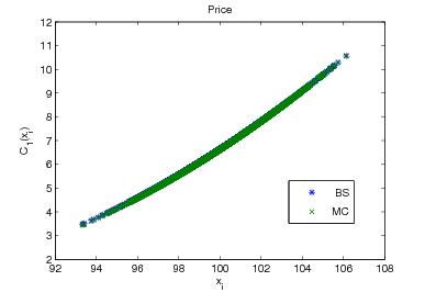
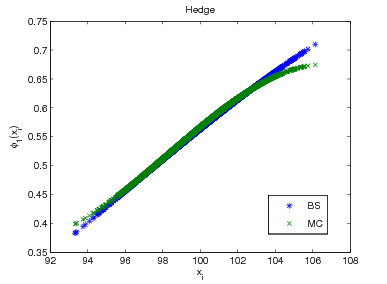
Figure 2: The results of a comparison of the actual Black-Scholes formula price and the Hedged Monte Carlo algorithm result. On the left we display the prices and on the right we display the hedge value.

Although this is a very simple text-book example, Figure 2 conveys the fact that the results are pretty accurate even for such a small number of simulations and small number of basis elements.

In the second example we check the algorithm performance of the difference of two hedgeable assets $X_{1}$ and $X_{2}$. More precisely we consider a 65 days exchange option with payoff $(X_{1,T_{F}}-X_{2,T_{F}})^{+}$. The variables $X_{1}$ and $X_{2}$ satisfy geometrical Brownian motion dynamics with $\sigma_{1}=0.3$, $\sigma_{2}=0.2$, and $r=0.05$. The analytical results are obtained using the Margrabe’s formula. In our setting this formula states that the fair price for the option is: $X_{1,0}N(d_{1})-X_{2,0}N(d_{2})$, where $N$ denotes the cumulative distribution function for a normal distribution and $d_{1,2}=\left(\ln[X_{1,0}/X_{2,0}]\pm\sigma^{2}T_{F}/2\right)/\sigma\sqrt{T_{F}}$, with $\sigma=\sqrt{0.3^{2}+0.2^{2}}$. See Musiela and Rutkowski (1997). Here, we used two monomials and $N=10000$ simulations. The results are displayed in Figure 3.

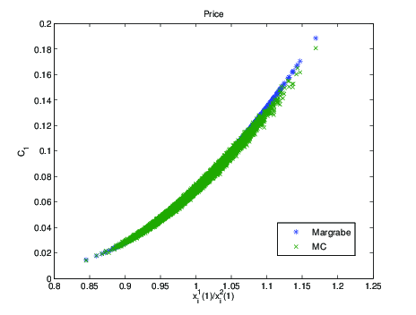
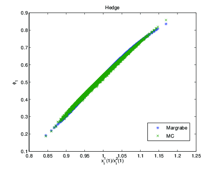
Figure 3: Results of the comparison between the HMC algorithm and the Margrabe formula.

3.2 Practical Examples

First Example

An energy company considers the optionality of starting a new project that would last for $11$ years. The project value $V_{t}$ is dependent on $12$ different underlyings. The option is exercizable every year during the first $5$ years. The company also has a trading desk that could be used for financial investment in some or all of such different assets.

The optionality was evaluated using several different sets of hedging assets. We now report on the results obtained with one hedging variable (in this example the Brent price) and considering $2000$ paths along $11$ years with a (continuously compounded annualized) interest rate $r=0.08$. We also computed examples with more hedging variables.

In Figure 4 we present the option evaluation using one hedging variable.

[width=0.7angle=0]OneSpan.png

Figure 4: Option evaluation using one hedging variable as a function of the Brent value. The difference between the project and the investment $(\mathcal{V}_{t=0}(X_{1})-K)$ is plotted in (red) crosses while the optionality $V_{t=0}(X_{1})$ is plotted with (blue) circles. Here, the investment (strike) is $K=10.89$ and the risk free interest rate $r=0.08$.

In this example the project works as a hedge towards low prices of the Brent. The fact that the intrinsic value of the project is smaller than the optionality indicates that the company should wait to start the project.

Second Example

In this example we consider a project that would run for $15$ years, an investment of $1500$ monetary units and a yearly free interest rate of $8.00\%$. The cash flows for this period are the results of an oracle that depends on a number of traded and non-tradable variables and in turn are produced by means of running different scenarios. Some of their descriptive statistics is presented in Figure 5.

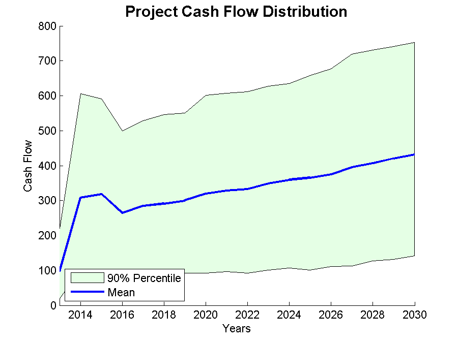
Figure 5: A description of the cash flow under the different scenarios. The lower line corresponds to the 5% quantile and top one to the 95%. The marked region indicates the 90% frequency region.

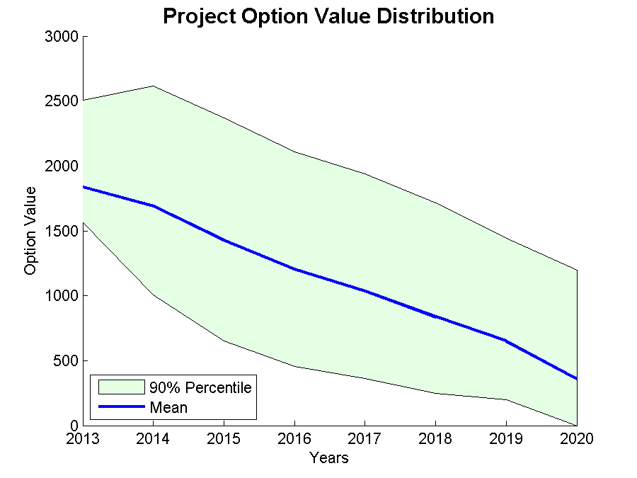
Figure 6: Value of the project optionality. The lower line corresponds to the 5% quantile and top one to the 95%. The marked region indicates the 90% frequency region.

The intrinsic values of the optionality for the different times, including the 5%, and 95% quantiles for the project value are presented in Figures 6 and 7. By applying the Hedged Monte Carlo method we compute the value of the delay optionality considering $3$ hedging variables. The project should be exercised if at a certain time and corresponding scenario the intrinsic project value is more than the delay optionality. This leads to a trigger curve that tells us for each scenario whether to invest or not (Figure 7).

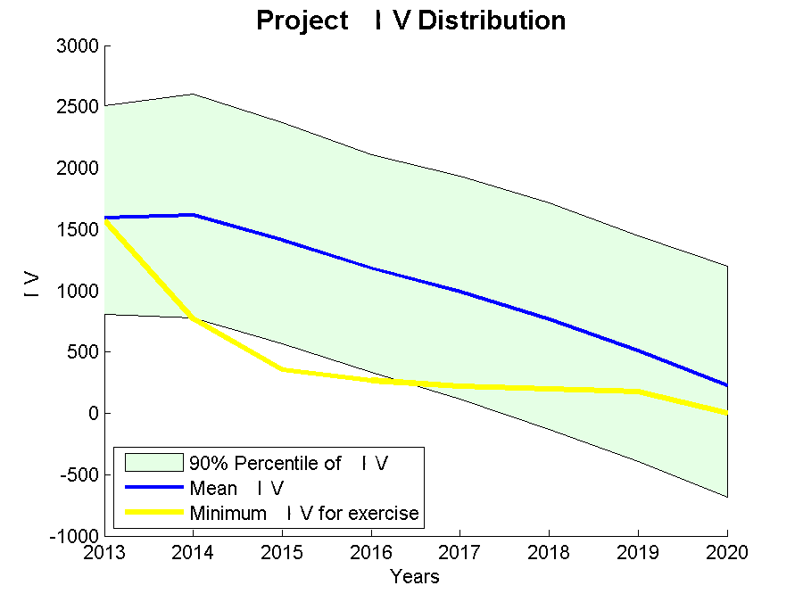
Figure 7: A description of the project Intrinsic Value (IV) statistics under the different scenarios and the minimum value for exercise. The lower line corresponds to the 5% quantile and top one to the 95%. The marked region indicates the 90% frequency region.

Third Example

Differently from the previous examples whereby the actual cash flows came from complex (black-box type) oracles, our present example concerns a fictitious project where the cash flows would come from a (fairly) simple mathematical function. It concerns an artificial potential investment on a gas propelled vehicle that could be used by an information technology company to gather geographical data and to use in their web-based advertisements. For simplicity we take the cash flow highly correlated to Google stock through the equation

$$c_{t}(X,\epsilon)=\mathsf{H}\left(aX_{1,t}-bX_{2,t}-I+\epsilon_{t}\right)\mbox{ ,}$$ (3.1)

where $X_{1}$ is the price of a Google stock, $X_{2}$ is Henry Hub (HH) gas index, $I$ is a fixed running cost, $\epsilon_{t}$ is a nonhedgeable noise. The function $H$ in our example is defined as

$$\mathsf{H}(x)=\left\{\begin{array}[]{cc}0\mbox{ ,}&x\leq 0\mbox{ ,}\\ x\mbox{ ,}&x\in(0,1)\mbox{ ,}\\ 1\mbox{ ,}&x\geq 0\mbox{ .}\end{array}\right.$$

The rationale behind $\mathsf{H}$ is to simulate the saturation given by very large values of the stock and to clip the values below zero.

We performed the data collection using publicly available data downloaded by using public domain R software . The historical results between August 19th, 2004 and November 24th, 2013 are displayed in Figure 8. We calibrated the historical log-returns of the data with a GARCH(1,1) model, and then performed a principal component analysis of the bi-dimensional innovation time series. From that we generated the simulations of future scenarios.

In this example we consider a project that would run for a maximum period of say $3$ years and the decisions could be performed monthly. The cash flows for this period are the results of the oracle described in Equation (3.1) that depends on a value of Google and HH Gas. Finally we choose an investment of $INV=3.5$ and a risk-free interest rate of $8.00\%$.

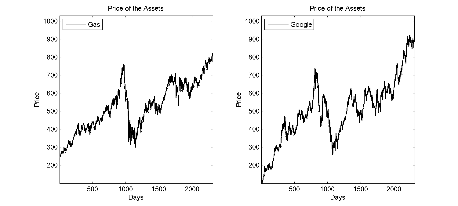
Figure 8: Time series for the assets between August 19th, 2004 and November 24th, 2013.

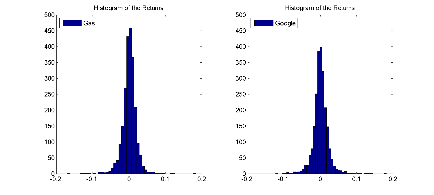
Figure 9: Histogram of the log returns for the assets between August 19th, 2004 and November 24th, 2013.

In Figure 10 we present some simulations of the assets, and in Figure 11 a description of the simulations of the cash flows by showing their mean, their quantiles.

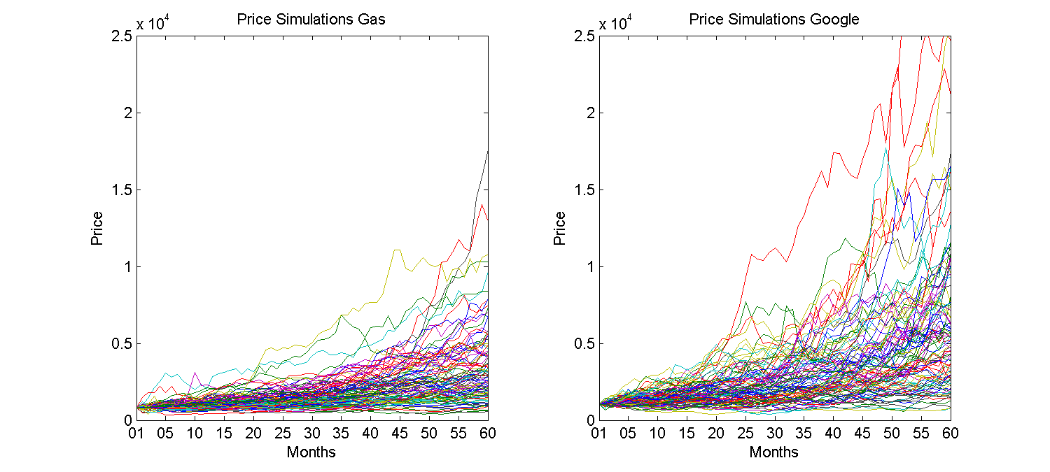
Figure 10: Asset simulations.

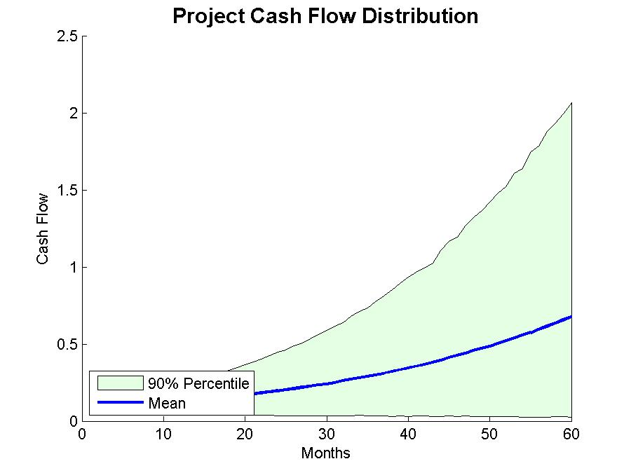
Figure 11: Cash flow simulations for the fictitious oracle described by Equation (3.1). Using the parameters value $a=1.2895\times 10^{-4}$, $b=-5.3191\times 10^{-5}$, $I=0.05$, $\varepsilon_{t}\sim\mathcal{N}(0,0.005)$

The results in Figure 13 show how the statistics of the values for the Intrinsic Value (defined as $\mathcal{V}-I$) relates to the curve of minimum value of the Intrinsic Value for exercise ($\nu_{t}$) that was calculated in the refined algorithm leading to Equation (2.1). As the time varies between $t=1$ and $t=12$, the exercise curve crosses the average of the Intrinsic Values for the different scenarios. The case of $\nu_{t}$ being smaller than the Intrinsic Value mean implies a small $Pr_{t}:=P(NPV<\nu_{t})$. These small values of $Pr_{t}$ give a good suggestion of when to invest. But the decision to invest also has to involve the option value described in Figure 12 and the expected Intrinsic Value value of Figure 13.

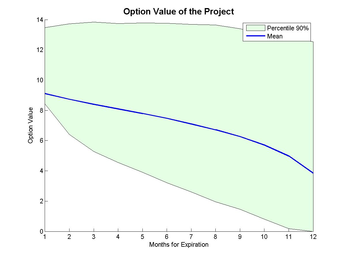
Figure 12: A description of the option value statistics under the different scenarios.

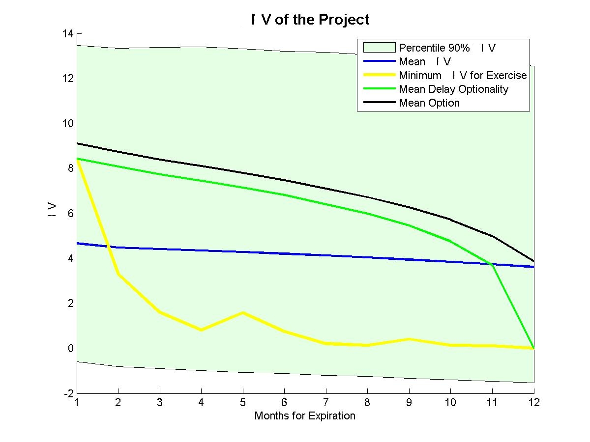
Figure 13: A description of the project Intrinsic Value statistics under the different scenarios and the minimum value for exercise.

4 Discussion and Conclusions

In this work we addressed the problem of pricing real options on projects that have their cash flow estimates based on an oracle prediction. Such oracle is typically a combination of asset prices either used for production or obtained as a result of the working project and non-traded specific variables. They can also forecast prices or demand, and they can include managerial views or other non-tradable information that impacts the project value. These prices and variables may further be processed by an optimization procedure, and this leads to the project cash flows. As discussed in the Introduction, this appears naturally in many situations, in particular for chemical or oil industries.

For such problems, we proposed a method that is based on minimizing the tracking error variance of the hedge. This can be interpreted as assuming that we are in an incomplete market and that the investor is naturally risk averse. In this context, this variance is a natural risk measure for the investor. Under this framework, we show how to price real options using the method of Potters et al (2001). This lead to a set of consistent prices that reduces to that of the Black-Scholes theory when the market is complete. The obtained price will depend on the set of assets chosen for the hedge. This is natural since companies with access to different markets and vulnerable to different scenarios can have very different values for the same project. Theoretically, one could include all hedging assets on a maximal set, but this is unfeasible from a practical point of view.

Once more, we reinforce the idea that our simulations are all done in the historical measure where the calibration of the models take place. We could also have incorporated managerial views by emphasizing scenarios that would be more likely due to management selective information. On the other extreme, even if the decision maker and the business at hand had access to a completely correlated asset that could be used to hedge the project value, among the advantages of the present approach over a risk-neutral Monte Carlo evaluation we can mention: The reduction of variance of price estimation (for the same precision the number of paths can be up to 100 times smaller). This was already documented in the original work of Potters et al (2001). The estimation of the hedging strategy, residual risk (in the form of the local variance), and possibly other risk measures (such as VaR and CVaR) at each time step.

As explained in the conclusion of the work of Grasselli (2011), it is the time flexibility itself, more than the possibility of replication, that bears the extra value of an investment opportunity. Thus, the fact that we cannot replicate the project value should not be the reason for not trying to quantify such extra value. The work of Grasselli (2011) takes the point of view of utility functions and indifference pricing. In contradistinction, here we took the point of view of minimizing risk as measured by the variance. A very natural follow up of the present work would be to compare the different approaches in the case of real world examples, such as the ones presented here. An exploration of the numerical issues related to the choice of the projection basis would also be very welcome.