Orbital signatures of Fano-Kondo line shapes in STM adatom spectroscopy

Abstract

We investigate the orbital origin of the Fano-Kondo line shapes measured in STM spectroscopy of magnetic adatoms on metal substrates. To this end we calculate the low-bias tunnel spectra of a Co adatom on the (001) and (111) Cu surfaces with our density functional theory-based ab initio transport scheme augmented by local correlations. In order to associate different $d$-orbitals with different Fano line shapes we only correlate individual $3d$-orbitals instead of the full Co $3d$-shell. We find that Kondo peaks arising in different $d$-levels indeed give rise to different Fano features in the conductance spectra. Hence the shape of measured Fano features allows us to draw some conclusions about the orbital responsible for the Kondo resonance, although the actual shape is also influenced by temperature, effective interaction and charge fluctuations. Comparison with a simplified model shows that line shapes are mostly the result of interference between tunneling paths through the correlated $d$-orbital and the $sp$-type orbitals on the Co atom. Very importantly, the amplitudes of the Fano features vary strongly among orbitals, with the $3z^{2}$-orbital featuring by far the largest amplitude due to its strong direct coupling to the $s$-type conduction electrons.

I Introduction

The Kondo effect is one of the most fascinating phenomena in condensed matter physics, occurring in a vast number of different systems (see, e.g., Ref. Hewson, 1997 and references therein), ranging from bulk metals doped with magnetic impuritiesde Haas et al. (1934); Sarachik et al. (1964); Kondo (1964) to nanoscale systems such as semiconductor quantum dotsPosazhennikova et al. (2007); Roch et al. (2008) and carbon nanotubes connected to metal leadsNygard et al. (2000); Jarillo-Herrero et al. (2005). Generally, the Kondo effect leads to the quenching of a local magnetic moment associated with localized and strongly interacting electronic states in the system by interaction with the conduction electrons. The quenching of the spin is accompanied by drastic changes in the electronic and transport properties. This strong impact on the electronic and magnetic properties of a system makes the Kondo effect an important factor for the functionality of atomic and molecular-scale electronic devices.

Since the pioneering works of Li et al.Li et al. (1998) and Madhavan et al.Madhavan et al. (1998) scanning tunneling spectroscopy (STS) has become a standard tool for probing the Kondo effect of magnetic adatoms and molecules on metallic substratesManoharan et al. (2000); Knorr et al. (2002); Nagaoka et al. (2002); Heinrich et al. (2004); Zhao et al. (2005); Crommie (2005); Iancu et al. (2006); Néel et al. (2007). The Kondo effect arises from the interaction of the magnetic moment of the adsorbate with the conduction electrons of the metal surface, and leads to the screening of the magnetic moment by formation of a total spin singlet state with the conduction electrons. The formation of the Kondo-singlet state is signaled by the appearance of a strongly renormalized quasi-particle peak at the Fermi level, the so-called Abrikosov-Suhl or Kondo resonance. In STS the appearance of the Kondo peak in the local DOS of the atom or molecule leads to a zero-bias anomaly (ZBA) in the tunnel spectra which is generally well described by a Fano line shapeFano (1961), although it has recently been found that the ZBAs are actually much better described in terms of generalized Frota line shapesPrüser et al. (2012) as the Frota function yields a much better description of the Kondo peak than the Lorentz function.Frota and Oliveira (1986); Frota (1992)

The origin of the Fano-like line shape is either understood as due to the interference of different tunneling paths - one via the strongly interacting orbitals of the magnetic atom bearing the sharp Kondo resonance, and others going directly to the substratePlihal and Gadzuk (2001); Madhavan et al. (2001); Lin et al. (2006) - or is explained in terms of tunneling into the surface aloneÚjsághy et al. (2000); Schiller and Hershfield (2000); Wahl et al. (2004); Merino and Gunnarsson (2004a, b). A recent studyBaruselli et al. (2015) combines density functional theory (DFT) with numerical renormalization group (NRG) calculations and determines the line shape by looking at energy-dependent transmission eigenvalues. Surprisingly, no systematic study of the relation between orbital symmetry of the orbital(s) bearing the Kondo resonance and the shape of the resulting Fano resonances has been conducted so far.

In this paper, we intend to close this gap by calculating the Fano line shapes corresponding to Kondo peaks appearing in different orbitals of the $3d$-shell of a magnetic atom on metal surfaces. To this end we select individual $d$-orbitals and perform ab initio quantum transport calculations augmented by local correlations for the selected $d$-orbital only. There is merit in doing so: Even in a multi-orbital situation the Kondo effect is signaled by Kondo peaks in individual $d$-orbitals, and often the Fano-Kondo feature of one $d$-orbital will be dominant in the tunnel spectrum due to different tunneling matrix elements and Kondo scales.

We choose to study Co$@$Cu(001) and Co$@$Cu(111) as our test systems, which have been extensively studied theoretically and experimentallyVitali et al. (2008); Néel et al. (2010); Merino and Gunnarsson (2004a, b); Choi et al. (2012); Knorr et al. (2002); Néel et al. (2007); Wahl et al. (2004); Lin et al. (2006); Baruselli et al. (2015). We find that Kondo peaks arising in different $d$-levels indeed give rise to different Fano features in the conductance spectra. However, temperature, effective interaction and occupancy of the $d$-orbital also play an important role. With one notable exception, a simplified two-level model consisting of the $d$-orbital bearing the Kondo resonance and one $s$- or $p$-orbital on the adatom accounts for the calculated line shapes. This shows that in these cases tunneling into substrate states only plays a minor role for determining the actual line shapes.

The paper is organized as follows: In Sec. II we briefly describe the method for calculating the zero-bias anomalies in the conductance spectra corresponding to Kondo peaks in different orbitals. In Sec. III we introduce two types of Fano line shapes: the standard one based on a Lorentzian resonance for the localized state and one based on the Frota line shape better suited for describing the Kondo resonance. In Sec. IV we present results for a Co adatom placed on a Cu(001) and a Cu(111) surface, respectively. In Sec. V we devise a simplified model capturing the essence of the different situations encountered for different orbital symmetries and discuss the obtained results in the context of this model. In Sec. VI, a more general discussion follows relating our results to other experimental and theoretical works. Finally, in Sec. VII, we conclude this work with some general remarks on the significance of our results for other atomic or molecular Kondo systems.

II Method

We consider a magnetic atom (here: Co) that is placed on a metallic substrate (here: Cu(001) or Cu(111)). A Cu STM tip is placed directly above the Co atom 6Å away so that we are in the tunneling regime. The system is divided into three parts as shown in Fig. 1: two metal leads S and T, representing the bulk electrodes connected to the substrate and STM tip, respectively, and the device region (D) which contains the magnetic atom and part of the surface and the STM tip.

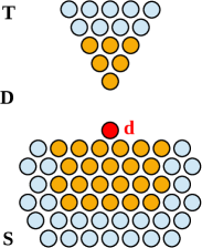
Figure 1: Schematic drawing of an STM tip probing a magnetic atom on a metal substrate. The system is separated into three parts: the device region D (gray/yellow) contains the magnetic atom (dark gray/red) hosting the $d$-orbital giving rise to the Kondo peak, and parts of the substrate and STM tip. T and S (light gray/blue) are the bulk electrodes connected to the STM tip and substrate, respectively.

We perform DFT based ab initio quantum transport calculations using the ANT.G packageJacob and Palacios (2011): The electronic structure of the D region is calculated on the level of Kohn-Sham (KS) DFT employing the LSDA functionalKohn and Sham (1965) in the SVWN parametrization Slater (1974); Vosko et al. (1980) and a minimal Gaussian basis set including the valence (4s4p3d) and outer core electrons (3s3p) of the Co and Cu atoms Hehre et al. (1969); Collins et al. (1976); Hay and Wadt (1985a); Wadt and Hay (1985); Hay and Wadt (1985b). The effect of the bulk electrodes S and T, which are modeled by Bethe latticesBethe (1935), on the electronic structure of D is taken into account via self-energies $\hat{\Sigma}_{\rm S}$ and $\hat{\Sigma}_{\rm T}$. The KS Green’s function (GF) of the D region is thus given by:

$$\hat{G}^{0}_{\rm D}(\omega)=\left((\omega+\mu)\hat{P}_{\rm D}-\hat{H}_{\rm D}^{0}-\hat{\Sigma}_{\rm T}(\omega)-\hat{\Sigma}_{\rm S}(\omega)\right)^{-1}\textrm{,}$$ (1)

where $\mu$ is the chemical potential, $\hat{P}_{\rm D}$ the projection operator onto D and $\hat{H}_{\rm D}^{0}$ is the KS Hamiltonian of the D region.

In order to capture Kondo physics, electronic correlation beyond conventional DFT have to be included. This is done by combining DFT with the one-crossing approximation (OCA)Haule et al. (2001), following the scheme developed in previous work Jacob et al. (2009); Jacob (2015). In contrast to previous work, we are interested in the Kondo signatures of specific $d$-orbitals, and not of the entire $3d$-shell.

Hence we add a Hubbard-like interaction term $\hat{\mathcal{H}}_{U}=U\hat{n}_{d\uparrow}\hat{n}_{d\downarrow}$ only to a single $d$-orbital of the Co $3d$-shell where $n_{d\sigma}$ is the number operator for the $d$-orbital and a spin $\sigma$. Since the Coulomb interaction in the correlated $d$-orbital has already been taken into account on a mean-field level in the KS-DFT calculation, a double-counting correction (DCC) term has to be subtracted from the KS Hamiltonian projected onto the $d$-orbital $\epsilon_{d}^{0}=\left\langle d\right|\hat{H}_{\rm D}^{0}\left|d\right\rangle$:

$$\epsilon_{d}=\epsilon^{0}_{d}-\epsilon_{\rm dc}\textrm{.}$$ (2)

In contrast to previous work the DCC is chosen such that a certain occupancy is achieved, i.e. for achieving particle-hole (ph) symmetry ($n_{d}=1$) we choose $\epsilon_{\rm dc}$ such that $\epsilon_{d}=-U/2$. Note that ph symmetry is only approximately achieved since the coupling of the $d$-orbital to the rest of the system (see below) is generally not ph symmetric.

The interacting $d$-orbital coupled to the electronic bath given by the rest of the system (i.e. substrate and tip) defines an Anderson impurity model (AIM)Anderson (1961). An effective description of the coupling of the $d$-orbital to the bath is given by the so-called hybridization function $\Delta_{d}(\omega)$ which can be obtained from the KS GF by

$$\Delta_{d}(\omega)=\omega+\mu-\epsilon^{0}_{d}-\left[G^{0}_{d}(\omega)\right]^{-1}\textrm{,}$$ (3)

where $G^{0}_{d}$ is the KS GF projected onto the $d$-orbital, i.e. $G^{0}_{d}=\left\langle d\right|\hat{G}^{0}_{\rm D}\left|d\right\rangle$. The imaginary part of $\Delta_{d}$ yields the broadening $\Gamma_{d}$ of the $d$-orbital due to the coupling to the rest of the system.

The AIM is now solved in the OCA.Haule et al. (2001) The solution yields the self-energy $\Sigma_{d}(\omega)$ describing the dynamic correlations of the $d$-orbital. The correlated GF of the $d$-orbital is then given by

$$G_{d}(\omega)=\left([G_{d}^{0}(\omega)]^{-1}-\Sigma_{d}(\omega)+\epsilon_{\rm dc}\right)^{-1}\textrm{.}$$ (4)

Its imaginary part yields the spectral function or LDOS of the $d$-orbital $\rho_{d}(\omega)=-{\rm Im}{}G_{d}(\omega)/\pi$. Correspondingly, we obtain the correlated GF for the D region as:

$$\hat{G}_{\rm D}(\omega)=\left([\hat{G}_{\rm D}^{0}(\omega)]^{-1}-(\Sigma_{d}-\epsilon_{\rm dc})\hat{P}_{d}\right)^{-1}\textrm{.}$$ (5)

This allows us to calculate the transmission function using the Caroli expression Caroli et al. (1971),

$$T(\omega)={\rm Tr}\left[\hat{G}_{\rm D}\hat{\Gamma}_{\rm T}\hat{G}_{\rm D}^{\dagger}\hat{\Gamma}_{\rm S}\right]$$ (6)

where the coupling matrices for the leads are defined by

$$\hat{\Gamma}_{\rm T/S}=i\left(\hat{\Sigma}_{\rm T/S}-\hat{\Sigma}_{\rm T/S}^{\dagger}\right)\textrm{.}$$ (7)

The self energies $\Sigma_{\rm T/S}$ are typically symmetric, so that the coupling matrices are twice the imaginary part of the self energies. For low temperature and small bias voltages, current and conductance can be related to the transmission function using the Landauer formulaLandauer (1957); Datta (1995). For the typical STM setup considered here most of the applied bias voltage drops at the STM tip. In that case the conductance is simply given by

$$G(V)=\frac{2e^{2}}{h}T(eV)\textrm{.}$$ (8)

We note that the use of the Landauer formula for the conductance is justified in the limit of small bias voltages compared to the Kondo temperature. In this limit transport occurs via the Kondo resonance and thus is essentially one-body like (apart from renormalization) and phase coherent so that the full non-equilibrium expression for transport through an interacting region given by Meir-Wingreen reduces to the simpler Landauer result.Meir and Wingreen (1992) For larger bias voltages, deviations from the Landauer result can occurHettler et al. (1998); Balseiro et al. (2010); Roura-Bas (2010), and one would have to make use of the Meir-Wingreen equationMeir and Wingreen (1992) which requires the solution of the AIM out of equilibrium.

III Fano-Lorentz and Fano-Frota line shapes

Fano line shapes or resonances, originally introduced by Fano in the context of autoionization and elastic electron scattering by heliumFano (1961), generally arise in resonant scattering processes due to quantum interference between a quasi discrete resonant state and a broad background continuum. The interference leads to an asymmetric line shape in the scattering cross section at energies close to the resonance energy that is well described by the Fano function

$$f(\epsilon)\propto\frac{(q+\epsilon)^{2}}{\epsilon^{2}+1}\textrm{,}$$ (9)

where the parameter $q$ controls the shape of the Fano function, and $\epsilon$ is the energy with respect to the resonant level. Eq. 9 can also be obtained from the complex representation of a Lorentzian multiplied by a phase factor $e^{i\phi_{q}}$

$$\rho_{\rm FL}(\omega)={\rm Im}\left[e^{i\phi_{q}}\left(\frac{A}{\omega-\omega_{0}+i\Gamma}\right)\right]+\rho_{0}\textrm{,}$$ (10)

where $A$ is the amplitude, $\Gamma$ is the half-width of the Lorentzian, $\omega_{0}$ the resonance energy and $\rho_{0}$ a constant offset. Using $q=\tan(\phi_{q}/2)$, $\epsilon=(\omega-\omega_{0})/\Gamma$ and some algebra, this Fano-Lorentz (FL) line shape can be shown to be equivalent to the original Fano formula (see the Appendix):

$$\rho_{\rm FL}(\omega)=\frac{A}{\Gamma}\left(\frac{(q+\epsilon)^{2}}{\epsilon^{2}+1}-1\right)\frac{1}{1+q^{2}}+\rho_{0}\textrm{.}$$ (11)

STM spectroscopy of Kondo impurities presents a similar situation: The STM tip probes the continuous conduction electron density of states which interacts with the Kondo resonance at the Fermi level. The interference of different tunneling paths then leads to Fano-type line shapes in the conductance spectra. Assuming a Lorentzian form for the Kondo resonance naturally leads to Fano-Lorentz line shapes given by (11). However, in Refs. Frota and Oliveira, 1986; Frota, 1992 Frota showed that the Kondo peak is actually better described by a line shape now known as a Frota line shape:

$$\rho_{\rm Frota}(\omega)=A\cdot{\rm Re}\left[\sqrt{\frac{i\Gamma_{F}}{\omega-\omega_{0}+i\Gamma_{F}}}\right]\textrm{.}$$ (12)

where the Frota parameter $\Gamma_{\rm F}$ is related to the actual half-width $\Gamma$ of the resonance by $\Gamma\sim 2.54\,\Gamma_{\rm F}$. $A$ is the amplitude and $\omega_{0}$ the position of the Frota resonance. In analogy with Eq. (10) we define a Fano-Frota (FF) line shape as a generalized Frota curve Prüser et al. (2011) for describing the transmission function close to the Kondo resonance

$$T_{\rm FF}(\omega)=-A\cdot{\rm Re}\left[e^{i\phi_{q}}\sqrt{\frac{i\Gamma_{\rm F}}{\omega-\omega_{0}+i\Gamma_{\rm F}}}\right]+T_{0}\textrm{.}$$ (13)

The phase $\phi_{q}$ has the same meaning in the Lorentz and in the Frota case: A value of $\phi_{q}=0$ leads to a dip, $\phi_{q}=\pi$ to a peak and $\phi_{q}=\pi/2$ to a symmetric Fano line shape. In Fig. 2, we compare Fano-Frota and Fano-Lorentz features, choosing identical amplitudes and half-widths. Note that for the same half-width Frota line shapes have a slower decay than the Lorentzian ones.

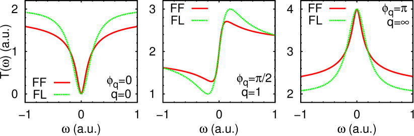
Figure 2: Comparison of Fano-Frota and Fano-Lorentz line shapes for different values of the $q$ parameter but for identical amplitudes and half-widths.

In Fig. 3, we show FL and FF fits to the Kondo peak (left) in the calculated spectral function $\rho_{d}(\omega)$ and the corresponding Fano line shape (right) in the calculated transmission function $T(\omega)$ for the case of the $z^{2}$-orbital for the Co on Cu(001) system, discussed in detail in the following section. For both spectral and transmission function, the resonance center is well-described by FF and FL fits. However, only the FF fit yields an accurate description of the flanks and the long range decay. In the following, we will therefore use Eqn. 13 to fit transmission functions.

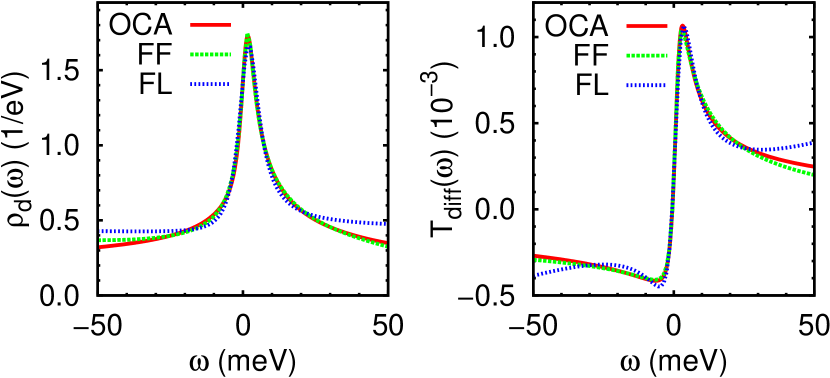
Figure 3: Fano-Lorentz (FL) and Fano-Frota (FF) fits of the impurity spectral function $\rho_{d}(\omega)$ (left) and the transmission function $T(\omega)$ (right) for $z^{2}$-orbital, Co@Cu(001), $U=2$ eV and $\epsilon_{d}=-1.0$ eV. See Sec. IV.1 for details.

IV Results

IV.1 Co adatom on Cu(001) surface

The system under consideration is shown in the left panel of Fig 4. A Cobalt atom is deposited at the hollow site of a Cu(001) surface. The Cu(001) surface is modeled by three Cu slabs of 36, 25 and 16 atoms, respectively, which are embedded into a Bethe lattice to describe the infinitely extended surface. We model the STM tip by a small pyramid of Cu atoms grown in the (001) direction, also embedded into a Bethe lattice. The tip is placed directly above the Co atom in a distance of 6Å, so that the system is in the tunneling regime.

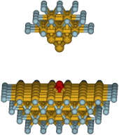
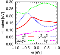
Figure 4: Left: Geometry of the Co atom deposited on a Cu(001) surface; dark gray/red: Co, gray/yellow: Cu, light gray/blue: Bethe lattice. Right: Imaginary part of the hybridization function for the Co $3d$ shell.

As explained in Sec. II we now compute the hybridization functions of the Co $3d$-orbitals (see right panel of Fig. 4). The four-fold symmetry of the Cu(001) surface leads to a splitting into four groups. The $xz$- and $yz$-orbitals are degenerate (in the following, results for the $yz$-orbital are omitted) and exhibit the strongest hybridization at the Fermi level. The hybridization functions of $z^{2}$ and $x^{2}$-$y^{2}$ have comparable values around the Fermi level. The $xy$-orbital has the lowest hybridization in the displayed energy window. All hybridization functions show a moderate energy dependence. Note that the hopping between different Co $3d$ orbitals is zero, i.e. they do not couple to each other on the single-particle level.

While the hybridization function is calculated ab initio, the Coulomb interaction $U$ is used as a parameter that allows us to tune the Kondo coupling strength and explore the effect of the width of the Kondo peak on the transmission line shape. But in order to have an estimate of the magnitude, we have also calculated $U$ ab initio for each of the $d$-orbitals by constrained RPA calculations as described in Ref. Jacob (2015). We find values for $U$ ranging from 1.8 eV to 2.6 eV. Accordingly, we choose the $U$ parameters to vary between 2 eV and 3 eV.

The hybridization functions from Fig. 4 together with the energy level $\epsilon_{d}$ and the effective Coulomb interaction $U$ define an AIM which is solved in the OCA Haule et al. (2001). It is a known issue of OCA that at too low temperatures (1-2 orders of magnitude below $T_{K}$) it gives rise to spurious non-Fermi liquid behavior and related artifacts in the impurity spectral function, leading to an overestimation of the height of the Kondo peak and an unphysical self-energy with positive imaginary part Costi et al. (1996). We circumvent this problem by lowering the temperature only to the point where the imaginary part of the self-energy becomes zero. At this point Fermi liquid behavior is obeyed, and the unitary limit of the Kondo peak is exactly recovered.

Figure 5: Impurity spectral functions for the $z^{2}$ orbital of Co$@$Cu(001) for different Anderson impurity model parameters $U$, $\epsilon_{d}$.

Fig. 5 shows impurity spectral functions $\rho_{d}(\omega)$ of the $z^{2}$-orbital for different values of the AIM parameters $\epsilon_{d}$ and $U$. For $\epsilon_{d}=-U/2$ (red solid and blue dotted curves) we have approximate particle-hole symmetry: the Kondo peak is centered close to, but slightly above the Fermi level. Note that exact particle-hole symmetry is not achieved because of the non-constant hybridization function. As expected, when $U$ is increased the Kondo temperature and hence the width of the Kondo peak decrease strongly. On the other hand detuning the system from particle-hole symmetry by shifting $\epsilon_{d}$ leads to a strong increase of the Kondo temperature due to charge fluctuations (green dashed, magenta dashed-dotted curves).

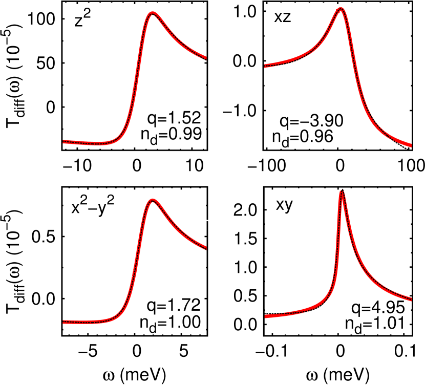
Figure 6: Transmission functions for different $d$-orbitals of Co$@$Cu(001). Coulomb repulsion $U=2$ eV, and energy level $\epsilon_{d}=-1$ eV (approximate particle-hole symmetry). The red continuous curves show the calculated transmission, the black dashed curves Fano-Frota fits. The transmission background has been subtracted.Note (2)

We now calculate the correlated transmission functions for Kondo peaks in different $d$-orbitals. Fig. 6 shows transmission line shapes for different $d$-orbitals for $U=2$ eV and $\epsilon_{d}=-1.0$ eV. In order to make the features more clearly visible, here and in the following the transmission background was subtracted. We find that the line shapes are indeed different for each orbital. We observe approximately antisymmetric Fano line shapes ($q\approx 1$) for $z^{2}$ and $x^{2}-y^{2}$, and more peak-like feature ($q\gg 1$) for $xz$ and $xy$. In order to quantitatively describe the line shapes, we perform Frota fits to determine the $q$ parameter and width of the line shapes, as explained before in Sec. III. The $z^{2}$ and $x^{2}-y^{2}$ orbitals have comparable $q$ values of 1.52 and 1.72, respectively. For $xz$, $q$ becomes negative ($-3.9$) and for $xy$ we find the most pronounced peak with $q=4.95$. The width of the Fano features differs significantly, and in accordance with their hybridization strength at the Fermi level. Note that a feature with a very small width, as e.g., in the case of $xy$, might never be observed in an actual experiment, because of the Kondo temperature being much too low and because of limited resolution.

We now vary the Coulomb repulsion $U$ and introduce charge fluctuations by shifting the $d$-level position $\epsilon_{d}$, as can be seen in Fig. 7. When varying $U$, but maintaining particle-hole symmetry, the actual shape of the transmission features is only weakly affected, while the widths of the features change strongly, as has already been seen and discussed for the spectral functions in Fig. 5. When introducing charge fluctuations, the Kondo peak becomes asymmetric (see Fig. 5). This asymmetry is also reflected in the transmission line shapes. We find that the $q$ parameter consistently increases when $\epsilon_{d}$ is shifted downwards. For positive $q$ ($z^{2}$, $x^{2}-y^{2}$, $xy$) lowering $\epsilon_{d}$ makes the line shapes more peak-like, while for negative $q$ ($xz$), lowering $\epsilon_{d}$ leads to more dip-like line shapes.

Hence while the choice of AIM parameters $U$ and $\epsilon_{d}$ does affect the transmission line shapes to some degree, it does not completely change its symmetry. For example, the sign of the $q$ factor does not change.

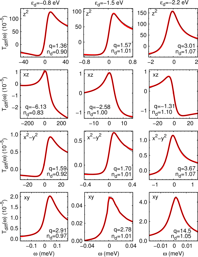
Figure 7: Transmission functions for different $d$-orbitals of Co$@$Cu(001). Coulomb repulsion $U=3$ eV, vary occupation by shifting $\epsilon_{d}$. The red continuous curves show the calculated transmission, the black dashed curves Fano-Frota fits. The transmission background has been subtracted.Note (2)

While the signal width is determined by the hybridization and choice of AIM parameters exclusively, the signal amplitude decisively depends on the system geometry. Because we chose the $z$-axis as our transport direction, a Kondo peak in the $z^{2}$-orbital results in a much more dominant feature compared to the remaining $d$-orbitals, as can be seen in Figs. 6 and 7. Hence if there is a Kondo peak in the $z^{2}$-orbital, the corresponding Fano feature will dominate in the transmission regardless of what happens in the other orbitals. Also Fano features due to Kondo peaks in orbitals other than the $z^{2}$-orbital might be difficult to discern from the background if the background dispersion is strong compared to the Fano amplitudes. This statement remains true even if the STM tip is shifted laterally by moderate distances of a few Å. Although tunneling into orbitals other than $z^{2}$ becomes more favorable upon a lateral shift of the tip, the feature due to the Kondo peak in the $z^{2}$ remains the most dominant one.

IV.2 Co adatom on Cu(111) surface

The next system we focus on is a Cobalt atom, deposited at the ’hcp’ hollow site of a Cu(111) surface, as can be seen in the left panel of Fig. 8. The surface is modeled by three Cu slabs of 27, 37 and 27 atoms, respectively, which are connected to a Bethe lattice. The tip is described by a Cu(111) pyramid, consisting of 10 copper atoms, also connected to a Bethe lattice. The threefold symmetry splits the five orbitals of the Co $3d$-shell into three groups: the non-degenerate $z^{2}$-orbital ($m=0$) and two doubly degenerate groups, one with $m=\pm 1$ ($xz$- and $yz$-orbitals) and one with $m=\pm 2$ ($xy$- and $x^{2}-y^{2}$-orbitals). The right panel of Fig. 8 shows the hybridization functions for each of the three groups. The group with the $xz$- and $yz$-orbitals exhibit the strongest hybridization at the Fermi level, the group with the $x^{2}-y^{2}$- and $xy$-orbitals the weakest.

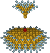
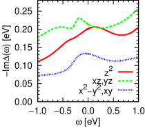
Figure 8: Left: Geometry of the Co atom deposited on a Cu(111) surface; dark gray/red: Co, gray/yellow: Cu, light gray/blue: Bethe lattice. . Right: Imaginary part of the hybridization function of the Co $3d$-shell.

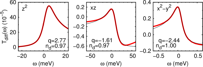
Figure 9: Transmission functions for different $d$-orbitals of Co$@$Cu(111). Coulomb repulsion $U=2$ eV, $\epsilon_{d}=-1.0$ eV. The red continuous curves show the calculated transmission, the black dashed curves Fano-Frota fits. The transmission background has been subtracted.Note (2)

We proceed as described in the previous section and calculate transmission functions for the $d$-orbitals of Co$@$Cu(111), assuming a Coulomb repulsion of $U=2~{}eV$ and (approximate) particle-hole-symmetry $\epsilon_{d}=-1.0$ eV (Fig. 9). Again, we find different line shapes for each orbital. The $z^{2}$ orbital gives the most peak-like transmission feature with $q=2.77$, for $x^{2}-y^{2}$ we observe a transmission peak with a negative $q=-2.44$. The $xz$-orbital results in a Fano-type feature with $q=-1.61$. The widths of the transmission features differ considerably, with the $xz$- and $yz$-orbitals having the largest width, and the $xy$- and $x^{2}-y^{2}$-orbitals the lowest. The $z^{2}$-orbital again has the highest signal amplitude, as it couples strongly to the tip conduction electrons.

In Fig. 10, we calculate line shapes for different AIM parameters $U$ and $\epsilon_{d}$. We observe a similar behavior as for Co$@$Cu(001). When staying in the particle-hole symmetric case and increasing $U$ (middle column of Fig. 10), the line shapes remain similar, with slightly increased $q$ values. We introduce charge fluctuations by shifting the position of $\epsilon_{d}$ (left and right column of Fig. 10). The $q$ parameter increases when moving $\epsilon_{d}$ to lower energies. For positive $q$ values, as for $z^{2}$, this leads to more peak-like line shapes, while for negative $q$ values, as for $xz$ and $x^{2}-y^{2}$, it leads to more fano- or dip-like line shapes. The only exception to this behavior occurs for the $xz$ orbital, $U=3$ eV and $\epsilon_{d}=-0.8~{}eV$. It has a very high Kondo temperature and equivalently wide Fano feature, and the Fano-Frota fit fails for negative energies. This suggests that the Fano line shape overlaps with other transmission features that alter the final line shape.

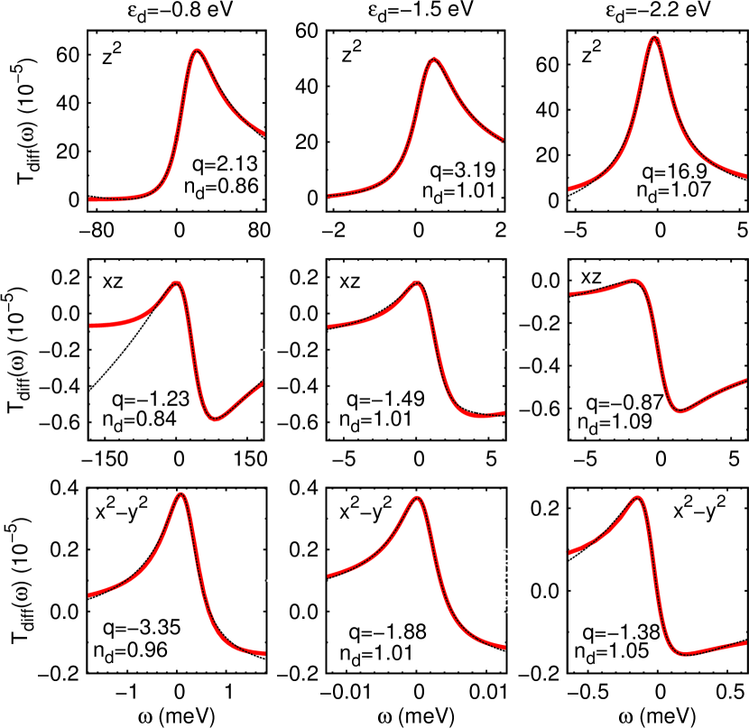
Figure 10: Transmission functions for different $d$-orbitals of Co$@$Cu(111). Coulomb repulsion $U=3$ eV, vary occupation by shifting $\epsilon_{d}$. The red continuous curves show the calculated transmission, the black dashed curves Fano-Frota fits. The transmission background has been subtracted.Note (2)

IV.3 Temperature dependence and the occurrence of dips

The results presented so far are for the case of $T\rightarrow 0$ (according to the criterion discussed in Sec. IV.1). We now study the temperature dependence of two line shapes: One tending towards a peak ($q>1$) and one tending towards a dip ($q<1$). We pick the $xz$ orbital of Co$@$Cu(111), $U=3$ eV, $\epsilon_{d}=-1.5$ eV ($q=-1.49$) and $\epsilon_{d}=-2.2$ eV ($q=-0.87$), respectively. The top row of Fig. 11 shows the evolution of the aforementioned two line shapes. For increasing temperature, the signal amplitude diminishes, while its width grows. The peak does not decay symmetrically. The ’peak’ component of the Fano feature decays faster than the ’dip’ component of the feature, so that, in both cases, the feature as a whole becomes increasingly dip-like with increasing temperature. In order to quantify that, we perform Fano-Frota fits and calculate the $q$ parameter. We find that the $q$ parameter decreases considerably when temperature is rising, irrespective if the feature tends more towards peak or dip in the $T\rightarrow 0$ case.

Figure 11: Temperature dependence of two different line shapes for Co$@$Cu(111), $xz$, $U=3$ eV, $\epsilon_{d}=-1.5$ eV and $\epsilon_{d}=-2.2$ eV, respectively. Top: Transmission. Bottom: $q$ parameter; the lines are a guide for the eye.

V A simplified model

The interference mechanism leading to different Fano line shapes still is a matter of discussion Újsághy et al. (2000); Schiller and Hershfield (2000); Plihal and Gadzuk (2001); Madhavan et al. (2001); Wahl et al. (2004); Luo et al. (2004); Merino and Gunnarsson (2004a, b); Luo et al. (2004); Lin et al. (2006); Žitko and Pruschke (2010). We expand on this discussion by introducing a simple model that allows us to determine transmission line shapes from ab initio parameters. Fig. 12 shows a schematic drawing of our model system. The central assumption is that the quantum interference primarily occurs on the magnetic adatom, namely between one $s$-type and/or $p$-type level (in the following, we will simply call it the conduction level $c$) and the correlated $d$-level. Both levels are in contact to the tip T and the surface S, and the respective interactions are taken into account by coupling matrices $\Gamma_{\rm{T/S}}$. As a second central assumption we neglect the direct tunneling from the tip to the surface.

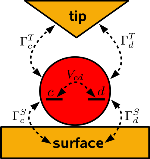
Figure 12: Sketch of the simplified model. The effective atom A is described by the correlated $d$-level and one conduction electron level $c$, in contact with the surface and the tip.

The starting point of our model is the correlated Green’s function of the effective atom comprising the conduction $c$-level and the correlated $d$-level of the magnetic atom.

$$G_{\rm{A}}(\omega)=\left(\omega\hat{P}_{\rm A}-\hat{H}_{\rm A}-\hat{\Delta}(\omega)-\Sigma_{d}(\omega)\hat{P}_{d}\right)^{-1}$$

$$=\begin{pmatrix}\omega-\epsilon_{c}-\Delta_{c}(\omega)&\quad-V_{cd}-\Delta_{cd}(\omega)\\ -V_{dc}-\Delta_{dc}(\omega)&\quad\omega-\epsilon_{d}-\Delta_{d}(\omega)-\Sigma_{d}(\omega)\end{pmatrix}^{-1}$$

$\hat{P}_{\rm A}$ is a projector onto the effective atom A, while $\hat{P}_{d}$ projects onto the $d$-level only. All parameters can either be extracted from the KS-calculation ($\epsilon_{d}$, $\epsilon_{c}$, $V_{cd}$, $\hat{\Delta}(\omega)$) or from the OCA-calculation ($\Sigma_{d}(\omega)$), while the chemical potential has been set to zero $\mu=0$. The diagonal elements of the hybridization function $\hat{\Delta}(\omega)$ lead to a shift (real part) of the level position of $\epsilon_{c}$ and $\epsilon_{d}$, respectively, and yield an effective level broadening (imaginary part). Also note that the hybridization function has off-diagonal components $\Delta_{cd}(\omega)=\Delta_{dc}(\omega)$, which can be understood as an additional hopping between the $c$- and $d$-level mediated by hoppings via the substrate, to give a total effective coupling of $\tilde{V}_{cd}=V_{cd}+\Delta_{cd}$. The coupling matrices $\Gamma_{\rm{S/T}}(\omega)$ necessary for calculating the transmission function by Eq. 6 can be obtained by decomposing the hybridization function into a tip ($\Delta_{\rm{T}}(\omega)$) and a surface ($\Delta_{\rm{S}}(\omega)$) component and taking the imaginary parts, i.e. $\Gamma_{\rm{S/T}}(\omega)=-2\,{\rm Im}\,\Delta_{\rm{S/T}}(\omega)$.

For the conduction level $c$ of the effective atom we choose the $s$- or $p$-orbital that couples to the correlated $d$-orbital. In the case of the (001) and the (111) substrates the $z^{2}$-orbital couples to the $s$- as well as the $p_{z}$-orbital. In this case we apply a unitary transformation in the subspace of the $s$- and $p_{z}$-orbitals such that the $z^{2}$-orbital decouples completely from one of the orbitals in the new basis. The $sp_{z}$-hybridized orbital coupling to the $z^{2}$ is then found to be the linear combination $\left|sp_{z}\right\rangle\propto\tilde{V}_{sz^{2}}\left|s\right\rangle+\tilde{V}_{p_{z}z^{2}}\left|p_{z}\right\rangle$ where $\tilde{V}_{sz^{2}}$ and $\tilde{V}_{p_{z}z^{2}}$ are the effective hoppings of the $z^{2}$-orbital with the $s$- and $p_{z}$-orbitals, respectively. On both surfaces, the $xz$-orbital couples to $p_{x}$ and the $yz$-orbital to $p_{y}$. For the (001) surface both the $x^{2}-y^{2}$- and the $xy$-orbitals do not interact with any of the $s$- or $p$-orbitals on the atom, while on the (111) surface, they do interact with the $p_{y}$- and $p_{x}$-orbitals, respectively.

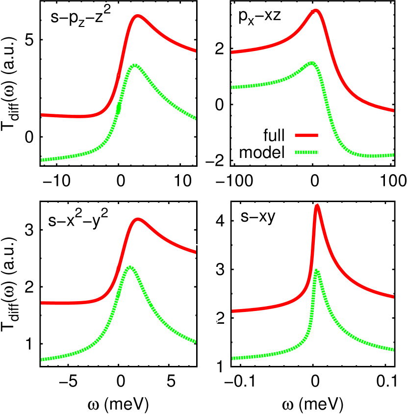
Figure 13: Transmissions calculated ab initio with the ANT.G package (see Sec. IV) and for the simplified model; Co$@$Cu(001), $U=2$ eV, $\epsilon_{d}=-1$ eV. The transmission functions are rescaled and offset for better visibility.

In Fig. 13 and 14, we compare line shapes calculated for the simplified model with the full ab initio results from Sec. IV. For the Co$@$Cu(001) surface, the simplified model consisting of the $z^{2}$-orbital and the $sp_{z}$-hybridized orbital reproduces the line shape of the $z^{2}$-orbital quite well. Only the peak character is slightly overestimated. In the case of the $xz$-orbital the line shape of the simplified model including the $p_{x}$-orbital is in excellent agreement with that of the full ab initio calculation. For the $x^{2}-y^{2}$-orbital the agreement between the simplified model and the full calculation is not as good. As stated before this orbital does not interact with any $s$- or $p$-orbital on the Co atom. Hence the transmission of the simplified model reproduces simply the Kondo peak in the spectral function since no interference is taking place. On the other hand the full transmission shows a somewhat asymmetric Fano feature ($q\approx 1.7$) indicating that interference with some substrate state(s) must take place, which is not included in the model. Finally, for the $xy$-orbital we find very good agreement between the simplified model and the full calculation. The line shape in both calculations simply reproduces the Kondo peak in the spectral function of the $xy$-orbital indicating the absence of any interference effects between this $d$-level and $s$- and $p$-levels on the atoms as well as substrate states.

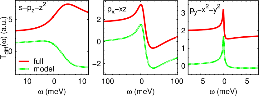
Figure 14: Transmissions calculated ab initio with the ANT.G package (see Sec. IV) and for the simplified model; Co$@$Cu(111), $U=2$ eV, $\epsilon_{d}=-1$ eV. The transmission functions are rescaled and offset for better visibility.

We find a somewhat similar picture for Co$@$Cu(111). For the $xz$-orbital the model including the interaction with the $p_{x}$-orbital gives a line shape in excellent agreement with the full calculation. Also for the $x^{2}-y^{2}$ the simplified model including the $p_{y}$-orbital on the atom reproduces the line shape of the full calculation very well. However, in the case of the $z^{2}$-orbital the simplified model including the $sp_{z}$-hybridized orbital fails quite badly in reproducing the line shape of the full calculation. Apparently, interference with tunneling paths to substrate states play an important role here.

VI Discussion

For Co$@$Cu(001), we found transmission line shapes ranging from asymmetric Fano features with positive ($z^{2}$, $x^{2}-y^{2}$) and negative ($xz$) $q$ values to a more peak-like feature ($xy$). The line shapes are determined by the interference of different tunneling paths. Our simplified model calculations indicate that for $z^{2}$ and $xz$ the interference takes place on the adatom between the correlated $d$-level and the non-interacting $sp$-levels coupling to the $d$-orbital. For the $xy$-orbital, no interference occurs between the conduction and impurity tunneling channels. Hence one directly observes the shape of the Kondo peak in the transmission. On the other hand, for the $x^{2}-y^{2}$-orbital, the interference mechanism probably involves the Cu substrate states which are not captured by the simplified model. Experimentally, asymmetric Fano line shapes were reported with $q\sim 1.1-1.2$ in the tunneling regimeKnorr et al. (2002); Néel et al. (2007). The measured line shapes are comparable to the features we found both in the $z^{2}$- and $x^{2}-y^{2}$-orbitals (see Figs. 6 and 7), although the $z^{2}$-orbital yields a slightly better agreement. Better agreement with experiment can surely be achieved by adjusting the Anderson model parameters and fitting the calculated spectra with the experimental ones. We would like to stress though that finding good agreement with experiment is not the primary goal of this work, but rather to demonstrate how different orbital symmetries give rise to different Fano-Kondo line shapes. A recent study by one of usJacob (2015) found an underscreened Kondo effect for Co$@$Cu(001), where the $z^{2}$ and $x^{2}-y^{2}$ are nearly half filled, but only the $z^{2}$ orbital is Kondo screened at finite temperatures due to its higher Kondo temperature. Ref. Baruselli et al., 2015 comes to similar conclusions, finding a Kondo peak in the $z^{2}$-orbital with $q=1.2$ in the tunneling regime and explaining it due to the interference of the $z^{2}$- with the $s$-orbital.

For Co$@$Cu(111), we found asymmetric to peak-like Fano line shapes with positive ($z^{2}$) and negative ($xz$, $x^{2}-y^{2}$) $q$ values. For the latter two, we can understand the tunneling interference in terms of the model presented in the previous section. The interference occurs on the magnetic atom, between the conduction electron channel, modeled by one of the $p$-orbitals, and the respective $d$-level. For $z^{2}$, which is interacting with the $sp_{z}$ hybridized level, our model fails, indicating that interference with substrate states plays an important role here.

Experimentally, dips were reported with $q$ values close to zeroKnorr et al. (2002); Manoharan et al. (2000); Vitali et al. (2008) which does not seem to agree with any of the calculated line shapes. The $z^{2}$-orbital, aligned in the transport direction, again shows the strongest signal, but is rather peak-like. The closest candidate to a dip-like line shape is the $xz$-orbital, particularly when increasing the occupancy relative to half-filling by moving the $d$-level position downwards in energy (see Fig. 10). In Sec. IV.3, we studied its temperature dependence, and found that the line shape became increasingly dip-like when increasing temperature. However, note that in our calculations for the $xz$-orbitals we find $q<0$ while in experiment $q$ is always positive.

Probably, the surface state of the Cu(111) surfaceCrommie et al. (1993) plays an important role for determining the line shape Manoharan et al. (2000); Bogicevic et al. (2000); Merino and Gunnarsson (2004b); Lin et al. (2006) since its tunneling amplitude may be twice as strong compared to tunneling into bulk statesJeandupeux et al. (1999). However, our embedded cluster calculation probably does not capture the surface state properly. The importance of the surface state for reproducing the correct line shape in the Co$@$Cu(111) system is also stressed in Ref. Baruselli et al., 2015 where the surface state is not properly captured and the correct $q$ value could not be reproduced either.

VII Conclusions

In summary, we have calculated the orbital signatures of Kondo peaks in the STM spectra of transition metal adatom systems, namely Co$@$Cu(001) and Co$@$Cu(111). Our calculations show that the measured line shapes allow us to draw some conclusions on the $d$-orbital(s) involved in the Kondo effect since the line shape depends to a large extent on the coupling of the $d$-orbital to the $sp$-orbitals on the adatom, which in turn is determined by the orbital symmetry. However, also temperature, effective interaction $U$ and in particular the occupancy of the $d$-orbital have a strong influence on the actual line shapes. Also, if multi-orbital effects are important for the actual shape of a Fano-Kondo feature, this approach per se is not appropriate. Nevertheless, even in the case of a multi-orbital Kondo effect, often one orbital will be dominant in the tunnel spectra. In fact if a Kondo resonance forms in the $z^{2}$-orbital, the corresponding Fano feature will be dominant in the tunnel spectrum for the typical case of an $s$-type STM tip, so that Kondo features coming from other $d$-orbitals are likely not visible. These results are also relevant for STS of transition metal complexes on metallic substrates Jacob et al. (2013); Kügel et al. (2014); Karan et al. (2015), maybe even more so since tunneling into surface states is less important there.

We stress that the here developed method can in principle also be applied to the contact regime. However, unlike in the tunneling case, in the contact regime the voltage can no longer be assumed to mainly drop between tip and adatom. Rather, the voltage drop will distribute in some way over the contact according to the actual geometry of the contact region Karan et al. (2015), and needs to be calculated or estimated. Moreover, the actual contact geometry is probably also relevant for the coupling between $d$-orbitals and conduction electrons and thus also has a strong influence on the line shapes. Therefore possible contact geometries need to be explored and relaxed with some care.

Based on our results, we propose a poor man’s method to obtain information on the orbital(s) involved in the Kondo effect measured in an actual experiment solely on the basis of a density functional theory calculation of the system: by tailoring an appropriate self-energy for each orbital such that the width of the resulting Kondo peak in that orbital reproduces the width of the measured Fano-Kondo line shape, one can calculate the corresponding line shapes and compare to experiment.

Appendix A Complex and real Fano line shapes

Here we derive the real Fano line shape given by Eq. (11) from its complex representation in Eq. (10):

$$\rho_{\rm FL}(\omega)={\rm Im}\left[e^{i\phi_{q}}\left(\frac{A}{\omega-\omega_{0}+i\Gamma}\right)\right]$$ (15)

Introducing the abbreviation $\epsilon=(\omega-\omega_{0})/\Gamma$, we have

$$\rho_{\rm FL} = \frac{A}{\Gamma}\cdot{\rm Im}\left[\left(\cos(\phi_{q})+i\sin(\phi_{q})\right)\frac{\epsilon-i}{\epsilon^{2}+1}\right]$$

$$= \frac{A}{\Gamma}\left[\frac{-\cos(\phi_{q})+\epsilon\sin(\phi_{q})}{\epsilon^{2}+1}\right]$$

$$= \frac{A}{\Gamma}\left[\frac{-\cos^{2}(\frac{\phi_{q}}{2})+\sin^{2}(\frac{\phi_{q}}{2})+2\epsilon\sin(\frac{\phi_{q}}{2})\cos(\frac{\phi_{q}}{2})}{\epsilon^{2}+1}\right]$$

$$= \frac{A}{\Gamma}\left[\frac{-1+\tan^{2}(\frac{\phi_{q}}{2})+2\epsilon\tan({\frac{\phi_{q}}{2}})}{\epsilon^{2}+1}\right]\cos^{2}\left(\frac{\phi_{q}}{2}\right)$$

Defining $q\equiv\tan(\phi_{q}/2)$, we arrive at

$$\rho_{\rm FL}=\frac{A}{\Gamma}\left[\frac{(q+\epsilon)^{2}}{\epsilon^{2}+1}-1\right]\frac{1}{1+q^{2}}$$ (16)

which is the same as Eq. (11).

References

- Hewson (1997) A. Hewson, The Kondo Problem to Heavy Fermions, edited by D. Edwards and D. Melville (Cambridge University Press, Cambridge, 1997).
- de Haas et al. (1934) W. de Haas, J. de Boer, and G. van dën Berg, Physica 1, 1115 (1934).
- Sarachik et al. (1964) M. P. Sarachik, E. Corenzwit, and L. D. Longinotti, Phys. Rev. 135, A1041 (1964).
- Kondo (1964) J. Kondo, Progress of Theoretical Physics 32, 37 (1964).
- Posazhennikova et al. (2007) A. Posazhennikova, B. Bayani, and P. Coleman, Phys. Rev. B 75, 245329 (2007).
- Roch et al. (2008) N. Roch, S. Florens, V. Bouchiat, W. Wernsdorfer, and F. Balestro, Nature 453, 633 (2008).
- Nygard et al. (2000) J. Nygard, D. H. Cobden, and P. E. Lindelof, Nature 408, 342 (2000).
- Jarillo-Herrero et al. (2005) P. Jarillo-Herrero, J. Kong, H. S. van der Zant, C. Dekker, L. P. Kouwenhoven, and S. De Franceschi, Nature 434, 484 (2005).
- Li et al. (1998) J. Li, W.-D. Schneider, R. Berndt, and B. Delley, Phys. Rev. Lett. 80, 2893 (1998).
- Madhavan et al. (1998) V. Madhavan, W. Chen, T. Jamneala, M. F. Crommie, and N. S. Wingreen, Science 280, 567 (1998).
- Manoharan et al. (2000) H. C. Manoharan, C. P. Lutz, and D. M. Eigler, Nature 403, 512 (2000).
- Knorr et al. (2002) N. Knorr, M. A. Schneider, L. Diekhöner, P. Wahl, and K. Kern, Phys. Rev. Lett. 88, 096804 (2002).
- Nagaoka et al. (2002) K. Nagaoka, T. Jamneala, M. Grobis, and M. F. Crommie, Phys. Rev. Lett. 88, 077205 (2002).
- Heinrich et al. (2004) A. J. Heinrich, J. A. Gupta, C. P. Lutz, and D. M. Eigler, Science 306, 466 (2004).
- Zhao et al. (2005) A. Zhao, Q. Li, L. Chen, H. Xiang, W. Wang, S. Pan, B. Wang, X. Xiao, J. Yang, J. G. Hou, and Q. Zhu, Science 309, 1542 (2005).
- Crommie (2005) M. F. Crommie, Science 309, 1501 (2005).
- Iancu et al. (2006) V. Iancu, A. Deshpande, and S.-W. Hla, Phys. Rev. Lett. 97, 266603 (2006).
- Néel et al. (2007) N. Néel, J. Kröger, L. Limot, K. Palotas, W. A. Hofer, and R. Berndt, Phys. Rev. Lett. 98, 016801 (2007).
- Fano (1961) U. Fano, Phys. Rev. 124, 1866 (1961).
- Prüser et al. (2012) H. Prüser, M. Wenderoth, A. Weismann, and R. G. Ulbrich, Phys. Rev. Lett. 108, 166604 (2012).
- Frota and Oliveira (1986) H. O. Frota and L. N. Oliveira, Phys. Rev. B 33, 7871 (1986).
- Frota (1992) H. O. Frota, Phys. Rev. B 45, 1096 (1992).
- Plihal and Gadzuk (2001) M. Plihal and J. W. Gadzuk, Phys. Rev. B 63, 085404 (2001).
- Madhavan et al. (2001) V. Madhavan, W. Chen, T. Jamneala, M. F. Crommie, and N. S. Wingreen, Phys. Rev. B 64, 165412 (2001).
- Lin et al. (2006) C.-Y. Lin, A. H. Castro Neto, and B. A. Jones, Phys. Rev. Lett. 97, 156102 (2006).
- Újsághy et al. (2000) O. Újsághy, J. Kroha, L. Szunyogh, and A. Zawadowski, Phys. Rev. Lett. 85, 2557 (2000).
- Schiller and Hershfield (2000) A. Schiller and S. Hershfield, Phys. Rev. B 61, 9036 (2000).
- Wahl et al. (2004) P. Wahl, L. Diekhöner, M. A. Schneider, L. Vitali, G. Wittich, and K. Kern, Phys. Rev. Lett. 93, 176603 (2004).
- Merino and Gunnarsson (2004a) J. Merino and O. Gunnarsson, Phys. Rev. B 69, 115404 (2004a).
- Merino and Gunnarsson (2004b) J. Merino and O. Gunnarsson, Phys. Rev. Lett. 93, 156601 (2004b).
- Baruselli et al. (2015) P. P. Baruselli, R. Requist, A. Smogunov, M. Fabrizio, and E. Tosatti, Phys. Rev. B 92, 045119 (2015).
- Vitali et al. (2008) L. Vitali, R. Ohmann, S. Stepanow, P. Gambardella, K. Tao, R. Huang, V. S. Stepanyuk, P. Bruno, and K. Kern, Phys. Rev. Lett. 101, 216802 (2008).
- Néel et al. (2010) N. Néel, J. Kröger, and R. Berndt, Phys. Rev. B 82, 233401 (2010).
- Choi et al. (2012) D.-J. Choi, M. V. Rastei, P. Simon, and L. Limot, Phys. Rev. Lett. 108, 266803 (2012).
- Jacob and Palacios (2011) D. Jacob and J. J. Palacios, The Journal of Chemical Physics 134, 044118 (2011).
- Kohn and Sham (1965) W. Kohn and L. J. Sham, Phys. Rev. 140, A1133 (1965).
- Slater (1974) C. J. Slater, The Self-Consistent Field for Molecular and Solids, Quantum Theory of Molecular and Solids, Vol. 4 (McGraw-Hill, New York, 1974).
- Vosko et al. (1980) S. H. Vosko, L. Wilk, and M. Nusair, Canadian Journal of Physics 58, 1200 (1980).
- Hehre et al. (1969) W. J. Hehre, R. F. Stewart, and J. A. Pople, The Journal of Chemical Physics 51, 2657 (1969).
- Collins et al. (1976) J. B. Collins, P. von R. Schleyer, J. S. Binkley, and J. A. Pople, The Journal of Chemical Physics 64, 5142 (1976).
- Hay and Wadt (1985a) P. J. Hay and W. R. Wadt, The Journal of Chemical Physics 82, 270 (1985a).
- Wadt and Hay (1985) W. R. Wadt and P. J. Hay, The Journal of Chemical Physics 82, 284 (1985).
- Hay and Wadt (1985b) P. J. Hay and W. R. Wadt, The Journal of Chemical Physics 82, 299 (1985b).
- Bethe (1935) H. A. Bethe, Proc. Roy. Soc. London A: Math. Phys. Eng. Sci. 150, 552 (1935).
- Haule et al. (2001) K. Haule, S. Kirchner, J. Kroha, and P. Wölfle, Phys. Rev. B 64, 155111 (2001).
- Jacob et al. (2009) D. Jacob, K. Haule, and G. Kotliar, Phys. Rev. Lett. 103, 016803 (2009).
- Jacob (2015) D. Jacob, Journal of Physics: Condensed Matter 27, 245606 (2015).
- Anderson (1961) P. W. Anderson, Phys. Rev. 124, 41 (1961).
- Caroli et al. (1971) C. Caroli, R. Combescot, D. Lederer, P. Nozieres, and D. Saint-James, Journal of Physics C: Solid State Physics 4, 2598 (1971).
- Landauer (1957) R. Landauer, IBM Journal of Research and Development 1, 223 (1957).
- Datta (1995) S. Datta, Electronic Transport in Mesoscopic Systems (Cambridge University Press, Cambridge, 1995) Cambridge Books Online.
- Meir and Wingreen (1992) Y. Meir and N. S. Wingreen, Phys. Rev. Lett. 68, 2512 (1992).
- Hettler et al. (1998) M. H. Hettler, J. Kroha, and S. Hershfield, Phys. Rev. B 58, 5649 (1998).
- Balseiro et al. (2010) C. A. Balseiro, G. Usaj, and M. J. Sánchez, Journal of Physics: Condensed Matter 22, 425602 (2010).
- Roura-Bas (2010) P. Roura-Bas, Phys. Rev. B 81, 155327 (2010).
- Prüser et al. (2011) H. Prüser, M. Wenderoth, P. E. Dargel, A. Weismann, R. Peters, T. Pruschke, and R. G. Ulbrich, Nat Phys 7, 203 (2011).
- Note (1) More specifically, we obtain 1.80 eV for the -orbital, 1.78 eV for the - and -orbitals, 1.81 eV for the orbital and 2.59 eV for the orbital.
- Costi et al. (1996) T. A. Costi, J. Kroha, and P. Wölfle, Phys. Rev. B 53, 1850 (1996).
- Note (2) The background is calculated by calculating the transmission function without adding the self-energy but pushing the respective level away from the Fermi level.
- Luo et al. (2004) H. G. Luo, T. Xiang, X. Q. Wang, Z. B. Su, and L. Yu, Phys. Rev. Lett. 92, 256602 (2004).
- Žitko and Pruschke (2010) R. Žitko and T. Pruschke, New Journal of Physics 12, 063040 (2010).
- Crommie et al. (1993) M. F. Crommie, C. P. Lutz, and D. M. Eigler, Nature 363, 524 (1993).
- Bogicevic et al. (2000) A. Bogicevic, S. Ovesson, P. Hyldgaard, B. I. Lundqvist, H. Brune, and D. R. Jennison, Phys. Rev. Lett. 85, 1910 (2000).
- Jeandupeux et al. (1999) O. Jeandupeux, L. Bürgi, A. Hirstein, H. Brune, and K. Kern, Phys. Rev. B 59, 15926 (1999).
- Jacob et al. (2013) D. Jacob, M. Soriano, and J. J. Palacios, Phys. Rev. B 88, 134417 (2013).
- Kügel et al. (2014) J. Kügel, M. Karolak, J. Senkpiel, P.-J. Hsu, G. Sangiovanni, and M. Bode, Nano Letters 14, 3895 (2014).
- Karan et al. (2015) S. Karan, D. Jacob, M. Karolak, C. Hamann, Y. Wang, A. Weismann, A. I. Lichtenstein, and R. Berndt, Phys. Rev. Lett. 115, 016802 (2015).