Vacuum stability and the scaling behaviour of the Higgs-curvature coupling

Abstract

Stability of the Higgs vacuum during early universe inflation is dependent on how the Higgs couples to the spacetime curvature. Limits on the curvature coupling parameter at the electroweak scale $\xi_{EW}$ are shown to be consistent only when quantum gravity effects are included and a covariant quantisation procedure, such as Vilkovisky-DeWitt, is adopted. Stability requires $\xi_{EW}>-0.03$ for a top quark mass $M_{t}=173.34\,{\rm GeV}$.

Extrapolation of the Standard Model of particle physics to high energies leads to the remarkable conclusion that our vacuum is only a long-lived metastable state, in which the Higgs field sits at a local minimum of the Higgs potential surrounded by a potential barrier of width somewhere in the range $10^{10}-10^{14}{\rm GeV}$ Degrassi et al. (2012). This raises an interesting question about initial conditions, because, if the Standard Model is correct at these energies, then somehow the Higgs field had to evolve into the metastable vacuum state during the early stages of the universe Espinosa et al. (2008).

In this energy range, there is no reason to abandon General Relativity as the description of gravity. The focus of this paper is with the effects of a coupling $\xi R{\cal H}^{\dagger}{\cal H}$, between the Higgs field ${\cal H}$ and the curvature $R$, on the evolution of the Higgs field during a period of early universe inflation. The inflation is driven by an inflaton field, which is assumed weakly interacting and makes no contribution to the Higgs potential. The curvature coupling increases the height of the potential barrier around the metastable minimum if $\xi R$ is positive, and has the opposite effect when $\xi R$ is negative, making Higgs stability sensitive to the value of $\xi$.

The form of the Higgs potential in the range of interest is strongly influenced by quantum effects, and these are best dealt with using renormalisation group methods. The renormalisation group uses running coupling constants, whose evolution with energy depends on a set of $\beta$ functions. In this paper we will see that previous results on $\beta_{\xi}$ De Simone et al. (2009); Barvinsky et al. (2012) should have quantum gravity corrections even when the Higgs field is small compared to the Planck mass. Furthermore, these corrections depend on how the quantum field theory is constructed. Clearly, a unique result is desirable, and for this an approach based on the principle of covariance under field transformations will be adopted DeWitt (1965). Covariant approaches are widely used for non-linear sigma models Alvarez-Gaumé et al. (1981), but their importance for Higgs physics has been relatively unappreciated..

The field transformation used most frequently for Higgs cosmology is a conformal re-scaling of the metric which removes the curvature-coupling term, transforming the theory from the original Jordan frame to the Einstein frame. It has been pointed out before that quantum calculations can lead to different results when done in the Einstein frame instead of the Jordan frame, and covariant approaches have already been proposed to resolve inconsistencies Kamenshchik and Steinwachs (2015); George et al. (2015). We shall see that covariant quantisation gives consistent results on Higgs instability, and the results differ from those obtained previously Herranen et al. (2014). The last thing we want to see is a Higgs field which is unstable in the Jordan frame and stable in the Einstein frame.

The scaling behaviour of Higgs couplings can be inferred from close look at the effective potential. The Higgs effective potential is written as a function $V_{\rm eff}(\xi,\lambda,\phi,\mu)$, where $\xi$ and $\lambda$ are running couplings depending on $\mu$, the renormalisation scale. At one loop order, the explicit dependence on renormalisation scale has contributions from each of the fields which couples to the Higgs. These contributions are determined by a set of second order operators $\Delta^{n}(\phi)$. The $\beta$ functions are obtained by comparing coefficients in the renormalisation group equation Sher (1989),

$$\beta_{\xi}{\partial V_{\rm eff}\over\partial\xi}+\beta_{\lambda}{\partial V_{\rm eff}\over\partial\lambda}-\gamma\phi{\partial V_{\rm eff}\over\partial\phi}={1\over 16\pi^{2}}\sum_{n}(\pm)b_{2}(\Delta_{n}),$$ (1)

where the sign is positive for bosons and negative for fermions and ghosts. Renormalisation of $\phi$ is responsible for the anomalous dimension $\gamma$. The coefficients $b_{2}$ are known for most types of operators on arbitrary spacetime backgrounds (e.g. Vassilevich (2003)). For example, the wave operator with mass ${\cal M}(\phi)$ has $b_{2}(-\nabla^{2}+{\cal M}^{2})={\cal M}^{4}/2-R{\cal M}^{2}/12+O(R^{2})$.

With the inclusion of gravity, the feature which we need to focus on is the fact that the field space develops a non-trivial geometry, as seen particularly in the non-linear sigma models. Covariant approaches to quantum field theory, such as the Vilkovisky-DeWitt formalism Vilkovisky (1984); DeWitt (1965); Barvinsky and Vilkovisky (1985); Parker and Toms (2009), take advantage of this field-space geometry. In the general case of a gauge theory with fields $\varphi^{a}$ and action $S[\varphi^{a}]$, the field operator is given by

$$\Delta_{ab}={\delta^{2}S\over\delta\varphi^{a}\delta\varphi^{b}}-\Gamma^{c}{}_{ab}{\delta S\over\delta\varphi^{c}}+{1\over 2\alpha}K^{a}{}_{\epsilon}[\varphi]K_{b}{}^{\epsilon}[\varphi],$$ (2)

The innovation of Vilkovisky and DeWitt was to put the second functional derivatives into covariant form by introducing a connection $\Gamma^{a}{}_{bc}$. The connection ensures that the effective action is covariant under field redefinitions. It can be disregarded when the background field is on-shell, i.e. $\delta S/\delta\varphi^{a}=0$, but it has to be included when calculating the $\beta$ functions from the effective action. The final term in (2) is a gauge-fixing term for a gauge-fixing functional $\chi_{\epsilon}=K^{a}{}_{\epsilon}\delta\varphi_{a}$. In the Landau gauge limit $\alpha\to 0$, the connection reduces to the Levi-Civita connection for the metric on the space of fields. Due to this simplification of the connection, all the results below are calculated using Landau gauge, although the Vilkovisky-DeWitt result is independent of the choice of gauge fixing.

The gravity gravity-scalar sector consists of a spacetime metric $g_{\mu\nu}$ and the Higgs doublet field ${\cal H}$. For convenience, we can replace the Higgs doublet by a set of four real scalars $\phi^{i}$ with potential $V(\phi^{i})=\lambda\phi^{4}/4$. The Lagrangian density for the gravity-Higgs sector ${\cal L}_{g}$ is,

$${\cal L}_{g}={1\over 2}M_{p}^{2}U(\phi)R\,|g|^{1/2}-\frac{1}{2}G_{ij}(\phi)\,g^{\mu\nu}\partial_{\mu}\phi^{i}\partial_{\nu}\phi^{j}\,|g|^{1/2}-V(\phi)\,|g|^{1/2},$$ (3)

where $\partial_{\mu}$ denotes an ordinary spatial derivative and $8\pi GM_{p}^{2}=1$. The non-minimal coupling terms are contained in the function $U(\phi)$ multiplying the Ricci scalar $R$, $U(\phi)=1-\xi\phi^{2}/M_{p}^{2}$. Superficially, the $\xi$ term resembles a contribution $\xi R$ to the Higgs mass, but this is not the whole story when we consider the one-loop corrections.

Variations in field space can be combined into fields $\eta^{a}=(\delta g_{\mu\nu}/2\kappa,\delta\phi^{i})$, scaled so that $\eta^{a}$ has the dimensions of mass. The total operator takes the form,

$$\Delta{}_{ab}=-{\delta^{2}S\over\delta\eta^{a}\delta\eta^{b}}+\Gamma^{c}{}_{ab}{\delta S\over\delta\eta^{c}}=-{\cal G}_{ab}\nabla^{2}+\zeta{\cal P}^{\alpha\beta}{}_{ab}\nabla_{\alpha}\nabla_{\beta}+{{\cal M}^{2}}_{ab},$$ (4)

where $\zeta=1-1/\alpha$ is a gauge parameter. There are three important tensors in this expression: ${\cal G}_{ab}$ is the metric on field space, ${\cal P}^{\alpha\beta}_{ab}$ combines the non-minimal derivative terms, and ${{\cal M}^{2}}_{ab}$ is an effective mass term. (Explicit expressions for ${\cal G}_{ab}$ and ${\cal M}^{2}{}_{ab}$ can be found, for example in Ref. Barvinsky et al. (2009), but in the ubiquitous Feynman gauge $\zeta=0$). The metric is used to construct the Levy-Civita connection in (2) by the usual expression,

$$\Gamma^{a}{}_{bc}=\frac{1}{2}{\cal G}^{ad}\left({\delta{\cal G}_{db}\over\delta\eta^{c}}+{\delta{\cal G}_{dc}\over\delta\eta^{b}}-{\delta{\cal G}_{bc}\over\delta\eta^{d}}\right).$$ (5)

The operator simplifies considerably for constant background values of the Higgs field which are also below the Planck scale, $|\xi|^{1/2}\phi\ll M_{p}$. In this case the gravity-scalar cross terms drop out of the operator, and the Higgs effective mass term reduces to

$${{\cal M}^{2}}_{ij}=\frac{1}{2}G_{ij}\,R+V_{;ij}.$$ (6)

Note, in particular, that the $\xi R$ mass term has been cancelled by the Vilkovisky-DeWitt corrections. The contribution to $\beta_{\xi}$ can be read off from the quadratic terms in (1). The anomalous dimension $\gamma$ does not contribute because it has no terms of order $\lambda$, and we get

$$\beta_{\xi}=\begin{cases}4\lambda&\mbox{covariant}\\ 2\lambda(6\xi-1)&\mbox{non-covariant}.\end{cases}$$ (7)

The result for $\beta_{\xi}$ differs substantially from the non-covariant result Herranen et al. (2014), which is has the $\xi R$ mass term. How can the inclusion of quantum gravity make such a difference? The underlying reason is that requiring covariance under field redefinitions means that the metric and Higgs fields can no longer be treated separately, and quantising one but not the other is inconsistent. From a technical point of view, the quantum gravity effects on $\xi$ survive in the $M_{p}\to\infty$ limit due to the $\Gamma^{\mu\nu}{}_{ij}$ connection components .

In order to verify the covariance, consider the same calculation in the Einstein frame, where the metric $\hat{g}_{\mu\nu}=Ug_{\mu\nu}$ and the curvature term reduces to $\hat{U}=1$. The scalar field-space metric becomes

$$\hat{G}_{ij}=U^{-1}G_{ij}+6\xi^{2}(M_{p}U)^{-2}\phi_{i}\phi_{j}.$$ (8)

This time there are no $\xi R$ mass terms anywhere. The Vilkovisky-DeWitt corrections Moss (2014) provide the connection terms for $V_{;ij}$ in (6), but do little else and we recover exactly the same result for $\beta_{\xi}$ as before,

$$\beta_{\xi}=\begin{cases}4\lambda&\mbox{covariant}\\ -2\lambda&\mbox{non-covariant}.\end{cases}$$ (9)

In fact, we can see directly that $\xi$ always appears in the combination $\xi\kappa$ and has to drop out of the $\beta$ functions in the $M_{p}\to\infty$ limit.

The fermion and gauge boson contributions to the $\beta$ functions are simpler because they have no background values and therefore there is no mixing with metric fluctuations in the field operators. The Vilkovisky-DeWitt corrections are important nevertheless, and give the effective mass terms in table 1. Note that the vector boson and ghost masses are equal when the Vilkovisky-DeWitt corrections are included. This solves a problem in the Standard Model on a curved background without corrections, where the ghosts do not precisely cancel the unphysical gauge modes.

Table 1: Corrected effective mass terms for the standard model particles in curved spacetime.

Field	Components	Sign	Square mass ${\cal M}^{2}$
$t$	$12$	$-$	$\frac{1}{2}y^{2}\phi^{2}+\frac{1}{4}R$
$W^{\pm}$	8	$+$	$\frac{1}{4}g^{2}\phi^{2}+\frac{1}{2}R$
$W^{\pm}$(ghost)	2	$-$	$\frac{1}{4}g^{2}\phi^{2}+\frac{1}{2}R$
$Z^{0}$	4	$+$	$\frac{1}{4}(g^{2}+g^{\prime 2})\phi^{2}+\frac{1}{2}R$
$Z^{0}$(ghost)	1	$-$	$\frac{1}{4}(g^{2}+g^{\prime 2})\phi^{2}+\frac{1}{2}R$

In the $|\xi|^{1/2}\phi\ll M_{p}$ limit, the anomalous dimension is given by

$$16\pi^{2}\,\gamma=3y^{2}-\frac{9}{4}g^{2}-\frac{3}{4}g^{\prime\,2}.$$ (10)

Substituting the masses into (1) and comparing the quadratic terms gives

$$16\pi^{2}\,\beta_{\xi}=4\lambda+\xi\left(6y^{2}-\frac{3}{2}g^{\prime\,2}-\frac{9}{2}g^{2}\right)-y^{2}+\frac{1}{2}g^{\prime\,2}+\frac{3}{2}g^{2}.$$ (11)

All other $\beta$ functions are the same as in flat space.

The result for $\beta_{\xi}$ contradicts previous work, e.g. Ref. De Simone et al. (2009); Herranen et al. (2014) which give the non-covariant result. There are a number of contradictory results in the large field limit $|\xi|^{1/2}\phi\sim M_{p}$. Ref. Bezrukov and Shaposhnikov (2009) gives results for $\beta_{\xi}$ without quantum gravity corrections, whilst Ref. Barvinsky et al. (2009) includes gravity but omits Vilkovisky-DeWitt corrections. The closest comparison is to results in the Einstein frame using covariant methods on the scalar (but not the gravity) sector George et al. (2015), $\beta_{\xi}=\gamma\xi$, which agrees with (11) at large $\xi$.

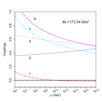
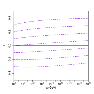
Figure 1: Running couplings with $m_{\rm top}=173.34{\rm GeV}$. Two-loop $\beta$ functions have been used for the standard model couplings.

The $\beta$ functions are effectively a set of differential equations which can be solved to obtain the dependence of the couplings on the renormalisation scale. This has been done in figure 1, using the flat-space two-loop $\beta$ functions for the couplings on the left hand plot Degrassi et al. (2012). Since the one-loop results work well enough for all of the couplings apart from $\lambda$, it is reasonable to use the one-loop result for $\beta_{\xi}$ which has been derived above. The running coupling $\xi(\mu)$, shown in the right-hand plot, displays very little change with energy, apart from a small increase of around $0.07$ from the Electroweak to the Planck scale.

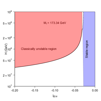
Figure 2: The inflationary Higgs instability region and the lower limit on $\xi_{EW}$ as a function of the Hubble parameter during inflation.

The running couplings can be combined with the field renormalisation to construct an improved form of the effective potential,

$$V_{\rm eff}=\frac{1}{2}\xi_{\rm eff}(\phi)R\,\phi^{2}+\frac{1}{4}\lambda_{\rm eff}(\phi)\,\phi^{4},$$ (12)

where the effective couplings combine the running coupling with the field renormalisation at $\mu=\phi$ . If $\lambda_{\rm eff}$ is negative at large $\phi$, then negative values for $\xi$ tend to destabilise the Higgs field during an early universe inflationary period. For some critical value $R_{c}$, the potential develops an inflection point and the field become classically unstable for $R>R_{c}$. The inflection point occurs when $V^{\prime}=V^{\prime\prime}=0$, which can be solved using the running couplings to obtain a relation between $R_{c}$ and the values of the couplings at the electroweak scale. Since most of the couplings are known, in effect we have a relation between $R_{c}$ and the value of the curvature coupling measured at the electroweak scale, $\xi_{EW}$. The region of instability for negative $\xi_{EW}$ is shown in figure 2, in terms of the Hubble parameter $H$, where $R=12H^{2}$. Curvature couplings $\xi_{EW}<-0.32$ can occur, but only in models of inflation which have unusually small values of the Hubble parameter.

Values of $\xi_{EW}>-0.32$ have the opposite effect and stabilise the Higgs field against decay associated with quantum tunnelling through the potential barrier. The probability of fluctuations through the potential barrier is exponentially suppressed with exponent $8\pi^{2}V(\phi_{c})/3H^{4}$ Espinosa et al. (2008). Figure 2 shows the parameter region for $8\pi^{2}V(\phi_{c})/3H^{4}>10$ and leads to the stability bound $\xi_{EW}>-0.3$. (Using a lower top quark mass $M_{t}=173\,{\rm GeV}$ raises the values of the Hubble parameter but leaves the limit on $\xi_{EW}$ unchanged.)

In summary, stability of the Higgs vacuum during early universe inflation sets limits on the curvature coupling. These limits have been shown to be frame-independent in the $|\xi|^{1/2}\phi\ll M_{p}$ limit, but only when quantum gravity effects are included and a covariant quantisation procedure such as Vilkovisky-DeWitt, is adopted. We finish with some brief remarks on on extending the renormalisation group calculations to the regime $|\xi|^{1/2}\phi\sim M_{p}$. This is technically feasible with the covariant approach, but moving to larger values of the Higgs field makes it necessary to consider the effects of higher order operators on the renormalisation group, and because of this predictability begins to be eroded Burgess et al. (2014). On the positive side, these higher border terms can stabilise the Higgs vacuum and remove the need for a separate field driving inflation.

References

- Degrassi et al. (2012) G. Degrassi, S. Di Vita, J. Elias-Miro, J. R. Espinosa, G. F. Giudice, et al., JHEP 1208, 098 (2012), arXiv:1205.6497 [hep-ph] .
- Espinosa et al. (2008) J. R. Espinosa, G. F. Giudice, and A. Riotto, JCAP 0805, 002 (2008), arXiv:0710.2484 [hep-ph] .
- De Simone et al. (2009) A. De Simone, M. P. Hertzberg, and F. Wilczek, Phys.Lett. B678, 1 (2009), arXiv:0812.4946 [hep-ph] .
- Barvinsky et al. (2012) A. Barvinsky, A. Y. Kamenshchik, C. Kiefer, A. Starobinsky, and C. Steinwachs, Eur.Phys.J. C72, 2219 (2012), arXiv:0910.1041 [hep-ph] .
- DeWitt (1965) B. S. DeWitt, Dynamical Theory of Groups and Fields (Gordon and Breach, 1965).
- Alvarez-Gaumé et al. (1981) L. Alvarez-Gaumé, D. Z. Freedman, and S. Mukhi, Annals of Physics 134, 85 (1981).
- Kamenshchik and Steinwachs (2015) A. Yu. Kamenshchik and C. F. Steinwachs, Phys. Rev. D91, 084033 (2015), arXiv:1408.5769 [gr-qc] .
- George et al. (2015) D. P. George, S. Mooij, and M. Postma, (2015), arXiv:1508.04660 [hep-th] .
- Herranen et al. (2014) M. Herranen, T. Markkanen, S. Nurmi, and A. Rajantie, Phys. Rev. Lett. 113, 211102 (2014), arXiv:1407.3141 [hep-ph] .
- Sher (1989) M. Sher, Phys. Rept. 179, 273 (1989).
- Vassilevich (2003) D. V. Vassilevich, Phys. Rept. 388, 279 (2003), arXiv:hep-th/0306138 [hep-th] .
- Vilkovisky (1984) G. A. Vilkovisky, in Quantum Theory of Gravity (Adam Hilger, 1984) p. 169.
- Barvinsky and Vilkovisky (1985) A. O. Barvinsky and G. A. Vilkovisky, Physics Reports 119, 1 (1985).
- Parker and Toms (2009) L. E. Parker and D. J. Toms, Quantum Field Theory in Curved Spacetime (Cambridge University Press, 2009).
- Barvinsky et al. (2009) A. Barvinsky, A. Y. Kamenshchik, C. Kiefer, A. Starobinsky, and C. Steinwachs, JCAP 0912, 003 (2009), arXiv:0904.1698 [hep-ph] .
- Note (1) In non-linear sigma model terms, the covariant metric expansion is .
- Moss (2014) I. G. Moss, (2014), arXiv:1409.2108 [hep-th] .
- Bezrukov and Shaposhnikov (2009) F. Bezrukov and M. Shaposhnikov, JHEP 07, 089 (2009), arXiv:0904.1537 [hep-ph] .
- Note (2) There is a proviso here that the effective mass terms must all be larger than the curvature.
- Burgess et al. (2014) C. P. Burgess, S. P. Patil, and M. Trott, JHEP 06, 010 (2014), arXiv:1402.1476 [hep-ph] .