A discontinuous Galerkin multiscale method for convection-diffusion problems

Abstract

We propose an discontinuous Galerkin local orthogonal decomposition multiscale method for convection-diffusion problems with rough, heterogeneous, and highly varying coefficients. The properties of the multiscale method and the discontinuous Galerkin method allows us to better cope with multiscale features as well as interior/boundary layers in the solution. In the proposed method the trail and test spaces are spanned by a corrected basis computed on localized patches of size $\mathcal{O}(H\log(H^{-1}))$, where $H$ is the mesh size. We prove convergence rates independent of the variation in the coefficients and present numerical experiments which verify the analytical findings.

1 Introduction

In this paper we consider numerical approximation of convection-diffusion problems with possible strong convection and with rough, heterogeneous, and highly varying coefficients, without assumption on scale separation or periodicity. This class of problems, normally refereed to as multiscale problem, are know to be very computational demanding and arise in many different areas of the engineering sciences, e.g., in porous media flow and composite materials. More precisely, we consider the following convection-diffusion equation: given any $f\in L^{2}(\Omega)$ we seek $u\in H^{1}_{0}(\Omega)=\{v\in H^{1}(\Omega)\mid v|_{\Gamma}=0\}$ such that

$$-\nabla\cdot A\nabla u+\mathbf{b}\cdot\nabla u =f\quad\text{in }\Omega,$$ (1)

is fulfilled in a weak sense, where $\Omega$ is the computational domain with boundary $\Gamma$. The multiscale coefficients $A,\mathbf{b}$ will be specified later. There are two key issues which make classical conforming finite element methods perform badly for these kind of problems,

• the multiscale features of the coefficient need to be resolved by the finite element mesh and

• strong convection leads to boundary and interior layers in the solution which need to be resolved.

To overcome the lack of performance using classical finite element methods in the case of multiscale features in the coefficient many different so called multiscale methods have been proposed, see [25, 26, 23, 7, 13, 12, 10, 11] among others, which perform localized fine scale computations to construct a different basis or a modified coarse scale operator. Common to the aforementioned approaches is that the performance of the method rely strongly on scale separation or periodicity of the diffusion coefficients. There is also approaches which perform well without scale separation or periodicity in the diffusion coefficient but to high computational cost by either having to solve eigenvalue problems [2] or where the support of the localized patches is large [37, 4]. See also [38].

In the variational multiscale method (VMS) framework [25, 26] the solution space is split into coarse and fine scale contribution. This idea was employed for multiscale problems in a adaptive setting for classical finite element in [31, 34, 32] and to the discontinuous Galerkin (DG) method in [14]. A further development is the local orthogonal decomposition (LOD) method, see [36, 20, 19] for classical finite element and [15] for DG methods. The LOD operates in linear complexity without any assumptions on scale separation or periodicity and the trail and test spaces are spanned by a corrected basis function computed on patches of size $\mathcal{O}(H\log(H^{-1}))$. The LOD has e.g. been applied to eigenvalue problems [35], non-linear elliptic problems [21], non-linear Schrödinger equation [17], and in Petrov-Galerkin formulation [16].

There is a vast literature on numerical methods for convection dominated problems, we reefer to [28, 24, 27], among others. There has also been a lot of work on DG methods, we refer to [39, 33, 3, 29] for some early work and to [8, 22, 40, 9] and references therein for recent development and a literature review. DG methods exhibit attractive properties for convection dominated problems, e.g., they have enhanced stability properties, good conservation property of the state variable, and the use of complex and/or irregular meshes are admissible. For multiscale methods for convection-diffusion problems, see e.g. [1, 41, 18].

In this paper we extended the analysis of the discontinuous Galerkin local orthogonal decomposition (DG-LOD) [15] to convection-diffusion problems. For problems with strong convection using the standard LOD won’t suffice, since convergence can no longer be guarantied. Instead we propose to include the convective term in the computations of the corrected basis functions. We prove convergence results under some assumptions of the magnitude of the convection and present a series of numerical experiment to verify the analytic findings. For problems with weak convection it is not necessary to include the convective part [21].

The outline of this paper is as follows. In section 2 the discrete setting and underlying DG method is presented. In section 3 the multiscale decomposition, the DG-LOD, and the corresponding convergence result are stated. In Section 4 numerical experiments are presented. Finally, the proofs for some of the theoretical results are given in Section 5.

2 Preliminaries

In this section we present some notations and properties frequently used in the paper.

2.1 Setting

Let $\Omega\subset\mathbb{R}^{d}$ for $d=2,3$ be a polygonal domain with Lipschitz boundary $\Gamma$. We assume that: the diffusion coefficients, $A\in L^{\infty}(\Omega,\mathbb{R}^{d\times d}_{sym})$, has uniform spectral bounds $0<\alpha,\beta<\infty$, defined by

$$0<\alpha:=\underset{x\in\Omega}{\operatorname{ess}\inf}\inf\limits_{v\in\mathbb{R}^{\operatorname*{d}}\setminus\{0\}}\dfrac{(A(x)v)\cdot v}{v\cdot v}\leq\underset{x\in\Omega}{\operatorname{ess}\sup}\sup\limits_{v\in\mathbb{R}^{\operatorname*{d}}\setminus\{0\}}\dfrac{(A(x)v)\cdot v}{v\cdot v}=:\beta<\infty,$$ (2)

and the convective coefficient, $\mathbf{b}\in[W_{\infty}^{1}(\Omega)]^{d}$, is divergence free

$$\nabla\cdot\mathbf{b}(x)=0\text{ a.e. }x\in\Omega.$$ (3)

We denote $C_{A}=(\beta/\alpha)^{1/2}$.

We will consider a coarse and a fine mesh, with mesh function $h$ and $H$ respectively. Furthermore, we assume that the fine mesh resolve and that the coarse mesh do not resolve the fine scale features in the coefficients. Let $\mathcal{T}_{k}$, for $k=\{h,H\}$, denote a shape-regular subdivision of $\Omega$ into (closed) regular simplexes or into quadrilaterals/hexahedras ($d=2/d=3$), given a mesh function $k:\mathcal{T}_{k}\to\mathbb{R}$ defined as $k:=\text{diam}(T)\in P_{0}(\mathcal{T}_{k})$ for all $T\in\mathcal{T}_{k}$. Also, let $\nabla_{k}v$ denote the $\mathcal{T}_{k}$-broken gradient defined as $(\nabla v)|_{T}=\nabla v|_{T}$ for all $T\in\mathcal{T}_{k}$. For simplicity we will also assume that $\mathcal{T}_{k}$ is conforming in the sense that no hanging nodes are allowed, but the analysis can easily be extend to non-conforming meshes with a finite number of hanging nodes on each edge. Let $\hat{T}$ be the reference simplex or (hyper)cube. We define $\mathcal{P}_{p}(\hat{T})$ to be the space of polynomials of degree less than or equal to $p$ if $\hat{T}$ is a simplex, or the space of polynomials of degree less than or equal to $p$, in each variable, if $\hat{T}$ is a (hyper)cube. The space of discontinuous piecewise polynomial function is defined by

$$P_{p}(\mathcal{T}_{k}):=\{v:\Omega\to\mathbb{R}\mid\forall T\in\mathcal{T}_{k},\,v|_{T}\circ F_{T}\in\mathcal{P}_{p}(\hat{T})\},$$ (4)

where $F_{T}:\hat{T}\to T$, $T\in\mathcal{T}_{k}$ is a family of element maps. We will work with the spaces $\mathcal{V}_{k}:=P_{1}(\mathcal{T}_{k})$. Let $\Pi_{p}(\mathcal{T}_{k}):L^{2}(\Omega)\to P_{p}(\mathcal{T}_{k})$ denote the $L^{2}$-projection onto $P_{p}(\mathcal{T}_{k})$. Also, let $\mathcal{E}_{k}$ denote the set of all edges in $\mathcal{T}_{k}$ where $\mathcal{E}_{k}(\Omega)$ and $\mathcal{E}_{k}(\Gamma)$ denote the set of interior and boundary edges, respectively. Given that $T^{+}$ and $T^{-}$ are two adjacent elements in $\mathcal{T}_{k}$ sharing an edge $e=T^{+}\cap T^{-}\in\mathcal{E}_{k}(\Omega)$, let $\nu_{e}$ be the the unit normal vector pointing from $T^{-}$ to $T^{+}$, and for $e\in\mathcal{E}_{k}(\Gamma)$ let $\nu_{e}$ be outward unit normal of $\Omega$. For any $v\in P_{p}(\mathcal{T}_{k})$ we denote the value on edge $e\in\mathcal{E}(\Omega)$ as $v^{\pm}=v|_{e\cap T^{\pm}}$. The jump and average of $v\in P_{p}(\mathcal{T}_{k})$ is defined as, $[v]=v^{-}-v^{+}$ and $\{v\}=(v^{-}+v^{+})/2$ respectively for $e\in\mathcal{E}_{k}(\Omega)$, and $[v]=\{v\}=v|_{e}$ for $e\in\mathcal{E}_{k}(\Gamma)$. For a real number $x$ we define its negative part as $x^{\ominus}=1/2(|x|-x)$.

Let $0\leq C<\infty$ denote any generic constant that neither depends on the mesh size or the variables $A$ and $\mathbf{b}$; then $a\lesssim b$ abbreviates the inequality $a\leq Cb$.

2.2 Discontinuous Galerkin discretization

For simplicity let the bilinear form $a_{h}(\cdot,\cdot):\mathcal{V}_{h}\times\mathcal{V}_{h}\to\mathbb{R}$, given any mesh function $h:\Omega\to P_{0}(\mathcal{T}_{h})$, be split into two parts

$$a_{h}(u,v):=a^{\operatorname*{d}}_{h}(u,v)+a^{\operatorname*{c}}_{h}(u,v),$$ (5)

where $a^{\operatorname*{d}}_{h}(\cdot,\cdot)$ represents the diffusion part and $a^{\operatorname*{c}}_{h}(\cdot,\cdot)$ represents the convection part. The diffusion part is approximated using a symmetric interior penalty method

$$a_{h}^{\operatorname*{d}}(u,v) :=(A\nabla_{h}u,\nabla_{h}v)_{L^{2}(\Omega)}+\sum_{e\in\mathcal{E}_{h}}\Big{(}\frac{\sigma_{e}}{h_{e}}([u],[v])_{L^{2}(e)}$$ (6)

$$\qquad-(\{\nu_{e}\cdot A\nabla u\},[v])_{L^{2}(e)}-(\{\nu_{e}\cdot A\nabla v\},[u]_{L^{2}(e)})\Big{)},$$

where $\sigma_{e}$ is a constant, depending on the diffusion, large enough to make $a_{h}^{\operatorname*{d}}(\cdot,\cdot)$ coercive. The convective part is approximated by

$$a_{h}^{\operatorname*{c}}(u,v):=(\mathbf{b}\cdot\nabla_{h}u,v)_{L^{2}(\Omega)}+\sum_{e\in\mathcal{E}_{h}(\Omega)}(b_{e}[u],[v])_{L^{2}(e)}$$ (7)

$$\qquad-\sum_{e\in\mathcal{E}_{h}(\Omega)}(\nu_{e}\cdot\mathbf{b}[u],\{v\})_{L^{2}(e)}+\sum_{e\in\mathcal{E}_{h}(\Gamma)}((\nu_{e}\cdot\mathbf{b})^{\ominus}u,v)_{L^{2}(e)},$$

where upwind is imposed choosing the stabilization term as $b_{e}=|\mathbf{b}\cdot\nu_{e}|/2$ [5].

The following definitions and results are needed both on the fine and coarse scale, for this sake let $k=\{h,H\}$. The energy norm on $\mathcal{V}_{k}$ is given by

$$|||v|||^{2}_{k,\operatorname*{d}} =\|A^{1/2}\nabla_{k}v\|^{2}_{L^{2}(\Omega)}+\sum_{e\in\mathcal{E}_{k}}\frac{\sigma_{e}}{k}\|[v]\|^{2}_{L^{2}(e)},$$ (8)

$$|||v|||^{2}_{k,\operatorname*{c}} =\sum_{e\in\mathcal{E}_{k}}\|b_{e}^{1/2}[v]\|^{2}_{L^{2}(e)},$$

$$|||v|||^{2}_{k} =|||v|||^{2}_{k,\operatorname*{d}}+|||v|||^{2}_{k,\operatorname*{c}}.$$

From Theorem 2.2 in [30] we have that for each $v\in\mathcal{V}_{k}$, there exist an averaging operator $\mathcal{I}^{c}_{k}:\mathcal{V}_{k}\to\mathcal{V}_{k}\cap H^{1}(\Omega)$ with the following property

$$\|\nabla_{k}(v-\mathcal{I}^{c}_{k}v)\|_{L^{2}(\Omega)}+\|k^{-1}(v-\mathcal{I}^{c}_{k}v)\|_{L^{2}(\Omega)}\lesssim\sum_{e\in\mathcal{E}_{k}}\frac{1}{k}\|[v]\|^{2}_{L^{2}(e)}.$$ (9)

In the error analysis we will also need a localized energy norm, defined in a domain $\omega\subset\Omega$ (aligned with the mesh $\mathcal{T}_{k}$) as

$$|||v|||^{2}_{k,\operatorname*{d},\omega} =\|A^{1/2}\nabla_{k}v\|^{2}_{L^{2}(\omega)}+\sum_{\begin{subarray}{c}e\in\mathcal{E}_{k}\\ e\cap\bar{\omega}\neq 0\end{subarray}}\frac{\sigma_{e}}{k}\|[v]\|^{2}_{L^{2}(e)},$$ (10)

$$|||v|||^{2}_{k,\operatorname*{c},\omega} =\sum_{\begin{subarray}{c}e\in\mathcal{E}_{k}\\ e\cap\bar{\omega}\neq 0\end{subarray}}\|b_{e}^{1/2}[v]\|^{2}_{L^{2}(e)},$$

$$|||v|||^{2}_{k,\omega} =|||v|||^{2}_{k,\operatorname*{d},\omega}+|||v|||^{2}_{k,\operatorname*{c},\omega}.$$

3 Multiscale method

In this section we preset the multiscale decomposition and extend the results in [15] to convection-diffusion problems. For the constants in the convergence results to be stable we assume the following relation of the convective term

$$\mathcal{O}\left(\frac{\|H\mathbf{b}\|_{L^{\infty}(\Omega)}}{\alpha}\right)\leq 1$$ (11)

How the magnitude of (11) affects the convergence of the method is investigated in the numerical experiments.

3.1 Multiscale decomposition

In order to do the multiscale decomposition the problem is divided into a coarse and a fine scale. To this end let $\mathcal{T}_{H}$ and $\mathcal{T}_{h}$, with the respective mesh function $H$ and $h$, denote the two different subdivisions, where $\mathcal{T}_{h}$ is constructed by some (possible adaptive) refinements of $\mathcal{T}_{H}$.

The aim of this section is to construct a coarse finite element space based on $\mathcal{T}_{H}$, which takes the fine scale behavior of the data into account. We assume that the mesh $\mathcal{T}_{h}$ resolves the variation in the data, i.e., the solution to: find $u_{h}\in\mathcal{V}_{h}$ such that

$$a_{h}(u_{h},v)=F(v)\quad\text{for all }v\in\mathcal{V}_{h},$$ (12)

gives a sufficiently good approximation of the weak solution $u$ to (1). Note however that $u_{h}$ never have to be computed in practice, it only acts as a reference solution. We introduce a coarse projection operator $\Pi_{H}:=\Pi_{1}(\mathcal{T}_{H})$ and let the fine scale reminder space be defined by the kernel of $\Pi_{H}$, i.e.,

$$\mathcal{V}^{\operatorname*{f}}:=\{v\in\mathcal{V}_{h}\mid\Pi_{H}v=0\}\subset\mathcal{V}_{h}.$$ (13)

The coarse projection operator has the following approximation and stability properties.

Lemma 1.

For any $v\in\mathcal{V}_{h}$ and $T\in\mathcal{T}_{H}$, the approximation property

$$H|_{T}^{-1}\|v-\Pi_{H}v\|_{L^{2}(T)}\lesssim\alpha^{-1/2}|||v|||_{h,T},$$ (14)

and stability estimate

$$|||\Pi_{H}v|||_{H}\lesssim C_{s}|||v|||_{\operatorname*{h}},$$ (15)

is satisfied, with

$$C_{s}=\left(C_{A}^{2}+\frac{\|H\mathbf{b}\|_{L^{\infty}(\Omega)}}{\alpha}\right)^{1/2}.$$ (16)

Proof.

The approximation property follows directly from [15, Lemma 5]. Let $\mathcal{C}_{H}:H^{1}\to H^{1}\cap\mathcal{V}_{H}$ be a Clément type interpolation operator proposed in [6, Section 6] which satisfy

$$\|\nabla\mathcal{C}_{H}u\|_{L^{2}(T)}+\|H^{-1}(u-\mathcal{C}_{H}u)\|_{L^{2}(T)}\lesssim\|\nabla u\|_{L^{2}(\omega_{T}^{1})},$$ (17)

where $\omega_{T}^{1}=\text{int}(\cup\{T^{\prime}\in T_{H}\mid T\cap T\neq 0\})$ are the union of all elements that share a edge with $T$. We define the conforming function $v_{c}=\mathcal{C}_{H}\mathcal{I}^{c}_{h}v$ using averaging operator in (9). We obtain

$$|||\Pi_{H}v|||_{H}^{2}=\sum_{T\in\mathcal{T}_{H}}\|A^{1/2}\nabla(\Pi_{H}v-\Pi_{0}v)\|^{2}_{L^{2}(T)}$$ (18)

$$\qquad+\sum_{e\in\mathcal{E}_{h}(\Omega\cup\Gamma_{D})}\Big{(}\frac{\sigma}{H}\|[v_{c}-\Pi_{H}v]\|^{2}_{L^{2}(e)}+\|b_{e}^{1/2}[v_{c}-\Pi_{H}v]\|^{2}\Big{)}$$

$$\lesssim\sum_{T\in\mathcal{T}_{H}}\beta\left(\frac{1}{H^{2}}\|v-\Pi_{0}v\|^{2}_{L^{2}(T)}+\left(\frac{1}{H^{2}}+\frac{\|\mathbf{b}\|_{L^{\infty}(T)}}{H}\right)\|v_{c}-v\|^{2}_{L^{2}(T)}\right)$$

using that $\Pi_{0}:=\Pi_{0}(\mathcal{T}_{H})$ is the $L^{2}$-projection onto constants, a trace inequality, and stability of $\Pi_{H}$. Next, using that

$$\|\mathcal{C}_{H}\mathcal{I}^{c}_{h}v-v\|_{L^{2}(\Omega)} \leq\|\mathcal{C}_{H}\mathcal{I}^{c}_{h}v-\mathcal{I}^{c}_{h}v\|_{L^{2}(\Omega)}+\|\mathcal{I}^{c}_{h}v-v\|_{L^{2}(\Omega)}$$ (19)

$$\lesssim H\|\nabla\mathcal{I}^{c}_{h}v\|_{L^{2}(\Omega)}+\|\mathcal{I}^{c}_{h}v-v\|_{L^{2}(\Omega)}$$

$$\lesssim\alpha^{-1/2}H|||v|||_{\operatorname*{h}}$$

in (18) concludes the proof. ∎

The following lemma shows that for every $v_{H}\in\mathcal{V}_{H}$ there exist a (non-unique) $v\in\Pi_{H}^{-1}v_{H}\in\mathcal{V}_{h}$ in the preimage of $\Pi_{H}$ which is $H^{1}(\Omega)$ conforming.

Lemma 2.

For each $v_{H}\in\mathcal{V}_{H}$, there exist a $v\in\mathcal{V}_{h}\cap H^{1}(\Omega)$ such that $\Pi_{H}v=v_{H}$, $|||v|||_{\operatorname*{h}}\lesssim C_{A}|||v_{H}|||_{H}$, and $\operatorname*{supp}(v)\subset\operatorname*{supp}(\mathcal{I}^{\operatorname*{c}}_{H}v_{H})$.

Proof.

Follows directly from [15, Lemma 6], since $v\in H^{1}(\Omega)$. ∎

The next step is to split any $v\in\mathcal{V}_{h}$ into some coarse part based on $\mathcal{T}_{H}$, such that the fine scale reminder in the space $\mathcal{V}^{\operatorname*{f}}$ is sufficiently small. A naive way to do this splitting is to use a $L^{2}$-orthogonal split. An alternative definition of the coarse space is $\mathcal{V}_{H}=\Pi_{H}\mathcal{V}_{h}$. A set of basis functions that span $\mathcal{V}_{H}$ is the element-wise Lagrange basis functions $\{\lambda_{T,j}\mid T\in\mathcal{T}_{H},\,j=1,\dots,r\}$ where $r=(1+d)$ for simplexes or $r=2^{d}$ for quadrilaterals/hexahedra. The space $\mathcal{V}_{H}$ is known to give poor approximation properties if $\mathcal{T}_{H}$ does not resolve the variable coefficients in (1). We will use another choice, see [36, 15], based on $a_{h}(\cdot,\cdot)$, to construct a space of corrected basis functions. To this end, we define a fine scale projection operator $\mathfrak{F}:\mathcal{V}_{h}\to\mathcal{V}^{\operatorname*{f}}$ by

$$a_{h}(\mathfrak{F}v,w)=a_{h}(v,w)\quad\text{for all }w\in\mathcal{V}^{\operatorname*{f}},$$ (20)

and let the corrected coarse space be defined as

$$\mathcal{V}^{ms}_{H}:=(1-\mathfrak{F})\mathcal{V}_{H}.$$ (21)

The corrected space are spanned by corrected basis functions $\mathcal{V}^{ms}_{H}:=\{\lambda_{T,j}-\phi_{T,j}\mid T\in\mathcal{T}_{H},\,j=1,\dots,r\}$ which can be computed as: for all $T\in\mathcal{T}_{H},\,j=1,\dots,r$ find $\phi_{T,j}\in\mathcal{V}^{\operatorname*{f}}$ such that

$$a_{h}(\phi_{T,j},v)=a_{h}(\lambda_{T,j},v)\quad\text{for all }v\in\mathcal{V}^{\operatorname*{f}}.$$ (22)

Note that, $\text{dim}(\mathcal{V}^{ms}_{H})=\text{dim}(\mathcal{V}_{H})$. From (21) we have that any $v_{h}\in\mathcal{V}_{h}$ can be decomposed into a coarse $v^{ms}_{H}\in\mathcal{V}^{ms}_{H}$ and a fine $v^{f}\in\mathcal{V}^{\operatorname*{f}}$ scale contribution, $v_{h}=v^{ms}_{H}+v^{f}$.

Lemma 3 (Stability of the corrected basis function).

For all $T\in\mathcal{T}_{H},\,j=1,\dots,r$, the following estimate

$$|||\phi_{T,h}-\lambda_{T,j}|||_{\operatorname*{h}}\lesssim C_{\phi}\beta^{1/2}\|H^{-1}\lambda_{T,j}\|_{L^{2}(\Omega)}$$ (23)

holds, where $C_{\phi}=(C_{A}^{2}+\|H\mathbf{b}\|_{L^{\infty}(\Omega)}\alpha^{-1})^{1/2}$.

Proof.

Let $v=\lambda_{T,j}-b_{T,j}\in\mathcal{V}^{\operatorname*{f}}$, where $b_{T,j}\in H^{1}_{0}(T)$, $\Pi_{H}b_{T,j}=\lambda_{T,j}$, $|||b_{T,j}|||_{\operatorname*{h}}\leq C_{A}|||\lambda_{T,j}|||_{H}$ from Lemma 2. We have

$$|||\phi_{T,h}-\lambda_{T,j}|||_{\operatorname*{h}}^{2}\lesssim a_{h}(\phi_{T,h}-\lambda_{T,j},\phi_{T,h}-\lambda_{T,j})$$ (24)

$$=a_{h}(\phi_{T,h}-\lambda_{T,j},v-\lambda_{T,j})=a_{h}(\phi_{T,h}-\lambda_{T,j},b_{T,j})$$

$$=a_{h}^{d}(\phi_{T,h}-\lambda_{T,j},b_{T,j})+\left(\mathbf{b}\cdot\nabla_{h}(\phi_{T,h}-\lambda_{T,j}),b_{T,j}\right)_{L^{2}(\Omega)}.$$

Using that the diffusion part in (24) of the bilinear form is continuous in $(\mathcal{V}_{h}\times\mathcal{V}_{h})$ with the constant $C_{A}$, Lemma 2, and a inverse inequality, we get

$$a_{h}^{d}(\phi_{T,h}-\lambda_{T,j},b_{T,j}) \lesssim C_{A}|||\phi_{T,h}-\lambda_{T,j}|||_{\operatorname*{h}}|||b_{T,j}|||_{\operatorname*{h}}$$ (25)

$$\lesssim C_{A}^{2}|||\phi_{T,h}-\lambda_{T,j}|||_{\operatorname*{h}}|||\lambda_{T,j}|||_{H}$$

$$\lesssim C_{A}^{2}\beta^{1/2}|||\phi_{T,h}-\lambda_{T,j}|||_{\operatorname*{h}}\|H^{-1}\lambda_{T,j}\|_{L^{2}(T)}.$$

For the convection part in (24), we have

$$(\mathbf{b}\cdot\nabla_{h}(\phi_{T,h}-\lambda_{T,j}),b_{T,j})_{L^{2}(\Omega)}$$ (26)

$$\lesssim\|H\mathbf{b}\cdot\nabla_{h}(\phi_{T,h}-\lambda_{T,j})\|_{L^{2}(\Omega)}\|H^{-1}b_{T,j}\|_{L^{2}(\Omega)}$$

$$\lesssim\|H\mathbf{b}\|_{L^{\infty}(\Omega)}\|\nabla_{h}(\phi_{T,h}-\lambda_{T,j})\|_{L^{2}(\Omega)}\|H^{-1}\lambda_{T,j}\|_{L^{2}(\Omega)},$$

and obtain

$$|||\phi_{T,h}-\lambda_{T,j}|||_{\operatorname*{h}}\leq C_{\phi}\beta^{1/2}\|H^{-1}\lambda_{T,j}\|_{L^{2}(\Omega)}.$$ (27)

with $C_{\phi}=(C_{A}^{2}+\|H\mathbf{b}\|_{L^{\infty}(\Omega)}\alpha^{-1})^{1/2}$. ∎

3.2 Ideal discontinuous Galerkin multiscale method

An ideal multiscale method seeks $u^{ms}_{H}\in\mathcal{V}^{ms}_{H}$ such that

$$a_{h}(u^{ms}_{H},v)=F(v)\quad\text{for all }v\in\mathcal{V}^{ms}_{H}.$$ (28)

Note that, to construct in the space $\mathcal{V}^{ms}_{H}$ a variational problem has to be solved on the whole domain $\Omega$ for each basis function, which is not feasible for real computations. The following theorem shows the convergence of the ideal (non-realistic) multiscale method.

Theorem 4.

Let $u_{h}\in\mathcal{V}_{h}$ be the solution to (12), and $u^{ms}_{H}\in\mathcal{V}^{ms}_{H}$ be the solution to (28), then

$$|||u_{h}-u^{ms}_{H}|||\lesssim C_{1}\alpha^{-1/2}||H(f-\Pi_{H}f)||_{L^{2}(\Omega)}$$ (29)

holds, with $C_{1}=C_{A}+\|H\mathbf{b}\|_{L^{\infty}(\Omega)}\alpha^{-1}$

Proof.

See Section 5. ∎

3.3 Discontinuous Galerkin multiscale method

The fast decay of the corrected basis functions (Lemma 6), motivates us to solve the corrector functions on localized patches. This introduces a localization error, but choosing the patch size as $\mathcal{O}(H\log(H^{-1}))$ (Theorem 7) the localization error has the same convergence rate as the ideal multiscale method in Theorem 4. The corrector functions are solved on element patches, defined as follows.

Definition 5.

For all $T\in\mathcal{T}_{H}$, let $\omega^{L}_{T}$ be a patch centered around element $T$ with size $L$, defined as

$$\omega^{0}_{T} :=\mathrm{int}(T),$$ (30)

$$\omega^{L}_{T} :=\mathrm{int}(\cup\{T^{\prime}\in T_{H}\mid T\cap\bar{\omega}^{L-1}_{T}\neq 0\}),\quad L=1,2,\dots.$$

See Figure 1 for an illustration.

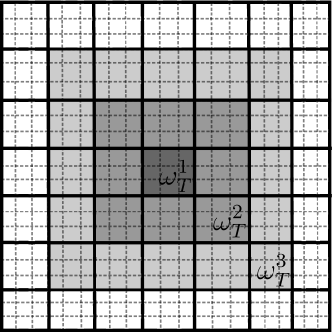
Figure 1: Example of a patch with one layer, $\omega^{1}_{T}$, two layers $\omega^{2}_{T}$, and three layers $\omega^{3}_{T}$, centered around element T.

The localized corrector functions are calculated as follows: for all $\{T\in\mathcal{T}_{H},j=1,\dots,r\}$ find $\phi^{L}_{T,j}\in\mathcal{V}^{f}(\omega^{L}_{T})=\{v\in\mathcal{V}^{\operatorname*{f}}\mid v|_{\Omega\setminus\omega^{L}_{T}}=0\}$ such that

$$a_{h}(\phi^{L}_{T,j},v)=a_{h}(\lambda_{T,j},v),\quad\text{for all }v\in\mathcal{V}^{f}(\omega^{L}_{T}).$$ (31)

The decay of the corrected basis function is given in the following lemma.

Lemma 6.

For all $T\in\mathcal{T}_{H}$, $j=1,\dots,r$ where $\phi_{T,j}$ is the solution to (22) and $\phi^{L}_{T,j}$ is the solution to (36), the following estimate

$$\left|\left|\left|\phi_{T,j}-\phi^{L}_{T,j}\right|\right|\right|_{h}\lesssim C_{2}\gamma^{L}|||\lambda_{T,j}-\phi^{L}_{T,j}|||_{\operatorname*{h}}$$ (32)

holds, where $L=\ell k$ is the size of the patch, $0<\gamma=(\ell^{-1}C_{3})^{\frac{\ell(k-1)-1}{2\ell k(\ell+1)}}<1$, $C_{2}=C_{c}C_{\zeta}(1+C_{A}C_{s})$, and $C_{3}=C(C_{A}^{2}+\|H\mathbf{b}\|_{L^{\infty}(\Omega)}\alpha^{-1})$, where $C$ is a generic constants neither depending on the mesh size, the size of the patches, or the problem data.

Proof.

See Section 5. ∎

The space of localized corrected basis function is defined by $\mathcal{V}^{ms,L}_{H}:=\{\phi^{L}_{T,j}-\lambda_{T,j}\mid T\in\mathcal{T}_{H},\,r=1,\dots,r\}$. The DG multiscale method reads: find $u^{ms,L}_{H}\in\mathcal{V}^{ms,L}_{H}$ such that

$$a_{h}(u^{ms,L}_{H},v)=F(v)\quad\text{for all }v\in\mathcal{V}^{ms,L}_{H}.$$ (33)

An error bound for the DG multiscale method using a localized corrected basis is given in Theorem 7. Note that it is only the first term $|||u-u_{h}|||_{\operatorname*{h}}$ in Theorem 7 that depends on the regularity of $u$.

Theorem 7.

Let $u_{h}\in\mathcal{V}_{h}$ and $u^{ms,L}_{H}\in\mathcal{V}^{ms,L}_{H}$ be the solutions to (12) and (33), respectively. Then

$$|||u-u^{ms,L}_{H}|||_{\operatorname*{h}}\leq |||u-u_{h}|||_{\operatorname*{h}}+C_{c}\alpha^{-1/2}\|H(f-\Pi_{H}f)\|_{L^{2}(\Omega)}$$ (34)

$$+C_{5}\|H^{-1}\|_{L^{\infty}(\Omega)}L^{d/2}\gamma^{L}\|f\|_{L^{2}(\Omega)}$$

holds, where $L$ is the size of the patches, $C_{1}$ is a constant defined in Theorem 4, $0<\gamma<1$ and $C_{5}=C_{4}^{1/2}C_{2}C_{\phi}C_{A}$, where $C_{4}=C_{c}^{2}C_{\zeta}^{2}(1+C_{A}C_{s})^{2}$ is defined in Lemma 13, and $C_{2}$ and $\gamma$ are defined in Lemma 6.

Proof.

See Section 5. ∎

Remark 8.

Theorem 7 is simplified to,

$$|||u-u^{ms,L}_{H}|||_{\operatorname*{h}}\leq|||u-u_{h}|||_{\operatorname*{h}}+C_{1}\|H\|_{L^{\infty}(\Omega)}.$$ (35)

given that the patch size is chosen as $L=\lceil C\log(H^{-1})\rceil$ with an appropriate $C$ and $\|f\|_{L^{2}}=1$. In the numerical experiments we choose $C=2$.

Remark 9.

If the convective term is small it is not necessary to include it in the computation of the correctors [21]. Instead the following correctors can be used: for all $\{T\in\mathcal{T}_{H},j=1,\dots,r\}$ find $\hat{\phi}^{L}_{T,j}\in\mathcal{V}^{f}(\omega^{L}_{T})$ such that

$$a_{h}^{\mathrm{d}}(\hat{\phi}^{L}_{T,j},v)=a_{h}^{\mathrm{d}}(\lambda_{T,j},v),\quad\text{for all }v\in\mathcal{V}^{f}(\omega^{L}_{T}).$$ (36)

This gives the right convergence results if

$$\mathcal{O}\left(\frac{\|\mathbf{b}\|_{L^{\infty}(\Omega)}}{\alpha}\right)=1$$ (37)

compared to (11) if the convective term is included.

4 Numerical experiment

We consider the domain $\Omega=[0,1]\times[0,1]$ and the forcing function $f=1+\cos(2\pi x)\cos(2\pi y)$. The localization parameter which determine the size of the patches is chosen as $L=\lceil 2\log(H^{-1})\rceil$, i.e., the size of the patches are $2H\log(H^{-1})$. Consider a coarse quadrilateral mesh, $\mathcal{T}_{H}$, of size $H=2^{-i}$, $i=2,3,4,5$. The corrector functions are solved on sub-grids of the quadrilateral mesh, $\mathcal{T}_{h}$, where $h=2^{-7}$. We consider three different permeabilities: $A_{1}=1$, $A_{2}=A_{2}(y)$ which is piecewise constant with respect to a Cartesian grid of width $2^{-6}$ in y-direction taking the values $1$ or $0.01$, and $A_{3}=A_{3}(x,y)$ which is piecewise constant with respect to a Cartesian grid of width $2^{-6}$ both in the x- and y-directions, bounded below by $\alpha=0.05$ and has a maximum ratio $\beta/\alpha=4\cdot 10^{5}$. The permeability $A_{3}$ is taken from the $31$ layer in the SPE 10 benchmark problem, see http:www.spe.org/web/csp/. The diffusion coefficients $A_{2}$ and $A_{3}$ are illustrated in Figure 2.

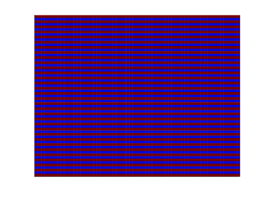
(a) $A_{2}$

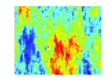
(b) $A_{3}$

Figure 2: The diffusion coefficients $A_{2}$ and $A_{3}$ in log scale.

For the convection term we consider: $\mathbf{b}=[C,0]$, for different values of $C$.

To investigate how the error in relative energy-norm, $|||u_{h}-u^{ms,L}_{H}|||/|||u_{h}|||$, depends on the magnitude of the convection we consider: $A_{1}$ and $\mathbf{b}=[C,0]$ with $C=\{32,64,128\}$. Figure 3 shows the convergence in energy-norm as a function of the coarse mesh size $H$ for the different values of $C$.

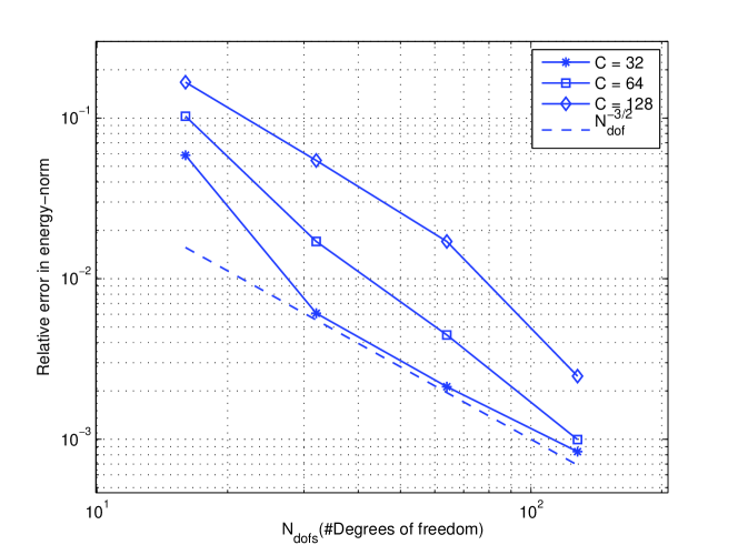
Figure 3: The number degrees of freedom ($N_{dof}$) vs. the relative error in energy-norm, for different sizes of the convection term, $C$.

Also, to see the effect of heterogeneous diffusion of the error in the relative energy-norm, $|||u_{h}-u^{ms,L}_{H}|||/|||u_{h}|||$, we consider: Figure 4 which shows the error in relative energy-norm using $A_{2}$ and $\mathbf{b}=[1,0]$ and Figure 5 which shows the error in relative energy-norm using $A_{3}$ and $\mathbf{b}=[512,0]$.

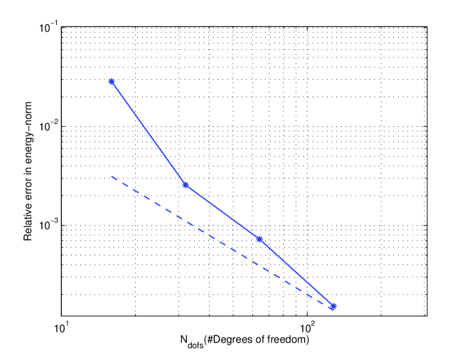
Figure 4: The number degrees of freedom ($N_{dof}$) vs. the relative error in energy-norm, using a high contrast diffusion coefficients $A_{2}$ and $\mathbf{b}=[1,0]$. The dotted line corresponds to $N_{dof}^{-3/2}$.

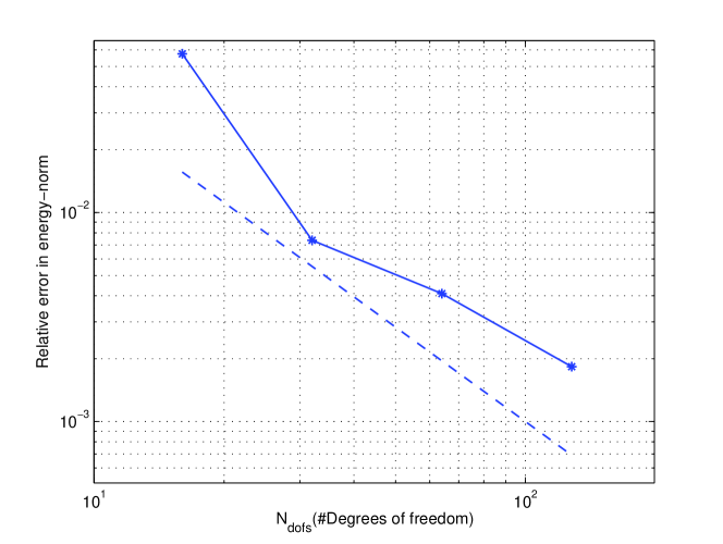
Figure 5: The number degrees of freedom ($N_{dof}$) vs. the relative error in energy-norm, using a high contrast diffusion coefficients $A_{3}$ and $\mathbf{b}=[512,0]$. The dotted line corresponds to $N_{dof}^{-3/2}$.

We obtain $H^{3}$ convergence of the DG multiscale method to a reference solution in the relative energy-norm, $|||u_{h}-u^{ms,L}_{H}|||/|||u_{h}|||$, independent of the variation in the coefficients or regularity of the underlying solution.

5 Proofs from Section 3

In this section we state the proofs of the main results which was postponed from in section 3. To this end we start by proving some technical lemmas in Section 5.1 which we use to prove the main results in Section 5.2.

5.1 Technical lemmas

In the proofs of the main results, Theorem 4, Lemma 6, and Theorem 7, we will need some definitions and technical lemmas stated below.

Continuity of the DG bilinear form for convective problems can be proven on a orthogonal subset of $\mathcal{V}_{h}$. The space $\mathcal{V}^{\operatorname*{f}}$ is an orthogonal subset of $\mathcal{V}_{h}$ but on a coarse scale.

Lemma 10 (Continuity in $(\mathcal{V}_{h}\times\mathcal{V}^{\operatorname*{f}})$ and $(\mathcal{V}^{\operatorname*{f}}\times\mathcal{V}_{h})$).

For all, $(u,v)\in\mathcal{V}^{\operatorname*{f}}\times\mathcal{V}_{h}$ or in $\mathcal{V}_{h}\times\mathcal{V}^{\operatorname*{f}}$ , it holds

$$a(v,w)\lesssim C_{c}|||v|||_{\operatorname*{h}}|||w|||_{\operatorname*{h}}$$ (38)

where

$$C_{c}=C_{A}+\|H\mathbf{b}\|_{L^{\infty}(\Omega)}\alpha^{-1}.$$ (39)

Proof.

Since $a^{d}_{h}$ is continuous in $(\mathcal{V}_{h}\times\mathcal{V}_{h})$ with the constant $C_{A}$, continuity in $(\mathcal{V}^{\operatorname*{f}}\times\mathcal{V}_{h})$ follows from $\mathcal{V}^{\operatorname*{f}}\subset\mathcal{V}_{h}$. For the convective part $a^{\operatorname*{c}}_{h}$, we have

$$a^{\operatorname*{c}}(v,w) =\sum_{T\in\mathcal{T}_{h}}(\mathbf{b}\cdot\nabla v,w)_{L^{2}(T)}+\sum_{e\in\mathcal{E}_{k}}(b_{e}[v],[w])_{L^{2}(e)}$$ (40)

$$\qquad-\sum_{e\in\mathcal{E}_{k}(\Omega)}(\nu_{e}\cdot\mathbf{b}[v],\{w\})_{L^{2}(e)}+\sum_{e\in\mathcal{E}_{k}(\Gamma)}((\nu_{e}\cdot\mathbf{b})^{\ominus}v,w)_{L^{2}(e)}$$

$$\lesssim\sum_{T\in\mathcal{T}_{h}}\left(\|\mathbf{b}\|_{L^{\infty}(T)}\|\nabla v\|_{L^{2}(T)}\|w-\Pi_{H}w\|_{L^{2}(T)}\right)$$

$$\qquad+\sum_{e\in\mathcal{E}_{k}}\Big{(}\|\mathbf{b}\|_{L^{\infty}(e)}h^{-1/2}\|[v]\|_{L^{2}(e)}\|w\|_{L^{2}(S^{+}\cup S^{-})}\Big{)}.$$

where $S^{+},S^{-}\in\mathcal{T}_{h}$ and $e=S^{+}\cap S^{-}$. Using a discrete Cauchy-Schwartz inequality and summing over the coarse elements, we get

$$a^{\operatorname*{c}}(v,w) \lesssim\alpha^{-1/2}\|H\mathbf{b}\|_{L^{\infty}(\Omega)}|||v|||_{\operatorname*{h}}\|H^{-1}(w-\Pi_{H}w)\|_{L^{2}(\Omega)},$$ (41)

$$\lesssim\|H\mathbf{b}\|_{L^{\infty}(\Omega)}\alpha^{-1}|||v|||_{\operatorname*{h}}|||w|||_{\operatorname*{h}},$$

which concludes the proof for $(\mathcal{V}_{h}\times\mathcal{V}^{\operatorname*{f}})$. The proof of $(\mathcal{V}^{\operatorname*{f}}\times\mathcal{V}_{h})$ is obtained by first integrating $(\mathbf{b}\cdot\nabla u,v)_{L^{2}(T)}$ by parts. ∎

The following cut-off function will be frequently used in the proof of the main results.

Definition 11.

The function $\zeta^{d,D}\in P_{o}(\mathcal{T}_{h})$, for $D>d$, is a cut off function fulfilling the following condition

$$\zeta^{d,D}_{T}|_{\omega^{d}_{T}} =1,$$ (42)

$$\zeta^{d,D}_{T}|_{\Omega\setminus\omega^{D}_{T}} =0,$$

$$\|[\zeta^{d,D}_{T}]\|_{L^{\infty}(\mathcal{E}_{h}(T))} \lesssim\frac{\|h\|_{L^{\infty}(T)}}{(D-d)H|_{T}},$$

and $||[\zeta^{d,D}]||_{L^{\infty}(\partial(\omega^{D}_{T}\setminus\omega^{d}_{T}))}=0$, for all $T\in\mathcal{T}_{H}$.

For the cut off function has the following stability property.

Lemma 12.

For any $v\in\mathcal{V}_{h}$ and $\zeta^{d,D}_{T}$ from Definition 11, the estimate,

$$|||\zeta^{d,D}_{T}v|||_{\operatorname*{h}}\lesssim C_{\zeta}|||v|||_{h,\omega^{D}_{T}},$$ (43)

holds, where $C_{\zeta}=(C_{A}^{2}+\|h\mathbf{b}\|_{L^{\infty}(\Omega)}/\alpha)^{1/2}$.

Proof.

For the diffusion part we use the following result from [15],

$$|||(1-\zeta^{d,D}_{T})v|||_{\operatorname*{h},\operatorname*{d}}\lesssim C_{A}|||v|||_{h,\Omega\setminus\omega_{T}^{L-1}}$$ (44)

and focus on the convective part. We obtain

$$|||(1-\zeta^{d,D}_{T})v|||_{\operatorname*{h},\operatorname*{c}}^{2}$$ (45)

$$=\sum_{e\in\mathcal{E}_{h}}\|b_{e}^{1/2}[(1-\zeta^{d,D}_{T})v]\|^{2}_{L^{2}(e)}$$

$$\leq\sum_{\begin{subarray}{c}e\in\mathcal{E}_{h}:\\ e\cap\omega^{L-1}_{T}\neq 0\end{subarray}}\left(\|b_{e}^{1/2}[v]\|^{2}_{L^{2}(e)}+\|h\|_{L^{\infty}(S^{+}\cup S^{-})}^{2}\|H^{-1}b_{e}^{1/2}\{v\}\|^{2}_{L^{2}(e)}\right)$$

$$\lesssim\sum_{\begin{subarray}{c}T\in\mathcal{T}_{H}:\\ e\cap\omega^{L-1}_{T}\neq 0\end{subarray}}\|h\mathbf{b}\|_{L^{\infty}(T)}\left(\|h^{-1/2}[v]\|^{2}_{L^{2}(e)}+\|H^{-1}(v-\Pi_{H}v)\|^{2}_{L^{2}(T)}\right)$$

$$\lesssim\frac{\|h\mathbf{b}\|_{L^{\infty}(\Omega)}}{\alpha}|||v|||_{h,\Omega\setminus\omega^{L-1}}^{2},$$

using $[vw]=\{v\}[w]+\{w\}[v]$, the triangle inequality, and a trace inequality. The proof is concluded using (44) and (45). ∎

The following lemmas will be necessary in order to prove Theorem 7.

Lemma 13.

The following estimate,

$$|||\sum_{T\in\mathcal{T}_{H},\,j=1,\dots,r}v_{j}(\phi_{T,j}-\phi^{L}_{T,j})|||_{\operatorname*{h}}^{2}\lesssim C_{4}L^{d}\sum_{T\in\mathcal{T}_{H},\,j=1,\dots,r}|v_{j}|^{2}|||\phi_{T,j}-\phi^{L}_{T,j}|||_{\operatorname*{h}}^{2},$$ (46)

holds, where $C_{4}=C_{c}^{2}C_{\zeta}^{2}(1+C_{A}C_{s})^{2}$.

Proof.

The proof is analogous with the proof of Lemma 12 in [15]. ∎

5.2 Proof of main results

We are now ready to prove, Theorem 4, Lemma 6, and Theorem 7.

Theorem 4.

Let us decompose $u_{h}$ into a coarse contribution, $v^{ms}_{H}\in\mathcal{V}^{ms}_{H}$, and a fine scale remainder, $v^{f}\in\mathcal{V}^{\operatorname*{f}}$, i.e., $u_{h}=v^{ms}_{H}+v^{f}$. For $v^{f}$ we have

$$|||v^{f}|||_{\operatorname*{h}}^{2} \lesssim a_{h}(v^{f},v^{f})=a_{h}(u_{h},v^{f})=(f,v^{f})_{L^{2}(\Omega)}$$ (47)

$$=(f-\Pi_{H}f,v^{f}-\Pi_{H}v^{f})_{L^{2}(\Omega)}$$

$$\leq\|H(f-\Pi_{H}f)\|_{L^{2}(\Omega)}\|H^{-1}(v^{f}-\Pi_{H}v^{f})||_{L^{2}(\Omega)}$$

$$\leq\alpha^{-1/2}\|H(f-\Pi_{H}f)\|_{L^{2}(\Omega)}|||v^{f}|||_{\operatorname*{h}}.$$

Using continuity, we get

$$|||u_{h}-u^{ms}_{H}|||_{\operatorname*{h}}^{2} \lesssim a_{h}(u_{h}-u^{ms}_{H},u_{h}-u^{ms}_{H})=a_{h}(u_{h}-u^{ms}_{H},u_{h}-v^{ms}_{H})$$ (48)

$$\lesssim C_{c}|||u_{h}-u^{ms}_{H}|||_{\operatorname*{h}}|||u_{h}-v^{ms}_{H}|||_{\operatorname*{h}},$$

which concludes the proof together with (47). ∎

Lemma 6.

Define $e:=\phi_{T,j}-\phi_{T,j}^{L}$ where $\phi_{T,j}\in\mathcal{V}^{\operatorname*{f}}$ and $\phi_{T,j}^{L}\in\mathcal{V}^{f}(\omega^{L}_{T})$. We have

$$\left|\left|\left|e\right|\right|\right|^{2}_{h}\lesssim a_{h}(e,\phi_{T,j}-\phi_{T,j}^{L})=a_{h}(e,\phi_{T,j}-v)\lesssim C_{c}|||e|||_{\operatorname*{h}}|||\phi_{T,j}-v|||_{\operatorname*{h}}.$$ (49)

Furthermore from Lemma 2, there exist a $v=\zeta^{L-1,L}_{T}\phi_{T,j}-b_{T}\in\mathcal{V}^{f}(\omega^{L}_{T})$ such that $\Pi_{H}b_{T}=\Pi_{H}(\zeta^{L-1,L}_{T}\phi_{T,j})$ and $|||b_{T}|||_{\operatorname*{h}}\lesssim C_{A}|||\Pi_{H}(\zeta^{L-1,L}_{T}\phi_{T,j})|||_{H}$, we have

$$\left|\left|\left|e\right|\right|\right|_{h}\lesssim C_{c}\left(|||(1-\zeta^{L-1,L}_{T})\phi_{T,j}|||_{\operatorname*{h}}+|||b_{T}|||_{\operatorname*{h}}\right),$$ (50)

where

$$|||b_{T}|||_{\operatorname*{h}} \lesssim C_{A}|||\Pi_{H}\zeta^{L-1,L}_{T}\phi_{T,j}|||_{H}=C_{A}|||\Pi_{H}(1-\zeta^{L-1,L}_{T})\phi_{T,j}|||_{H}$$ (51)

$$\lesssim C_{A}C_{s}|||(1-\zeta^{L-1,L}_{T})\phi_{T,j}|||_{\operatorname*{h}}\lesssim C_{A}C_{s}C_{\zeta}|||\phi_{T,j}|||_{h,\Omega\setminus\omega^{L-1}_{T}}.$$

using Lemma 2, Lemma 1, and Lemma 12. We obtain,

$$\left|\left|\left|e\right|\right|\right|_{h}\lesssim C_{2}|||\phi_{T,j}|||_{h,\Omega\setminus\omega^{L-1}_{T}},$$ (52)

where $C_{2}=C_{c}C_{\zeta}(1+C_{A}C_{s})$ from (50) and (51).

The next step in the proof is to construct a recursive relation which will be used to prove the decay of the correctors. To this end, let $\ell k=L-1$, and define another the cut off function, $\eta_{T}^{m}:=(1-\zeta^{\ell(k-m-1)-m,\ell(k-m)-m})$ and the patch $\widetilde{\omega}^{m}_{T}:=\omega_{T}^{\ell(k-m+1)-m}$, for $m=0,1,\dots,\lfloor\ell k/(\ell+1)-1\rfloor$. Note that $\widetilde{\omega}^{m+1}_{T}\subset\widetilde{\omega}^{m}_{T}$. We obtain

$$|||\phi_{T,j}|||_{h,\Omega\setminus\widetilde{\omega}^{m}_{T}}\leq|||\eta_{T}^{m}\phi_{T,j}|||_{\operatorname*{h}}\lesssim a_{h}(\eta^{m}_{T}\phi_{T,j},\eta^{m}_{T}\phi_{T,j}).$$ (53)

To shorten the proof we refer to the following inequality

$$a^{\operatorname*{d}}(\eta^{m}_{T}\phi_{T,j},\eta^{m}_{T}\phi_{T,j})\lesssim a^{\operatorname*{d}}(\phi_{T,j},(\eta^{m}_{T})^{2}\phi_{T,j}-b_{T})+\frac{C_{A}^{2}}{\ell}|||\phi_{T,j}|||_{h,\widetilde{\omega}^{m}_{T}\setminus\widetilde{\omega}^{m+1}_{T}}^{2}.$$ (54)

where $(\eta^{m}_{T})^{2}\phi_{T,j}-b_{T}\in\mathcal{V}^{\operatorname*{f}}$, in the proof of Lemma 10 in [15]. We focus on the convection term, since the cut of function is piecewise constant it follows that

$$(\mathbf{b}\cdot\nabla\eta^{m}_{T}\phi_{T,j},\eta^{m}_{T}\phi_{T,j})_{L^{2}(S)}=(\mathbf{b}\cdot\nabla\phi_{T,j},(\eta^{m}_{T})^{2}\phi_{T,j})_{L^{2}(S)}$$ (55)

for all $S\in\mathcal{T}_{h}$. Using the following equalities from (Appendix A in [15])

$$\{vw\}[vw] =\{w\}[v^{2}w]-[v]\{w\}\{v\}\{w\}+1/4[v]\{v\}[w][w],$$ (56)

$$[vw][vw] =[w][v^{2}w]-1/4[v]^{2}[w]^{2}+[v]^{2}\{w\}^{2},$$

and (55), we obtain

$$a^{\operatorname*{c}}(\eta^{m}_{T}\phi_{T,j},\eta^{m}_{T}\phi_{T,j})=a^{\operatorname*{c}}(\phi_{T,j},(\eta^{m}_{T})^{2}\phi_{T,j})$$ (57)

$$+\sum_{\begin{subarray}{c}e\in\mathcal{E}_{h}(\Omega)\end{subarray}}\Big{(}(\nu_{e}\cdot\mathbf{b}[\eta^{m}_{T}]\{\phi_{T,j}\},\{\eta^{m}_{T}\}\{\phi_{T,j}\})_{L^{2}(e)}$$

$$\qquad\qquad-1/4(\nu_{e}\cdot\mathbf{b}[\eta^{m}_{T}]\{\phi_{T,j}\},\{\eta^{m}_{T}\}[\phi_{T,j}])_{L^{2}(e)}$$

$$\qquad\qquad-1/4(b_{e}[\eta^{m}_{T}]^{2},[\phi_{T,j}]^{2})_{L^{2}(e)}+(b_{e}[\eta^{m}_{T}]^{2},\{\phi_{T,j}\}^{2})_{L^{2}(e)}\Big{)}.$$

The sum over the edges terms can be bounded using that $\|[\eta^{m}_{T}]\|_{L^{\infty}(T)}\lesssim\|h\|_{L^{\infty}(T)}/H|_{T}$, $\|\{\eta^{m}_{T}\}\|_{L^{\infty}(\Omega)}\lesssim 1$, $\|h\|_{L^{\infty}(T)}/H|_{T}\ell<1$, and a trace inequality. We obtain

$$\sum_{\begin{subarray}{c}e\in\mathcal{E}_{h}(\Omega):\\ e\cap(\widetilde{\omega}^{m}_{T}\setminus\widetilde{\omega}_{T}^{m})\neq 0\end{subarray}}\frac{\|H^{-1}\mathbf{b}\|_{L^{\infty}(e)}}{\ell}\bigg{(}\|h^{1/2}\{\phi_{T,j}\}\|_{L^{2}(e)}\|h^{1/2}\{\phi_{T,j}\}\|_{L^{2}(e)}+$$ (58)

$$\qquad\|h^{1/2}\{\phi_{T,j}\}\|_{L^{2}(e)}\|h^{1/2}[\phi_{T,j}]\|_{L^{2}(e)}+\|h^{1/2}[\phi_{T,j}]\|^{2}_{L^{2}(e)}$$

$$\qquad+\|h^{1/2}\{\phi_{T,j}\}\|^{2}_{L^{2}(e)}\bigg{)}$$

$$\lesssim\sum_{\begin{subarray}{c}e\in\mathcal{E}_{H}(\Omega):\\ e\cap(\widetilde{\omega}^{m}_{T}\setminus\widetilde{\omega}_{T}^{m})\neq 0\end{subarray}}\frac{\|H^{-1}\mathbf{b}\|_{L^{\infty}(e)}}{\ell}\|\phi_{T,j}\|_{L^{2}(T^{+}\cup T^{-})}^{2}$$

$$\lesssim\sum_{\begin{subarray}{c}T\in\mathcal{T}_{H}:\\ T\cap(\widetilde{\omega}^{m}_{T}\setminus\widetilde{\omega}_{T}^{m})\neq 0\end{subarray}}\frac{\|H\mathbf{b}\|_{L^{\infty}(T)}}{\ell}\|H^{-1}(\phi_{T,j}-\Pi_{H}\phi_{T,j})\|_{L^{2}(T)}^{2}$$

$$\lesssim\frac{\|H\mathbf{b}\|_{L^{\infty}(\Omega)}}{\ell\alpha}|||\phi_{T,j}|||_{h,(\widetilde{\omega}^{m}_{T}\setminus\widetilde{\omega}_{T}^{m+1})}^{2}.$$

Combining the results, we have

$$|||\phi_{T,j}|||_{h,\Omega\setminus\widetilde{\omega}^{m}_{T}}^{2}\lesssim a(\phi_{T,j},(\eta^{m}_{T})^{2}\phi_{T,j}-b_{T})+a(\phi_{T,j},b_{T})$$ (59)

$$\qquad+\ell^{-1}\left(C_{A}^{2}+\frac{\|H\mathbf{b}\|_{L^{\infty}(\Omega)}}{\alpha}\right)|||\phi_{T,j}|||_{h,(\widetilde{\omega}^{m}_{T}\setminus\widetilde{\omega}_{T}^{m+1})}^{2},$$

where $b_{T}$ has support in $\widetilde{\omega}^{m}_{T}\setminus\widetilde{\omega}^{m+1}_{T}$, such that $(\eta^{m}_{T})^{2}\phi_{T,j}-b_{T}\in\mathcal{V}^{\operatorname*{f}}$ and $|||b_{T}|||_{\operatorname*{h}}\lesssim C_{A}|||\Pi_{H}((\eta^{m}_{T})^{2}\phi_{T,j})|||_{H}$, see Lemma 2. We have

$$a(\phi_{T,j},(\eta^{m}_{T})^{2}\phi_{T,j}-b_{T})=0.$$ (60)

For all $T\in\mathcal{T}_{H}$ the operator $\Pi_{H}$ is stable in the $L^{2}(T)$-norm, we have

$$|||b_{T}|||_{h,\widetilde{\omega}^{m}_{T}\setminus\widetilde{\omega}^{m+1}_{T}}^{2}\lesssim C_{s}^{2}|||\Pi_{H}((\eta^{m}_{T})^{2}\phi_{T,j})|||_{H}^{2}$$ (61)

$$=C_{s}^{2}\left(|||\Pi_{H}((\eta^{m}_{T})^{2}\phi_{T,j})|||_{\operatorname*{d},H}^{2}+|||\Pi_{H}((\eta^{m}_{T})^{2}\phi_{T,j})|||_{\operatorname*{a},H}^{2}\right).$$

For the first term in (61) we refer to the result

$$|||\Pi_{H}((\eta^{m}_{T})^{2}\phi_{T,j})|||_{\operatorname*{d},H}^{2}\lesssim\frac{C_{A}^{2}}{\ell^{2}}|||\phi_{T,j}|||_{h,\widetilde{\omega}^{m}_{T}\setminus\widetilde{\omega}^{m+1}_{T}}^{2},$$ (62)

from [15] and for the second them we have

$$|||\Pi_{H}((\eta^{m}_{T})^{2}\phi_{T,j})|||_{\operatorname*{a},H}^{2}=|||\Pi_{H}((\eta^{m}_{T}-\Pi_{0}\eta^{m}_{T})^{2}\phi_{T,j})|||_{\operatorname*{a},H}^{2}$$ (63)

$$=\sum_{\begin{subarray}{c}e\in\mathcal{E}_{H}(\Omega)\end{subarray}}\|b_{e}^{1/2}[\Pi_{H}((\eta^{m}_{T})^{2}-\Pi_{0}(\eta^{m}_{T})^{2})\phi_{T,j})]\|^{2}_{L^{2}(e)}$$

$$=\sum_{T\in\mathcal{T}_{H}}\|H^{-1}\mathbf{b}\|_{L^{\infty}(T)}\|(\eta^{m}_{T})^{2}-\Pi_{0}(\eta^{m}_{T})^{2}\|^{2}_{L^{\infty}(T)}\|\phi_{T,j}-\Pi_{H}\phi_{T,j}\|^{2}_{L^{2}(T)}$$

$$\lesssim\frac{\|H\mathbf{b}\|_{L^{\infty}(T)}}{\alpha\ell^{2}}|||\phi_{T,j}|||_{h,\widetilde{\omega}^{m}_{T}\setminus\widetilde{\omega}^{m+1}_{T}}^{2}.$$

We obtain

$$|||\phi_{T,j}|||_{h,\Omega\setminus\omega^{m}_{T}}^{2}\lesssim\ell^{-1}\left(C_{A}^{2}+\frac{\|H\mathbf{b}\|_{L^{\infty}(T)}}{\alpha}\right)|||\phi_{T,j}|||_{h,\Omega\setminus\omega_{T}^{m+1}}^{2}$$ (64)

$$=C_{3}\ell^{-1}|||\phi_{T,j}|||_{h,\Omega\setminus\widetilde{\omega}_{T}^{m+1}}^{2}$$

where $C_{3}=C(C_{A}^{2}+\|H\mathbf{b}\|_{L^{\infty}(\Omega)}\alpha^{-1})$ and $C$ is the generic constant hidden in ’$\lesssim$’. We have

$$|||\phi_{T,j}|||_{h,\Omega\setminus\widetilde{\omega}^{m}_{T}}^{2}\lesssim C_{3}\ell^{-1}|||\phi_{T,j}|||_{h,\Omega\setminus\widetilde{\omega}^{m+1}_{T}}^{2},$$ (65)

for any $m=0,1,\dots,\lfloor\ell k/(\ell+1)\rfloor-1$, which we can use recursively as

$$|||\phi_{T,j}|||_{h,\Omega\setminus\widetilde{\omega}^{1}_{T}}^{2} \lesssim(C_{3}\ell^{-1})^{k-1}|||\phi_{T,j}|||_{h,\Omega\setminus\widetilde{\omega}^{k}_{T}}^{2}$$ (66)

$$=(C_{3}\ell^{-1})^{\lfloor\ell k/(\ell+1)\rfloor-1}|||\phi_{T,j}-\lambda_{T,j}|||_{h,\Omega}^{2}.$$

Note that $k/2$ is a lower bound of $\ell k/(\ell+1)$. Equation (52) together with (65), gives

$$|||\phi_{T,j}-\phi^{L}_{h}|||_{\operatorname*{h}}\lesssim C_{2}(C_{3}\ell^{-1})^{\frac{1}{2}(\ell k/(\ell+1)-1)}|||\phi_{T,j}-\lambda_{T,j}|||_{\operatorname*{h}}.$$ (67)

which concludes the proof is concluded. ∎

Theorem 7.

Using the triangle inequality, we have

$$|||u-u^{ms,L}_{H}|||_{\operatorname*{h}}\leq|||u-u_{h}|||_{\operatorname*{h}}+|||u_{h}-u^{ms,L}_{H}|||_{\operatorname*{h}}.$$ (68)

Note that, $u_{h}\in\mathcal{V}_{h}$, can be decomposed into a coarse, $v^{ms}_{H}\in\mathcal{V}^{ms}_{H}$, and a fine, $v^{f}\in\mathcal{V}^{\operatorname*{f}}$, scale contribution, i.e., $u_{h}=v^{ms}_{H}+u^{f}$. Also, let $v^{ms,L}_{H}\in\mathcal{V}^{ms,L}_{H}$ be chosen such that $\Pi_{H}v^{ms,L}_{H}=\Pi_{H}v^{ms}_{H}$. We have

$$|||u_{h}-u^{ms,L}_{H}|||_{\operatorname*{h}} \lesssim a_{h}(u_{h}-u^{ms,L}_{H},u_{h}-u^{ms,L}_{H})$$ (69)

$$=a_{h}(u_{h}-u^{ms,L}_{H},u_{h}-v^{ms,L}_{H})$$

$$\lesssim C_{c}|||u_{h}-u^{ms,L}_{H}|||_{\operatorname*{h}}|||u_{h}-v^{ms,L}_{H}|||_{\operatorname*{h}},$$

and obtain

$$|||u-u^{ms,L}_{H}|||_{\operatorname*{h}}\leq |||u-u_{h}|||_{\operatorname*{h}}$$ (70)

$$+C_{c}\left(|||u_{h}-v^{ms}_{H}|||_{\operatorname*{h}}+|||v^{ms}_{H}-v^{ms,L}_{H}|||_{\operatorname*{h}}\right).$$

The first term in (70) implies that the reference mesh need to be sufficiently fine to get a sufficient approximation. The second term is approximated using (47), i.e.

$$|||u_{h}-v^{ms}_{H}|||_{\operatorname*{h}}\lesssim\alpha^{-1/2}\|H(1-\Pi_{H})f\|_{L^{2}(\Omega)},$$ (71)

and for the last term in we have,

$$|||v^{ms}_{H}-v^{ms,L}_{H}|||_{\operatorname*{h}}^{2} =|||\sum_{T\in\mathcal{T}_{H},\,j=1,\dots,r}v^{ms}_{H,T}(x_{j})(\phi_{T,h}-\phi^{L}_{T,j})|||_{\operatorname*{h}}^{2}$$ (72)

$$\lesssim C_{4}L^{d}\sum_{T\in\mathcal{T}_{H},\,j=1,\dots,r}|v^{ms}_{H,T}(x_{j})|^{2}|||\phi_{T,h}-\phi^{L}_{T,j}|||_{\operatorname*{h}}^{2}$$

$$\lesssim C_{4}C_{2}^{2}L^{d}\gamma^{2L}\sum_{T\in\mathcal{T}_{H},\,j=1,\dots,r}|v^{ms}_{H,T}(x_{j})|^{2}|||\phi_{T,h}-\lambda_{T,j}|||_{\operatorname*{h}}^{2},$$

using Lemma 13 and Lemma 6.

We obtain, using Lemma 3, that

$$\sum_{T\in\mathcal{T}_{H},\,j=1,\dots,r}|v^{ms}_{H,T}(x_{j})|^{2}|||\phi_{T,h}-\lambda_{T,j}|||_{\operatorname*{h}}^{2}$$ (73)

$$\leq C_{\phi}^{2}\sum_{T\in\mathcal{T}_{H},\,j=1,\dots,r}\|H^{-1}v^{ms}_{H,T}(x_{j})\lambda_{T,j}\|^{2}_{L^{2}(\Omega)}$$

$$\lesssim C_{\phi}^{2}\beta\|\sum_{T\in\mathcal{T}_{H},\,j=1,\dots,r}H^{-1}v^{ms}_{H,T}(x_{j})\lambda_{T,j}\|^{2}_{L^{2}(\Omega)}$$

$$=C_{\phi}^{2}\beta\|\sum_{T\in\mathcal{T}_{H},\,j=1,\dots,r}H^{-1}v^{ms}_{H,T}(x_{j})\Pi_{H}(\lambda_{T,j}-\phi_{T,j})\|^{2}_{L^{2}(\Omega)}$$

$$\leq C_{\phi}^{2}\beta\|H^{-1}\|_{L^{\infty}(\Omega)}\|\Pi_{H}(v^{ms}_{H}+u^{f})\|^{2}_{L^{2}(\Omega)}$$

$$\leq C_{\phi}^{2}\beta\|H^{-1}u_{h}\|_{L^{2}(\Omega)}^{2}$$

$$\leq C_{\phi}^{2}C_{A}^{2}\|H^{-1}\|_{L^{\infty}(\Omega)}|||u_{h}|||_{\operatorname*{h}}.$$

holds and we conclude the proof.

∎

References

- [1] A. Abdulle and M. E. Huber. Discontinuous Galerkin finite element heterogeneous multiscale method for advection-diffusion problems with multiple scales. Numer. Math., 126(4):589–633, 2014.
- [2] I. Babuska and R. Lipton. Optimal local approximation spaces for generalized finite element methods with application to multiscale problems. Multiscale Model. Simul., 9(1):373–406, 2011.
- [3] G. A. Baker. Finite element methods for elliptic equations using nonconforming elements. Math. Comp., 31:45–59, 1977.
- [4] L. Berlyand and H. Owhadi. Flux norm approach to finite dimensional homogenization approximations with non-separated scales and high contrast. Arch. Ration. Mech. Anal., 198:677–721, 2010.
- [5] F. Brezzi, L. D. Marini, and E. Süli. Discontinuous Galerkin methods for first-order hyperbolic problems. Mathematical Models and Methods in Applied Sciences, 14:1893–1903, 2004.
- [6] C. Carstensen and R. Verfürth. Edge residuals dominate a posteriori error estimates for low order finite element methods. SIAM J. Numer. Anal., 36:1571–1587 (electronic), 1999.
- [7] J. Chu, Y. Efendiev, V. Ginting, and T. Y. Hou. Flow based oversampling technique for multiscale finite element methods. Advances in Water Resources, 31:599–608, 2008.
- [8] B. Cockburn, G. E. Karniadakis, and C-W. Shu, editors. Discontinuous Galerkin methods, volume 11 of Lecture Notes in Computational Science and Engineering. Springer-Verlag, Berlin, 2000.
- [9] D. A. Di Pietro and A. Ern. Mathematical aspects of discontinuous Galerkin methods, volume 69 of Mathématiques & Applications (Berlin) [Mathematics & Applications]. Springer, Heidelberg, 2012.
- [10] W. E and B. Engquist. The heterogeneous multiscale methods. Commun. Math. Sci., 1:87–132, 2003.
- [11] W. E and B. Engquist. Multiscale modeling and computation. Notices Amer. Math. Soc., 1:1062–1070, 2003.
- [12] Y. Efendiev and T. Y. Hou. Multiscale finite element methods, volume 4 of Surveys and Tutorials in the Applied Mathematical Sciences. Springer, New York, 2009. Theory and applications.
- [13] Y. R. Efendiev, T. Y. Hou, and X.-H. Wu. Convergence of a nonconforming multiscale finite element method. SIAM J. Numer. Anal., 37:888–910, 2000.
- [14] D. Elfverson, E. H. Georgoulis, and A. Målqvist. An adaptive discontinuous Galerkin multiscale method for elliptic problems. Multiscale Model. Simul., 11(3):747–765, 2013.
- [15] D. Elfverson, E. H. Georgoulis, A. Målqvist, and D. Peterseim. Convergence of a discontinuous Galerkin multiscale method. SIAM J. Numer. Anal., 51(6):3351–3372, 2013.
- [16] D. Elfverson, V. Ginting, and P. Henning. On multiscale methods in petrov–galerkin formulation. Numerische Mathematik, pages 1–40, 2015.
- [17] P. Henning, A. Målqvist, and D. Peterseim. Two-level discretization techniques for ground state computations of bose-einstein condensates. SIAM J. on Numer. Anal., 52(4):1525–1550, 2014.
- [18] P. Henning and M. Ohlberger. The heterogeneous multiscale finite element method for advection-diffusion problems with rapidly oscillating coefficients and large expected drift. Netw. Heterog. Media, 5(4):711–744, 2010.
- [19] P. Henning and D. Peterseim. Oversampling for the multiscale finite element method. Multiscale Model. Simul., 11(4):1149–1175, 2013.
- [20] Patrick Henning and Axel Målqvist. Localized orthogonal decomposition techniques for boundary value problems. SIAM J. Sci. Comput., 36(4):A1609–A1634, 2014.
- [21] Patrick Henning, Axel Målqvist, and Daniel Peterseim. A localized orthogonal decomposition method for semi-linear elliptic problems. ESAIM: Mathematical Modelling and Numerical Analysis, 48:1331–1349, 9 2014.
- [22] J. S. Hesthaven and T. Warburton. Nodal discontinuous Galerkin methods, volume 54 of Texts in Applied Mathematics. Springer, New York, 2008.
- [23] T. Y. Hou and X.-H. Wu. A multiscale finite element method for elliptic problems in composite materials and porous media. J. Comput. Phys., 134:169–189, 1997.
- [24] M. Hughes, T. Mallet and A. Mizukami. A new finite element formulation for computational fluid dynamics. II. Beyond SUPG. Comput. Methods Appl. Mech. Engrg., 54:341–355, 1986.
- [25] T. Hughes. Multiscale phenomena: Green’s functions, the Dirichlet-to-Neumann formulation, subgrid scale models, bubbles and the origins of stabilized methods. Computer Methods in Applied Mechanics and Engineering, 127:387–401, 1995.
- [26] T. Hughes, G. Feijóo, L. Mazzei, and J.-B. Quincy. The variational multiscale method—a paradigm for computational mechanics. Comput. Methods Appl. Mech. Engrg., 166:3–24, 1998.
- [27] T. Hughes, L. P. Franca, and G. Hulbert. A new finite element formulation for computational fluid dynamics. VIII. The Galerkin/least-squares method for advective-diffusive equations. Comput. Methods Appl. Mech. Engrg., 73:173–189, 1989.
- [28] C. Johnson and U. Nävert. An analysis of some finite element methods for advection-diffusion problems. In Analytical and numerical approaches to asymptotic problems in analysis (Proc. Conf., Univ. Nijmegen, Nijmegen, 1980), volume 47 of North-Holland Math. Stud., pages 99–116. North-Holland, Amsterdam, 1981.
- [29] C. Johnson and J. Pitkäranta. An analysis of the discontinuous Galerkin method for a scalar hyperbolic equation. Math. Comp., 46:1–26, 1986.
- [30] O. Karakashian and F. Pascal. A posteriori error estimates for a discontinuous Galerkin approximation of second-order elliptic problems. SIAM J. Numer. Anal., 41:2374–2399, June 2003.
- [31] M. G. Larson and A. Målqvist. Adaptive variational multiscale methods based on a posteriori error estimation: energy norm estimates for elliptic problems. Comput. Methods Appl. Mech. Engrg., 196:2313–2324, 2007.
- [32] M. G. Larson and A. Målqvist. An adaptive variational multiscale method for convection-diffusion problems. Comm. Numer. Methods Engrg., 25:65–79, 2009.
- [33] P. Lesaint and P.-A. Raviart. On a finite element method for solving the neutron transport equation. In Mathematical aspects of finite elements in partial differential equations (Proc. Sympos., Math. Res. Center, Univ. Wisconsin, Madison, Wis., 1974), pages 89–123. Publication No. 33. Math. Res. Center, Univ. of Wisconsin-Madison, Academic Press, New York, 1974.
- [34] A. Målqvist. Multiscale methods for elliptic problems. Multiscale Modeling & Simulation, 9:1064–1086, 2011.
- [35] A. Målqvist and D. Peterseim. Computation of eigenvalues by numerical upscaling. Numer. Math., 2014.
- [36] A. Målqvist and D. Peterseim. Localization of elliptic multiscale problems. Math. Comp., 83(290):2583–2603, 2014.
- [37] H. Owhadi and L. Zhang. Localized bases for finite-dimensional homogenization approximations with nonseparated scales and high contrast. Multiscale Modeling & Simulation, 9(4):1373–1398, 2011.
- [38] H. Owhadi, L. Zhang, and L. Berlyand. Polyharmonic homogenization, rough polyharmonic splines and sparse super-localization. ESAIM Math. Model. Numer. Anal., 48(2):517–552, 2014.
- [39] W. H. Reed and T. R. Hill. Triangular mesh methods for the neutron transport equation. Technical report, Los Alamos Scientific Laboratory, 1973.
- [40] B. Rivière. Discontinuous Galerkin methods for solving elliptic and parabolic equations, volume 35 of Frontiers in Applied Mathematics. Society for Industrial and Applied Mathematics (SIAM), Philadelphia, PA, 2008. Theory and implementation.
- [41] R. Söderlund. Finite element methods for multiscale/multiphysics problems. PhD thesis, Umeå University, Department of Mathematics and Mathematical Statistics, 2011.