Post-AGB stars in the Magellanic Clouds and neutron-capture processes in AGB stars

Abstract

Aims. We explore modifications to the current scenario for the $slow$ neutron capture process in asymptotic giant branch (AGB) stars to account for the Pb deficiency observed in post-AGB stars of low metallicity ([Fe/H] $\simeq-1.2$) and low initial mass ($\simeq$ 1 - 1.5 ${\mathrm{M}_{\sun}}$) in the Large and Small Magellanic Clouds.

Methods. We calculated the stellar evolution and nucleosynthesis for a 1.3 ${\mathrm{M}_{\sun}}$ star with [Fe/H$]=-1.3$ and tested different amounts and distributions of protons leading to the production of the main neutron source within the ¹³C-pocket and proton ingestion scenarios.

Results. No $s$-process models can fully reproduce the abundance patterns observed in the post-AGB stars. When the Pb production is lowered the abundances of the elements between Eu and Pb, such as Er, Yb, W, and Hf, are also lowered to below those observed.

Conclusions. Neutron-capture processes with neutron densities intermediate between the $s$ and the $rapid$ neutron-capture processes may provide a solution to this problem and be a common occurrence in low-mass, low-metallicity AGB stars.

1 Introduction

During the past decade significant information has been gathered on the chemical compositions of post-asymptotic giant branch (AGB) stars in the Milky Way. This has led to the discovery of a class of post-AGB stars that have C/O $>1$ and display extreme enrichments in the abundances of the elements heavier than Fe produced by $slow$ neutron captures (the $s$ process, Van Winckel & Reyniers, 2000; Reyniers & Van Winckel, 2003; Reyniers et al., 2004). Since AGB stars can become C-rich and have been confirmed both theoretically and observationally as the main stellar site for the $s$ process (see, e.g., Busso et al., 2001), it is natural to interpret these post-AGB observations as the signature of the nucleosynthesis and mixing events that occurred during the preceeding AGB phase. These events are currently identified as: (i) the mixing of protons into the radiative He-rich intershell leading to the formation of a thin region rich in the main neutron source ¹³C (the ¹³C “pocket”), (ii) proton-ingestion episodes (PIEs) inside the convective thermal pulses (TPs), and (iii) the third dredge-up (TDU), which carries C and $s$-process elements from the He-rich intershell to the convective envelope and to the stellar surface. Since the details of all these processes are very uncertain (see discussion in, e.g., Busso et al., 1999; Herwig, 2005; Campbell & Lattanzio, 2008), observations of post-AGB stars provide strong observational constraints. Recent observations of the chemical composition of four low-metallicity ([Fe/H] from $-$1.15 to $-$1.34), $s$-process-rich, C-rich post-AGB stars in the Large (J050632, J052043, and J053250) and Small (J004441) Magellanic Clouds (LMC and SMC, respectively) have provided a challenge to AGB $s$-process models (De Smedt et al., 2012; van Aarle et al., 2013; De Smedt et al., 2014). Since we know the distance of these stars, from the observed luminosity it is possible to determine that their initial stellar mass was in the range 1 – 1.5 ${\mathrm{M}_{\sun}}$. Stellar AGB models in this range of mass and metallicity can produce the high observed abundances of the $s$-process elements, such as Zr and La (1 $<$ [Zr/Fe] $<$ 2 and 1 $<$ [La/Fe] $<$ 3), together with [Pb/La] $\simeq$ 1, if a deep TDU is assumed after a last TP. Instead, negative [Pb/La] values are observed as upper limits (De Smedt et al., 2014). Here we test different possible modifications of the current AGB $s$-process scenario to explain the neutron-capture abundance pattern observed in the MC post-AGB stars.

2 The stellar models

We have computed the structural evolution of a star of initial mass 1.3 ${\mathrm{M}_{\sun}}$ and [Fe/H$]=-1.3$ using the version of the Mt Stromlo/Monash evolutionary code updated by Campbell & Lattanzio (2008). Low temperature opacities have been further updated to those calculated by Lederer & Aringer (2009). Mass loss was included using the formula of Reimers (1975) during the RGB phase (with $\eta=0.4$) and the formula of Vassiliadis & Wood (1993) during the AGB phase. Instantaneous mixing was used in convective zones and the convective boundaries were defined using a search for “convective neutrality” (Frost & Lattanzio, 1996). No overshoot was applied beyond this, which resulted in a small number of TDU episodes: 5 in total - from the 8^th TP to the 12^th TP – out of a total of 15 TPs, with the amount of mass carried to the envelope, M_TDU, of the order of a few $10^{-3}$ ${\mathrm{M}_{\sun}}$. The last three TPs (13, 14, and 15) occurred after the star had left the AGB track (Fig. 1). During the 15^th TP the post-AGB star became a born-again AGB star. In our model this TP did not experience the TDU nor the ingestion of the entire H-rich envelope of mass $\sim$ 0.002 ${\mathrm{M}_{\sun}}$. The observed post-AGB stars did not experience such ingestion either since they are not H deficient.

We computed detailed nucleosynthesis models using a post-processing code (Cannon, 1993) with a network of 320 nuclear species from neutrons to ²¹⁰Po. Nuclear reaction rates were from the JINA database as of May 2012. The initial abundances in the nucleosynthesis models were taken from Asplund et al. (2009) scaled to the required [Fe/H], except for O, which was $\alpha$-enhanced such that [O/Fe]$=+0.4$ both in the evolutionary and in the nucleosynthetic calculations. During the post-processing we artificially introduced a given abundance Y_p of protons at the deepest extent of each TDU episode, which led to the formation of the ¹³C pocket. Table 1 shows the main features of the ¹³C-pocket models where Y_p is the proton abundance, M_PMZ the mass extent of the p-rich region, and M${}_{\rm p}^{\rm tot}$ the total integrated mass of protons. We run all of the models twice: with protons inserted after each of the five TDU episodes, and with protons inserted only after the last TDU episode (corresponding to the 12^th TP), except for pocket_case2 which was run with protons inserted only after the last TDU episode. As done by De Smedt et al. (2012), we assumed a further last TDU episode to artificially occur in all our models after the 13^th TP (when the mass of the envelope is 0.033 ${\mathrm{M}_{\sun}}$). For this TDU episode we set M_TDU to the values given in Table 1, such that the observed [La/Fe] is matched for each of the four stars. The TDU is very uncertain as it is affected by both physical and numerical choices (see, e.g., Frost & Lattanzio, 1996; Mowlavi, 1999), however, the amount of TDU does not affect the abundance patterns discussed below but only alters the absolute abundances.

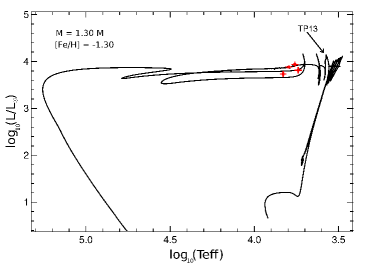
Figure 1: HR diagram showing the evolution of our 1.3 ${\mathrm{M}_{\sun}}$, [Fe/H$]=-1.3$ model from the start of the main sequence to the white dwarf cooling track. The locations of the four post-AGB stars are represented by the red dots with error bars. The location of the third last thermal pulse (TP13) is also indicated. (The color version of this figure is available in the online journal.)

Table 1: Properties of the ¹³C-pocket models. M_TDU is given for the models that include only one ¹³C pocket.

	Yp	13C burninga	MPMZ(${\mathrm{M}_{\sun}}$)	M${}_{\rm p}^{\rm tot}$(${\mathrm{M}_{\sun}}$)	artificial MTDU(10-3 ${\mathrm{M}_{\sun}}$)
					J004441	J050632	J052043	J053250
pocket_case1	$standard^{b}$	radiative	$1.8\times 10^{-3}$	$1.35\times 10^{-4}$	45.3	1.05	3.13	4.16
pocket_case2	$standard^{b}$	convective	$1.0\times 10^{-3}$	$7.50\times 10^{-5}$	3.77	0.18	0.51	0.67
pocket_case3	$0.70\times 10^{-4}$	radiative	$1.8\times 10^{-3}$	$1.26\times 10^{-7}$	87	1.33	4.03	5.40
pocket_case4	$1.05\times 10^{-4}$	radiative	$1.8\times 10^{-3}$	$1.89\times 10^{-7}$	6.04	0.27	0.78	1.02
pocket_case5	$1.05\times 10^{-4}$	radiative	$3.6\times 10^{-3}$	$3.78\times 10^{-7}$	2.76	0.14	0.39	0.50

Figure 2: Proton abundance distribution artificially inserted during the post-processing in our models to simulate the formation of a ¹³C pocket after the 12^th TP (left panel) and a PIE event during TP13 (right panel). Left panel: The thin line represents the standard exponentially decreasing proton distribution (pocket_case1) and the thick line the case where the proton abundance Y_p is set to constant equal $1.05\times 10^{-4}$ (pocket_case4). The dotted line represents the depth reached by the TDU. Right panel: The thin and thick lines represent two different proton distributions with a similar total amount of protons ingested: PIE_case1 (thin line) and PIE_case2 (thick line). The dotted line represents the maximum extention of the intershell convective region associated with TP13. The steep proton profile left over by the H-burning shell is also shown in the plot just above 0.638 ${\mathrm{M}_{\sun}}$.

The proton abundance distribution used in pocket_case1 (thin line of left panel in Fig. 2) is the same or very similar to the choice made in the models presented by De Smedt et al. (2012, 2014) and, as expected, produces the same results. According to our stellar evolution model the ¹³C always burns completely before the onset of the following TP. In pocket_case2 we experimented with artificially keeping the temperature below 70 MK in the pocket, which is not enough to activate the ¹³C($\alpha$,n)¹⁶O reaction. A much lower value of the rate of this reaction is excluded since it is known within a factor of $\sim$4 (Bisterzo et al., 2015), but it is possible that a TDU episode leading to the formation of the ¹³C pocket occurred in the earlier pulses, when the core mass and the temperature are lower. In fact, the core mass at which the TDU begins is uncertain and may be lower than in our model (Kamath et al., 2012). For example, if the first TDU episode occurred after the 2^nd instead of the 8^th TP the temperature in the region of the ¹³C pocket would not have exceeed 70 MK before the development of the next TP. In this case the neutrons are released inside the following TP as the ¹³C is ingested. Next, we set the proton abundance Y_p to be constant with values equal to $0.70\times 10^{-4}$ (pocket_case3) or $1.05\times 10^{-4}$ (pocket_case4, thick line of left panel of Fig. 2, and pocket_case5). Physically, this may correspond to efficient mixing inside the ¹³C pocket during the interpulse period induced by the difference in the angular momentum between the core and the envelope in a rotating AGB star. This mixing carry the neutron poison ¹⁴N into the ¹³C-rich layers (e.g., Piersanti et al., 2013), lowering the $s$-process efficiency. However, the actual effect is uncertain because magnetic fields can slow down the core by coupling it to the envelope, and inhibit mixing. In the radiative ¹³C-pocket pocket_case4 the neutron flux lasts for roughly 30,000 yr, the total time-integrated neutron flux (neutron exposure) is $\simeq$0.5 mbarn^-1, and the neutron density reaches a maximum of $5.2\times 10^{6}$ cm^-3. In the case of the convective ¹³C pocket (pocket_case2) the neutron flux lasts for a much shorter time, of the order of 10 yr, and the neutron density reaches a much higher maximum of $2.5\times 10^{11}$ cm^-3 for a similar neutron exposure.

Table 2: Properties of the PIE models.

	Y${}_{\rm p}^{\rm max}$	M${}_{\rm ext}^{a}$(${\mathrm{M}_{\sun}}$)	M${}_{\rm p}^{\rm tot}$(${\mathrm{M}_{\sun}}$)	MTDU($10^{-3}$ ${\mathrm{M}_{\sun}}$)
				J004441	J050632	J052043	J053250
PIE_case1	0.035	$8.0\times 10^{-4}$	$4.48\times 10^{-6}$	0.68	0.03	0.10	0.13
PIE_case2	0.007	$3.5\times 10^{-3}$	$5.25\times 10^{-6}$	1.08	0.06	0.16	0.20
PIE_case3	0.007	$4.0\times 10^{-3}$	$6.0\times 10^{-6}$	0.41	0.02	0.06	0.08

We also run some preliminary tests to simulate a proton-ingestion episode (PIE) during the post-processing by inserting an artificial proton abundance distribution in the intershell before the convective zone of TP13 reaches its maximum extension. At this time the H shell is completely extinguished. These protons are ingested as the convective region extends outward. As in the ¹³C-pocket models, we artificially simulated a single last TDU event mixing the material from the He intershell into the envelope after TP13 had subsided, setting the amount of TDU mass to the value required to match the observed [La/Fe]. Table 2 shows the main features of the PIE models, where Y${}_{\rm p}^{\rm max}$ is the maximum proton abundance, M_ext the mass extent of the p-rich region, M${}_{\rm p}^{\rm tot}$ the total integrated mass of protons, and M_TDU the TDU mass required to match each star. The M_TDU required in the PIE models are typically lower than in the ¹³C-pocket models.

The proton abundance distribution is set to exponentially decrease with mass from a value Y${}_{\rm p}^{\rm max}=0.035$ (PIE_case1, thin line of right panel of Fig. 2) or 0.007 (PIE_case2, thick line of right panel of Fig. 2 and PIE_case3) to a value of 10^-4 over M_ext. The protons are ingested in the convective region and captured by ¹²C, which results in the production of ¹³C and subsequently of free neutrons for the $s$ process via ¹³C($\alpha,$n)¹⁶O. We ran a series of models varying the total mass of protons ingested M${}_{\rm p}^{\rm tot}$ and found best solutions for M${}_{\rm p}^{\rm tot}=4.5-6\times 10^{-6}$ ${\mathrm{M}_{\sun}}$ ,i.e., M${}_{\rm ext}=0.8-4\times 10^{-3}$ ${\mathrm{M}_{\sun}}$, depending on Y${}_{\rm p}^{\rm max}$. This mass extent is relatively large: a more realistic profile to simulate overshoot of the convective intershell region into the proton tail left over by the H-burning shell would have a higher Y${}_{\rm p}^{\rm max}$ (e.g, $\sim 0.2$) and a much smaller M_ext ($\sim 10^{-5}$ ${\mathrm{M}_{\sun}}$, see Fig. 2). However, to set and follow such a profile appropriately requires very high temporal and spatial resolution, leading to extremely long running times with our computational tools. We leave this task to future work.

In comparison to the scenario of the ¹³C pocket, the neutron flux lasts for a very short time, of the order of 10^-1 yr, five orders of magnitudes shorter than in the radiative ¹³C pocket, while the neutron density reaches a maximum of $5\times 10^{13}$ cm^-3 (e.g., in the PIE_case2 model), seven orders of magnitude higher than in the radiative ¹³C pocket. Even at this value of the neutron density, the neutron-capture path does not move further away from the valley of $\beta$ stability by more than two or three atomic mass numbers, for each given element, and still proceeds sequentially throughout each value of the proton number.

Finally, because the PIE was included in the post-processing calculations only, we cannot evaluate its feedback on the stellar structure and evolution. PIEs can lead, for example, to a splitting of the convective region, as energy released by H burning creates a temperature inversion inside the convection zone. The amount of protons ingested in our model is small (up to $6\times 10^{-6}$ ${\mathrm{M}_{\sun}}$) but this has been found in some PIE models to be enough to start the splitting of the convective zone (Miller Bertolami et al., 2006; Herwig et al., 2011). However, this effect is model dependent, e.g., the 3D PIE models of Stancliffe et al. (2011) do not find the split to occur even for larger amounts of protons, while the 3D PIE models of Woodward et al. (2015) do. The method we have used to simulate a PIE is clearly artificial and preliminary, but any 1D model not considering hydrodynamics is necessarily inaccurate, and also 3D PIE models are not in agreement with each other. Nevertheless, the usefulness of our approach lies in the opportunity of identifying major qualitative differences between the PIE and the ¹³C-pocket scenarios.

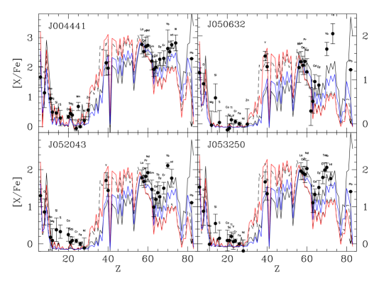
Figure 3: [X/Fe] ratios as a function of the atomic number Z predicted at the stellar surface by the models where one ¹³C pocket is introduced at the end of the TDU episode after the 12^th TP as compared to the observations of each of the four post-AGB stars indicated in the panels. We normalise both model predictions and observations to meteoritic rather than photospheric solar abundances for the elements heavier than Fe (Asplund et al., 2009). Notably, this modifies the observed [Pb/Fe] upper limits reported by De Smedt et al. (2014) by $-$0.3 dex. The black line represents pocket_case1, which produces a similar pattern as that presented by De Smedt et al. (2014) with a corresponding high Pb abundance. pocket_case2 is shown as a black dashed line. The colored lines represent pocket_case3 (red) and pocket_case4 (blue). (The color version of this figure is available in the online journal.)

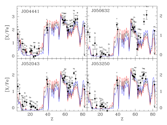
Figure 4: Same as Fig. 3 but for the PIE models. The black line represents PIE_case1 (Table 2) and the two colored lines represent PIE_case2 (red) and PIE_case3 (blue). (The color version of this figure is available in the online journal.)

3 Results

If protons are introduced after each of the five TDU episodes computed by the stellar evolution code it is not possible to find a solution for any of the four stars since the predicted [Pb/Fe] for the models that match [Zr/Fe] is always above the observed upper limit (by +0.2 dex for J050632 and by +0.6 for the other three stars). When we include only one ¹³C pocket, instead, the production of Pb is lower and it is possible to find a case that simultaneously matches [Zr/Fe] and [Pb/Fe] (Fig. 3). The reason for this difference is that with more ¹³C pockets the material is recurrently exposed to several neutron fluxes, which pushes the abundance pattern towards Pb. In pocket_case2 M_PMZ controls the total amount of ¹³C ingested and consequently the neutron exposure. The best fit to the observations was found using M${}_{\rm PMZ}=10^{-3}$ ${\mathrm{M}_{\sun}}$. A main difference in the results between the convective and the radiative models is that the [Rb/Fe] ratio (at Z=37) is similar to [Zr/Fe] in the convective case while it is 1 dex lower than [Zr/Fe] in the radiative case. This is due to the higher neutron density, which favours the activation of the branching point at ⁸⁶Rb producing the neutron magic ⁸⁷Rb (van Raai et al., 2012; Karakas et al., 2012). The PIE model results are shown in Fig. 4. Because the general $s$-process elemental abundance pattern is a one-to-one function of the neutron exposure, it is possible to obtain very similar results in the PIE models to the ¹³C-pocket models by setting the amount of ingested protons to obtain a similar amount of free neutrons. As in the case of convective ¹³C pocket, [Rb/Fe] is close to [Zr/Fe] in the PIE cases due to the high neutron density. Observations of this element would be a powerful tool to distinguish between the different scenarios, however, it is difficult to estimate its abundance in these stars because it presents only one very strong line, which is saturated.

The ¹³C-pocket models typically predict higher [C/Fe] ratios than observed, however, this result depends on M_PMZ. For example, in pocket_case5 we doubled M_PMZ and matched the observed [C/Fe], within the error bars, for the three LMC stars. To match the [C/Fe] in J004441, instead, requires a tenfold increase of the mass of the ¹³C pocket, which would cover the whole intershell. Extra-mixing phenomena at the base of the envelope during the red giant and AGB phases could remove C to produce N. Using the upper limit of the observed C abundance, the results for pocket_case5, and assuming that the excess C is converted into N via extra mixing, we expect [N/Fe] in J004441 to be greater than 2.5 dex. This is two orders of magnitude larger than the value of $0.61\pm 0.5$ derived by De Smedt et al. (2014). The PIE models, instead, typically predict lower [C/Fe] ratios than observed, due to the lower M_TDU. The O abundances are generally underestimated by all the models, which indicates that a higher O abundance must be present in the intershell and could be achieved if the timescale of He burning during the TPs was longer or if some mixing occurred between the base of the convective zone and the C-O core (Herwig, 2000).

The four stars show positive [Y/Zr] while all the models predict negative values. We do not pursue this issue further because there may be a systematic error in the observations since the Y abundance is often based on a limited number of spectral lines. Another serious problem is that the models that produce [Pb/Fe] below the observational upper limits together with Y and Zr reasonably close to the observations underproduce the abundances of the elements between Eu and Pb, such as Eu, Dy, Er, Lu, Yb, Hf, and W. The number of lines used to determine the abundances of these elements are limited and often blended, however, we cannot ascribe the mismatch to observational issues since all the four stars clearly show this problem for several of these elements.

4 Discussion and conclusions

It is not possible for the $s$ process to produce high abundances of the elements from Eu to W together with a Pb deficiency. This is because once the bottleneck at the nuclei with magic number of neutrons 82 (¹³⁸Ba and ¹³⁹La) is bypassed the neutron-capture flux proceeds through each isotope to ²⁰⁸Pb according to its neutron-capture cross section. In other words, the abundance pattern between the magic neutron numbers at Ba and Pb is almost completely determined by the neutron-capture cross sections of the isotopes involved. These are relatively well known (Bao et al., 2000) and that their values cannot be drastically changed is also demostrated by the fact that the $s$-process has no major problems (within 10-20%) in reproducing the solar system abundances of nuclei between Ba and Pb that are exclusively produced by the $s$-process. These are $s$-only nuclei such as ¹⁵⁴Gd, ¹⁶⁰Dy, and ¹⁷⁰Yb, which typically contribute only a few percent to the total abundance of the element in the solar system (Arlandini et al., 1999; Bisterzo et al., 2011).

Further observational constraints are available for a number of CEMP stars, which have metallicity roughly a factor of ten lower than the post-AGB stars considered here and are believed to have accreted $s$-process material from a more massive binary companion that evolved through the AGB phase. Bisterzo et al. (2012) compared CEMP-$s$ stars (showing enhancements in the typical $s$-process element Ba) to AGB $s$-process models. They also included initial enhancements up to 2 dex in the $rapid$ neutron-capture process (the $r$-process) elements to match the Eu abundances of CEMP-$s$/$r$ stars (showing enhancements in both Ba and the typical $r$-process element Eu). The $s$-process models give a reasonable fit to the observations of all CEMP-$s$ stars for which at least one element between Eu and Pb is observed (CS 22964-161, CS 22880-074, CS 29513-032, CS 22942-019, CS 30301-015, CS 30322-023, and HD 196944). Four out of nine CEMP-$s$/$r$ stars with observations for the elements between Eu and Pb (CS 22898-027, CS 29497-030, HE 0338-3945, and HE 2148-1247) can also generally be matched by the models. The remaining five CEMP-$s$/$r$ stars with observations for several elements between Dy and Pb (SDSS J1349-0229, CS 31062-050, LP 625-44, SDSS J0912+0216, and HD 209621), instead, cannot be matched by the models because, as for the post-AGB stars discussed here, the observed abundances are too high even if the initial $r$-process abundances are enhanced.

As suggested for CEMP-$s$/$r$ stars (Lugaro et al., 2012), an $s$/$r$ neutron-capture process intermediate between the $s$ and the $r$ process may have shaped the abundance pattern in the post-AGB stars. There are no detailed models of this process yet for low-metallicity AGB stars, though PIE events have been identified as a a possible physical site (the $i$ process, Cowan & Rose, 1977; Herwig et al., 2011). Overshoot leading to PIEs is uncertain, but known to be favoured in AGB stars of mass $\sim$ 1 ${\mathrm{M}_{\sun}}$ and [Fe/H]$<$2 (Fujimoto et al., 1990; Campbell & Lattanzio, 2008; Cristallo et al., 2009; Lugaro et al., 2012) with recent 3D models supporting these results (Stancliffe et al., 2011; Herwig et al., 2014; Woodward et al., 2015). We stress that one-dimensional hydrostatic models of PIE events with artificial proton distributions like those presented here are not expected to describe the ingestion and the mixing correctly and this may have a strong effect on the resulting abundance patterns. However, our 1D models are still informative. For example, we expect that the overabundance of Rb found in our PIE models may be a prominent feature also in more accurate, e.g., 3D, PIE models (Herwig et al., 2011). Furthermore, the dilution of intershell material into the envelope required to match the observations cannot be substantially different from that we have found here; and to avoid overproduction of Pb, also the amount of protons ingested during a PIE cannot be substantially different. For example, taking J053250 and comparing it with the model predictions from the PIE model that ingested $6\times 10^{-6}$ ${\mathrm{M}_{\sun}}$ of protons, we could match the observations by converting roughly 2/3 of the predicted Pb abundance into abundances of the elements between Eu and Pb. In other words, a match to the observations would require the same amount of free neutrons that we have in our models, but, distributed differently among the elements between Eu and Pb. This may be possible if the neutron density was a few orders of magnitude higher than in our models and the path of neutron captures was shifted further away from the valley of $\beta$ stability, as in the $i$ process.

The fact that all four post-AGB stars of low mass considered here show similar abundance patterns in the elements heavier than Fe suggests that the $i$ process may be a common occurrence in low-mass AGB stars up to [Fe/H]$\sim$1. Since stars in this mass range are common this would have important implications for the stellar yields that drive the chemical evolution of stellar clusters and galaxies. For example, these long-lived low-mass stars may be the $i$-process source required to match observations of [Ba/Fe] and [Ba/La] overabundances in open clusters (Mishenina et al., 2015). If the $i$ process is confirmed to be responsible for the abundances observed in CEMP-$s$/$r$ and post-AGB stars similarities and differences in the neutron-capture pattern of the two groups, which sample different metallicity ranges, will provide fundamental constraints to pin down its metallicity dependence and its impact on the chemical evolution of stellar systems.