Optimal lengthscale for a turbulent dynamo

Abstract

We demonstrate that there is an optimal forcing length scale for low Prandtl number dynamo flows, that can significantly reduce the required energy injection rate. The investigation is based on simulations of the induction equation in a periodic box of size $2\pi L$. The flows considered are turbulent ABC flows forced at different forcing wavenumbers $k_{f}$ simulated using a subgrid turbulent model. The critical magnetic Reynolds number $Rm_{c}^{T}$ decreases as the forcing wavenumber $k_{f}$ increases from the smallest allowed $k_{min}=1/L$. At large $k_{f}$ on the other hand, $Rm_{c}^{T}$ increases with the forcing wavenumber as $Rm_{c}^{T}\propto\sqrt{k_{f}}$ in agreement with mean-field scaling prediction. At $k_{f}L\simeq 4$ an optimal wavenumber is reached where $Rm_{c}^{T}$ obtains its minimum value. At this optimal wavenumber $Rm_{c}^{T}$ is smaller by more than a factor of ten than the case forced in $k_{f}=1$. This leads to a reduction of the energy injection rate by three orders of magnitude when compared to the case that the system is forced in the largest scales and thus provides a new strategy for the design of a fully turbulent experimental dynamo.

Dynamo is the mechanism by which magnetic fields are amplified in stars and planets due to their stretching by the underlying turbulent flow Moffatt (1978). In the last two decades several experimental groups have attempted to reproduce the dynamo instability in the laboratory Gailitis et al. (2001); Stieglitz and Müller (2001); Monchaux et al. (2007). The first successful dynamos were achieved in Riga Gailitis et al. (2001) and Karlsruhe Stieglitz and Müller (2001). The flow in these dynamos were highly constrained and did not allow for turbulence to fully develop at large scales. The first fully turbulent dynamo was achieved in Monchaux et al. (2007) where the flow was driven by two counter rotating propellers. However, in this experiment dynamo was only obtained when at least one ferromagnetic iron propeller was used. So far other attempts to achieve dynamo are not successful and unconstrained dynamos driven just by the turbulent flows have not been achieved.

One of the major difficulties to achieve liquid metal dynamos are the low values of magnetic Prandtl numbers $P_{{}_{M}}$ (the ratio of viscosity $\nu$ to magnetic diffusivity $\eta$) that characterizes liquid metals and is less than $10^{-5}$. This implies that very large values of the Reynolds number $Re=UL/\nu$ (where $U$ is the rms velocity and $L$ is the domain size) are needed to reach even order one values of the magnetic Reynolds numbers $Rm=UL/\eta=P_{{}_{M}}Re$. The magnetic Reynolds number is the critical parameter that determines the dynamo onset. For small values of $Rm$ no dynamo instability exists and $Rm$ should be larger than a critical value $Rm_{c}$ in order to generate the spontaneous growth of the magnetic field. The large $Re$ needed to reach values of $Rm$ above $Rm_{c}$ imply large power consumption that scales like $I\propto\rho U^{3}L^{3}/\ell_{f}$ (where $\ell_{f}$ is the length scale of the forcing).

The dependence of the dynamo threshold $Rm_{c}$ on the Prandtl number was investigated by different groups Ponty et al. (2005); Mininni (2007); Schekochihin et al. (2005); Iskakov et al. (2007) for different flows with the use of numerical simulations. These studies showed that as the magnetic Prandtl number is decreased the critical magnetic Reynolds number is initially increased. The turbulent fluctuations generated at large values of $Re$ inhibit dynamo action raising the critical power to values much larger than in the case of more organized laminar flows. However when sufficiently large Reynolds numbers are reached this increase saturates and a finite value of $Rm_{c}$ is reached in the limit of $Re\to\infty$. We will refer to this value as the turbulent critical magnetic Reynolds number and define it as $Rm_{c}^{T}\equiv\lim_{Re\to\infty}Rm_{c}$. The afore mentioned studies managed to reach this asymptote only by using subgrid scale models (either hyperviscocity, $\alpha$ model LES, or a dynamical turbulent viscosity) that model the high Reynold number flows. It is worth pointing out that the different flows considered led to different values of $Rm_{c}^{T}$ implying that it is possible to optimize the flow to reduce $Rm_{c}^{T}$. This is what we investigate in this work by varying the length scale of the forcing $\ell_{f}$ with respect to the domain size $L$. A similar study but for laminar flows was performed in Tilgner (1997); Plunian and Rädler (2002); Plunian (2005). The study is based on the results of numerical simulations using a pseudospectral method in a triple periodic domain Gomez et al. (2005a, b) and analytic estimates based on scale separation arguments.

In their simplest form the governing equation for the evolution of the magnetic field is given by

$$\partial_{t}{\bf b}=\nabla\times({\bf u\times b})+\eta\Delta{\bf b}$$ (1)

where ${\bf b}$ is the magnetic field, and $\eta$ the magnetic diffusivity. ${\bf u}$ is the velocity field that is determined by solving the independent incompressible Navier-Stokes equation of a unit density $\rho=1$ fluid,

$$\partial_{t}{\bf u}+({\bf u\cdot\nabla u})=-\nabla P+\nu\Delta{\bf u}+{\bf f}.$$ (2)

where ${\bf f}$ is an external forcing. In the present study the domain considered is a triple periodic box of size $2\pi L$ and $\bf f$ is taken to be the ABC forcing

$${\bf f}=\left[\begin{array}[]{c}A\sin(k_{f}z)+C\cos(k_{f}y),\\ B\sin(k_{f}x)+A\cos(k_{f}z),\\ C\sin(k_{f}y)+B\cos(k_{f}x)\end{array}\right]$$

with $A=B=C=1$. $k_{f}$ is the forcing wave number, and we define the forcing lengthscale as $\ell_{f}\equiv k_{f}^{-1}$. The ABC flow has been the subject of many dynamo studies both in the laminar Childress (1970); Alexakis (2011) and turbulent state Mininni (2007).

In this set up some analytical progress can be made in the case that $k_{f}L\gg 1$. Then one can use standard mean-field approximations to estimate the critical onset $Rm_{c}^{T}$ Parker (1955); Steenbeck et al. (1966); Childress (1970). Splitting the magnetic field in a large scale component $\bf B$ and a fluctuating part $\tilde{\bf b}$ for scale separation we obtain to first order for the fluctuating field

$$\eta\Delta\tilde{\bf b}=-{\bf B\nabla u}$$ (3)

and for the large scale field

$$\partial_{t}{\bf B}=\nabla\times(\alpha{\bf B})-\eta\Delta{\bf B}$$ (4)

where $\alpha$ is a tensor such that $\alpha_{ij}B_{j}=\langle{\bf u\times\tilde{\bf b}}\rangle_{i}$ the angular brackets stand for small scale average and summation over the index $j$ is implied. For the particular forcing chosen the $\alpha$-tensor is diagonal and isotropic. The non-zero diagonal elements $\alpha_{ii}$ can be calculated by solving (3) for a given velocity field and are

$$\alpha_{ii}=\frac{-1}{\eta}\langle{\bf u}\times\Delta^{-1}\nabla_{i}{\bf u}\rangle_{i}=a\frac{U^{2}}{\eta k_{f}},$$ (5)

(no summation over $i$ is implied). $a$ is the non-dimensional $\alpha_{ii}$ element that is independent of $U,\eta$ and $k_{f}$ and needs to be calculated from the flow. The growth rate $\gamma$ for a helical large-scale mode of wavenumber $K=1/L$ is then

$$\gamma=a\frac{U^{2}}{\eta k_{f}L}-\eta L^{-2}$$ (6)

that leads to a critical Reynolds number $Rm_{c}=\sqrt{k_{f}L/a}$. This result was discussed in Fauve and Pétrélis (2002). Note that this argument is true both for turbulent and laminar flows although the value of the coefficient $a$ will depend on the level of turbulence. At large $Re$ however $a$ will reach an asymptotic value $a^{{}_{T}}$ that will determine the value of $Rm_{c}^{T}$ to be

$$Rm_{c}^{T}=\sqrt{k_{f}L/a^{{}_{T}}}.$$ (7)

This scaling implies that in the large scale separation limit $k_{f}L\gg 1$ for fixed $L$ and $\eta$ as $k_{f}$ is increased it becomes more difficult to obtain a dynamo.

To calculate $Rm_{c}^{T}$ in the absence of scale separation we performed numerical simulations varying the forcing wavenumber $k_{f}$ for fixed $L$ of equations 1,2. In order to mimic the large Reynolds number flow that requires large grid size $N$ we do not use an ordinary viscosity $\nu$ for the dissipation but rather a dynamical wavenumber-dependent turbulent viscosity Chollet and Lesieur (1981) defined in spectral space as

$$\nu_{{}_{T}}(k,t)=0.27[1+3.58(k/k_{c})^{8}]\sqrt{E_{{}_{K}}(k_{c},t)/k_{c}}$$ (8)

where $k=|{\bf k}|$ is the wavenumber, $k_{c}=N/3L$ is the maximum wavenumber after de-aliasing and $E_{{}_{K}}(k,t)$ is the kinetic energy spectrum of the flow. The same modeling was also used in Ponty et al. (2005) to obtain $Rm_{c}^{T}$. $\nu_{{}_{T}}$ depends on the grid size $N$, but the dependence of the large scale components of the flow on $N$ are expected to die off much faster than in the case of ordinary viscosity.

To calculate $Rm_{c}^{T}$ as a function of $k_{f}$ the following procedure was used (see also Ponty et al. (2005); Iskakov et al. (2007)): For a given $k_{f}$ and grid size $N$ a series of simulations were performed varying $Rm$ and the exponential growth rate of the magnetic energy was measured. The onset $Rm_{c}$ was determined by linearly interpolating the values of $Rm$ between the slowest growing dynamo and the slowest decaying dynamo. The series of runs was then repeated for higher values of $N$ until either the value of $Rm_{c}$ remained unchanged in which case this determined $Rm_{c}^{T}$ or we reached the maximum of our attainable resolution. Typically convergence was reached at grid sizes $N=256$ but a few runs at $N=512$ were also performed for verification. In addition we solved equation 3 (with $\bf u$ given by equation 2) with an imposed uniform magnetic field to calculate the elements of the $\alpha$ tensor and determine $a^{{}_{T}}$.

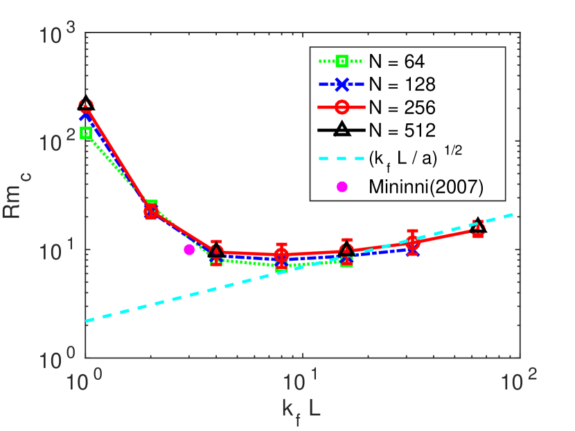
Figure 1: $Rm_{c}$ as a function of $k_{f}L$ obtained from numerical simulations of different resolutions $N=64-512$. The data indicate that for $N\geq 128$, $Rm_{c}$ does not vary as $N$ is increased further and thus it approximates well $Rm_{c}^{{}_{T}}$. The error-bars correspond to the maximum/minimum value of $Rm$ for which we obtained a clear positive/negative growth rate for the simulations with $N=256$. The filled circle corresponds to the value of $Rm_{c}^{{}_{T}}$ obtained from direct numerical simulations in Mininni (2007). The dashed line shows the mean field (alpha) prediction valid in the limit $kL\to\infty$.

The results for the critical Reynolds number as a function of the forcing wave number $k_{f}$ are shown in figure 1. The predicted scaling behavior (7) is shown with a dashed line in the same figure 1. The black dot indicates the the value of $Rm_{c}^{T}$ calculated in Mininni (2007) using simulation of higher resolutions and $\alpha$-model LES.

The results are very motivating for future laboratory experiments. Although for large $k_{f}L$ the asymptotic scaling of (7) seems to be verified indicating that making the forcing length scale very small will not benefit dynamo experiments, at intermediate length scales $Rm_{c}^{T}$ appears to reach a minimum around $k_{f}L=4$ to $8$. In fact the value of $Rm_{c}^{T}$ at this optimal wavenumber is one order of magnitude smaller than the value of $Rm_{c}^{T}$ at $k_{f}L=1$.

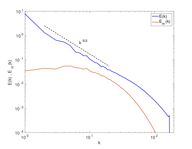
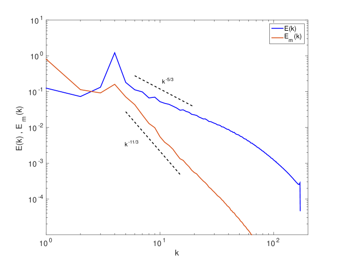
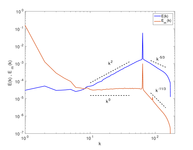
Figure 2: Kinetic $E(k)$ and magnetic $E_{m}(k)$ energy spectra for the marginally unstable modes for $k_{f}L=1$ (top), $k_{f}L=4$ (middle), $k_{f}L=64$ (bottom).

The kinetic and magnetic energy spectra for slowest growing mode for three different forcing wave-numbers at highest resolution $N=512$ are shown in the three panels of figure 2. For the case that the flow is forced in the largest scale $k_{f}L=1$ the kinetic energy shows a clear $k^{-5/3}$ spectrum while no clear power law scaling can be observed for the magnetic field. Most of the magnetic energy is concentrated in the small scales with very weak energy in the largest scale.

At the other extreme where the flow is forced in the small scales $k_{f}L=64$ most of the kinetic energy is in the small scales with a $k^{-5/3}$ scaling in the sub-forcing scales and a $k^{2}$ power-law scaling for the scales larger than the forcing scale, suggesting equipartition of energy among all modes as equilibrium statistical mechanics predict Kraichnan (1973). In addition a small peak at large scales $kL\simeq 1-2$ is observed. The $k^{2}$ energy spectrum has been observed before in numerical simulations of the truncated Euler equations Krstulovic et al. (2009), and more recently in simulations forced in the small scale where the excess of energy in the largest scale of the system has also been observed Gopalakrishnan Ganga Prasath et al. (2014); Dallas et al. (2015). The role and cause of this peak and its effect on dynamo is the subject of current investigations. The magnetic field on the other hand has a dominant peak at $kL=1$, caused by the $\alpha$ dynamo that is followed by a flat spectrum $k^{0}$, a peak at the forcing scale and then by a $k^{-11/3}$ power law until the dissipation scales. The two peaks at $kL=1$ and $k=k_{f}$ are in agreement with the mean field dynamo prediction. The two power-laws can also be explained by a balance between the stretching rate $S$ of the large scale field ${B_{{}_{L}}}$ by the fluctuations $u_{\ell}$ that is proportional to $S\propto{B_{{}_{L}}}u_{\ell}/\ell$ and the Ohmic dissipation that is proportional to $\eta b_{\ell}/\ell^{2}$. Substituting $u_{\ell}\propto\ell^{1/3}$ for the turbulent scales and $u_{\ell}\propto\ell^{-3/2}$ for the scales in equipartition one recovers the two exponents $k^{-11/3}$ and $k^{0}$ respectively. The $k^{-11/3}$ spectrum was predicted in Golitsyn (1960); Moffatt (1961) and has been observed in experiments Odier et al. (1998) and numerical simulations Ponty et al. (2004). The flat spectrum $k^{0}$ up to our knowledge is reported for the first time here.

The case $k_{f}L=4$ that is close to the optimal wavenumber seems to be somewhere is between the two extreme cases. The magnetic field at the largest scale appears neither dominant as in the mean field case bu nor negligible as in the $k_{f}L=1$ case. In the large scales there is not enough scale separation to observe any power-law, but in the small scales a power law close to $k^{-5/3}$ for the kinetic spectrum and $k^{-11/3}$ for the magnetic spectrum can be seen.

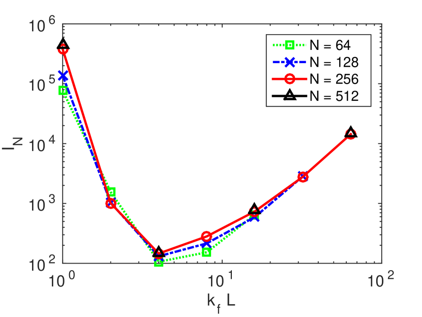
Figure 3: The non-dimensional critical injection rate $I_{N}$ as a function of $k_{f}L$.

Our results have shown that future dynamo experiments can benefit from forcing at scales smaller than the domain size by a factor of 4 to 8. To further demonstrate this fact in figure 3 we plot the minimum energy injection rate $I=(2\pi L)^{3}\langle{\bf f\cdot u}\rangle$ to achieve dynamo, normalized by the domain size $L$, the mass density $\rho$ and magnetic diffusivity $\eta$ $I_{N}=IL/(\rho\eta^{3})$. The reason we have chosen this non-dimensionalization is because the mass density and magnetic diffusivity are properties of the liquid metals that vary only with temperature, while the domain size is typically fixed. In other words by normalizing it this way we ask the question: in a laboratory experiment of a given the domain size what is the optimal forcing scale to achieve dynamo with a minimal the energy injection rate?.

The result is very encouraging! The optimal injection rate is almost three orders of magnitude smaller than the case for which the forcing was in the largest scale. This large drop in the injection rate can be partly explained by considering the turbulent scaling for the energy injection rate $I\propto\rho U^{3}L^{3}/\ell$. Substituting $U$ from the definition of $Rm$ we obtain $I\propto\rho Rm^{3}\eta^{3}/\ell$ and thus $I_{N}\propto Rm^{3}k_{f}L$. Thus the energy injection rate is very sensitive on changes in $Rm$ and the beneficial factor of 20 that was observed in figure 1 translates to a factor 2000 for the energy injection rate. It is also worth pointing out that the while for optimizing $Rm_{c}^{{}_{T}}$ the optimal forcing wavenumber was between $k_{f}L=4$ and $k_{f}L=8$, in the case that $I_{N}$ is optimized the optimal wave number is more clearly the $k_{f}L=4$.

In the light of this result we can envision the design of new dynamo experiments where the flow is forced by an array of propellers so as to result in the small scale forcing required. Such experiments will challenge long standing theoretical assumptions of mean field dynamo theories.