Fast community structure local uncovering by independent vertex-centred process

Abstract

This paper addresses the task of community detection and proposes a local approach based on a distributed list building, where each vertex broadcasts basic information that only depends on its degree and that of its neighbours. A decentralised external process then unveils the community structure. The relevance of the proposed method is experimentally shown on both artificial and real data.

I Introduction

Social networks are usually represented as graphs, where each vertex is a person and each edge between two vertices reflects a particular relationship, e.g. these people know each other or share a common interest [1]. The structure of a social network graph often reveals the presence of communities, intuitively defined as subsets of vertices more densely connected within themselves than with others.

When interacting in today’s real world in this context, most people carry a wireless communication device –such as a smartphone but also so-called smart objects, such as smart watches or wearables to name a few– and constitute the vertices of a volatile ad-hoc delay-tolerant communication network known as opportunistic mobile social network, a class of Mobile Ad-hoc NETwork (MANET), and encompasses a community structure as well [2, 3]. The automatic identification of these communities can prove beneficial to better route the traffic inside that network [4].

Hui et al. [5] showed that knowing the community structure of such a network can help improving the routing of packet traffic inside it. If the network is formed through human-carried devices, thus reflecting a probable social organisation, the improvement can be significant [2, 6].

Moreover, if the emergence of a network occurs at specific place, such as a museum or a store, or during a specific event such as an exhibit or a job-dating, the live uncovered community structure can be used to offer an enhanced experience to the visitor/customer by recommending specific content or places, and thereby to increase merchant benefits. Experiments conducted at MIT where each user carries a small electronic communicating badge on their shirt show that these badges are useful to successfully live build affinity models among participants and infer interest between people [7, 8]. We believe that adding the community structure to the features used to build the models, bringing a social dimension, could improve the models quality. However, it is a difficult task and a challenging problem in the field of graph mining, as detailed in Section II. Most existing methods, at the protocol level implementation, require vertices of the network to share a certain amount of information implying many exchanges between them, or calculations requiring many inputs.

This paper proposes a simple distributed method with reduced propagation, therefore easily deployable in the context mentioned above. We show that, only by having vertices share a list based on the degrees of their neighbours, we are able to unveil a coherent community structure.

This paper is organised as follows: the next section discusses related works, Section III describes the method we propose and Section IV presents and discusses some experimental results.

II Related Works

The community detection task aims at decomposing a graph into subgraphs that are more densely connected within themselves than with others. Several formal definitions of community have been proposed[9, 10], though none is universally accepted, opening the way to many different approaches. We propose to distinguish between 2 main categories, namely global and local methods.

II-A Global Approaches

The global approaches, introduced first, initially derived from computational graph analysis, like partitioning, clustering or clique-finding [11, 12, 13].

The exploitation of graph topology analysis then led to the introduction of the modularity measure [14, 15], used in numerous algorithms, such as Clauset [16] or Louvain [17] to name two examples. Other criteria have been proposed to address the limits of modularity [18, 19]. Other approaches include techniques based on statistical models [20] or informations flows [21] for example.

However, these methods require to know the entire graph topology, imposing to dispose of the whole graph for their processing.

II-B Local Approaches

The second category, made of local approaches, detect communities by means of a local measure, processing only a subset of the graph, e.g. a subset of vertices, a subset of edges, or a subgraph. These local approaches allow an analysis portion by portion, thereby facilitating the conception of a distributed implementation. They also make it easier to process dynamic graphs, as they can adapt to local modifications of the graph [22]. In particular, they apply to the case of opportunistic networks mentioned in the introduction, such as Pocket Switched Networks [23]: in this case, community detection is difficult using a global approach because there is no central unit knowing all the network vertices at the same time.

Local approaches can be defined as variations of global methods described in the previous subsection: modularity has, for instance, been adapted for such a local exploitation [24].

Other recent local approaches include label propagation [25] and seed-centric [26]. Label propagation basically consists in assigning a label to each vertex and propagating these labels between neighbours and throughout the network following given rules. After achieving convergence, vertices labelled with the same label will be considered as belonging to the same community. However, propagation to the whole network can lead to flooding effects and can be a significant downside as opportunistic networks are often delay-tolerant so the synchronisation can be tough. Seed-centric consists in identifying a vertex or group of vertices displaying specific properties that will constitute a basis (the seed) on which the community detection is performed.

The local approach we propose, as detailed in the next section, requires little computation, no centralised process and limits the information exchange to the close neighbours.

III Proposed algorithm

This section presents the algorithm we propose, first exposing the underlying concepts, then describing each part separately and examining its properties.

We consider an undirected and unweighted graph without isolated vertices nor self-loops, denoted $G=(V,E)$, where $V$ is the set of vertices, $E$ the set of edges, $n=|V|$ and $m=|E|$, $d_{v}$ is the degree and $\Gamma(v)$ the set of neighbours of a vertex $v$. The absence of isolated vertex implies that $\forall v\in V,d_{v}>0$.

$\mathcal{C}=\{c_{1},...,c_{|\mathcal{C}|}\}$ is the set of communities formed after detection, and $C(v)$ refers to the community a vertex $v$ belongs to.

III-A Overview and Architecture

The principle on which the proposed approach relies is that, in a context where a vertex can be aware of its environment, like an electronic communicating device as mentioned above, minimal information sharing among vertices is sufficient to serve as a basis to form communities. This method does not optimise a mathematical property characterizing communities like modularity, but is well suited for use in a decentralized, mobile networking environment requiring minimal computation.

The proposed method makes the vertices perform the essential part of the computation: metaphorically, each vertex answers the question: “Which of my neighbours am I the most related to?”. This step allows to identify locally the vertex or set of vertices attracting most of their neighbours. Note that this assumption has a meaning close to the preferential attachment theory [27].

Then, the community structure uncovering process brings together the vertices that most want to be together. This process is external to the vertices, so no vertex has to propagate information to others. At the end of the uncovering process, each vertex knows its own community, but not the whole community structure of the network. This structure may be found by doing a graph traversal, or an exploration of the graph. The advantage is that only a part of the community structure can be retrieved, with a partial graph traversal or local exploration for example, adjusting the computing resources consumption to just what is needed. Indeed, the entire structure is often not required, as for the Internet: no router knows the full topology because it is too vast and too fast-changing. However, a knowledge of a subpart of the Internet is sufficient for efficiently routing the packets.

In short, the desired overall effect is first to locally identify the densest areas in the graph where the vertices of highest degree are found, and then to group together vertices around them. This approach is related to the seed-centric community detection method family, except that we do not seek to identify a seed area but rather to have the vertices know and organise themselves to reveal the community structure.

The proposed method requires little computation power and memory use: the only prerequisite is that a vertex must be able to communicate with its neighbours to get or send minimal information, for example about the degrees. The calculation is then easily distributed over the vertices themselves, i.e. the connected devices constituting network.

More precisely, the algorithm is composed of 3 steps successively detailed in the next subsections:

1. List of candidates compiling: each vertex builds a list including some of its neighbours depending on their degree. Each vertex can run this step independently, at the same time.

2. Agreement computation and assignment: in this step, each vertex $v$ shares its list with its neighbourhood. It calculates the proportion of vertices in common between its list and those of its neighbours (agreement). It selects the neighbour $a_{v}$ it has the highest agreement with.

3. Community uncovering on $\mathcal{V}$: for each pair $(v,a_{v})\leavevmode\nobreak\ \in\leavevmode\nobreak\ \mathcal{V}$, the communities of $v$ and $a_{v}$ are merged.

III-B List of candidates compiling

We think that having vertices share minimal information to their close neighbourhood is a simple yet efficient way to identify denser areas in the graph, assimilated with communities. We propose the minimal information required as an input for a vertex $v$ to be the degree of each of its direct neighbours, so $v$ disposes of $d_{v}$ pieces of information for input.

Then, each vertex $v$ keeps only its neighbours of highest degree in a list called $S_{v}$.

More precisely, we define an integer $k_{v}$ such that for each $v$, $k_{v}\leavevmode\nobreak\ \in\leavevmode\nobreak\ \llbracket 1\leavevmode\nobreak\ ...\leavevmode\nobreak\ d_{v}\rrbracket$, and an ordering function $\sigma_{v}$ such that $\sigma_{v}(i)$ is the index of the $i^{th}$ highest degree neighbour of $v$.

$S_{v}$ is then defined for $u\in\Gamma(v)$ as:

$$S_{v}=\{u_{\sigma_{v}(1)},...,u_{\sigma_{v}(k_{v})}\}$$

We discuss the value to be given to $k_{v}$ in Section IV.

The motivation behind this way of proceeding is that a vertex cannot know with certitude if it lies in the core of a dense area of the graph or in a more remote part, but can improve its knowledge with the help of information transmitted by its neighbours.

However, to avoid using massive propagation, which is the case for the label propagation based methods, we limit the information exchange, about the degree, to the immediate neighbourhood. Given the low value of diameter generally encountered in community graphs, especially inside the subgraph formed by a community, the immediate neighbourhood contains sufficient information to perform a fairly accurate detection.

III-C Agreement Computation

Once the list has been established, the next step brings together vertices that are most likely to form a community. We propose to compare the $S$ lists for each connected pair $(v,u)$, ie $S_{v}$ and $S_{u}$ for $u\in\Gamma(v)$.

The idea is that if vertices share the same neighbours in their $S_{v}$, they are more likely to be part of the same community, because the are connected to the same high-degree vertices (common neighbourhood assumption, tied with the preferential attachment theory). We assume that a vertex having fewer connection wants to join a vertex having more connections.

We thus propose to compute the agreement (agree. in short) between two neighbour vertices $u$ and $v$ as the number of vertices in common between $S_{u}$ and $S_{v}$:

$$\textrm{agreement}(u,v)=|S_{u}\cap S_{v}|$$

We then propose to associate to each vertex $v$ its neighbour with maximal agreement called $a_{v}$.

However, this choice is only relevant if the agreement is high enough, so we use a parameter $\tau\in[0,1]$ to restrict the selection of $a_{v}$ among $v$’s neighbours having a $\tau\text{-percentage}$ of agreement with it, imposing the condition that $u\in\Gamma(v),\textrm{agreement}(u,v)\geq\tau\cdot\min(d_{u},d_{v})$. If none of $v$’s neighbours fulfil an agreement greater than $\tau$, meaning that we lack information about $v$ neighbourhood, we select the $v$’s neighbour of maximal degree as it is the best alternative. So the expression of $a_{v}$ becomes:

$$a_{v}=\begin{cases}\underset{u\in\Gamma(v)}{\operatorname*{arg\,max}}\{\textrm{agree.}(u,v)\leavevmode\nobreak\ |\leavevmode\nobreak\ \textrm{agree.}(u,v)\geq\tau\cdot\min(d_{u},d_{v})\}\\ \operatorname*{arg\,max}\{d_{u}|u\in\Gamma(v)\}\leavevmode\nobreak\ \textrm{if the case above returns}\leavevmode\nobreak\ \varnothing\end{cases}$$

One of the main advantages is that, at the protocol level, any vertex $v$ needs to broadcast its list $S_{v}$ only to its neighbours for the agreement computation to be made. This property is in line with the desired limited propagation of the considered application framework.

This process is sketched in Algorithm 1.

Algorithm 1 Agreement computation and assignment

0:  vertex $v$, parameter $\tau\in[0,1]$

0:  vertex $a_{v}$, assigned vertex for $v$

1:  $v_{max}\leftarrow\operatorname*{arg\,max}\{$agreement$(u,v)|u\in\Gamma(v)\}$

2:  if agreement$(v,v_{max})\geq\tau\cdot\min(d_{v},d_{v_{max}})$ then

3:     $a_{v}\leftarrow v_{max}$

4:  else

5:     $a_{v}\leftarrow\operatorname*{arg\,min}_{u\in\Gamma(v)}s(v,u)$

6:  end if

Algorithm 2 Community uncovering

0:  set of vertices $\mathcal{V}$,

0:  set of communities $\mathcal{C}$

1:  $\mathcal{C}=\{\{v\}|v\in\mathcal{V}\}$

2:  take $v$ not processed yet

3:    merge$(C(v),C(a_{v}))$

III-D Community Uncovering

The community detection finally exploits the extracted information, namely the association of each vertex $v$ with its preferred vertex $a_{v}$. The process is initialised to a configuration where each vertex forms its own community. The next step is to merge the community of each vertex $v$ with the one of its $a_{v}$.

This process is sketched in Algorithm 2.

To do so and to minimise propagation we introduce an entity $\epsilon$ able to poll easily a certain number of vertices from an area in the graph, denoted $\mathcal{V}\subset V$. $\epsilon$ can be a high degree vertex or a dedicated unit outside the network. For example, in a smartphone ad-hoc network, $\epsilon$ can be a designated more powerful smartphone of the network or a fixed computing unit if the network is located in a closed space for example an exhibit.

$\epsilon$ then polls a vertex $v$ and merges its community with the community of its associated vertex $a_{v}$.

The community uncovering process can be distributed on multiple $\epsilon$ at the same time, thus the use of $\mathcal{V}$. As a matter of fact, $\epsilon$ just needs to have access to every vertex $v\in\mathcal{V}$, the merging being deterministic.

In order to process the whole graph, the only requirement is that the union of all considered subsets $\mathcal{V}$ equals the whole set of vertices. No condition regarding their intersection need to be applied, in particular, they do not need to be disjoint.

III-E Algorithm Properties

III-E1 Determinism

Two out of three steps are deterministic: the lists of candidates only depend on the degrees, so they remain the same for every instance of the algorithm and any order of calculation. Merging is a symmetric action, and the result does not depend on the order.

Agreement computation is not deterministic in itself; it is dependent on the order in which the vertices are considered. Also, when several candidates are suitable for an $a_{v}$, one is chosen at random. However our experimental tests show that the variations and standard deviations are minimal.

III-E2 Complexity

The list of candidates calculation process is run separately and simultaneously by each vertex $v$ and depends on the sorting of its neighbours degree. Therefore, the complexity of this process for a single vertex $v$ calculation with a $\mathcal{O}(n\cdot log\leavevmode\nobreak\ n)$ sorting algorithm can be evaluated as $\mathcal{O}(d_{v}log\leavevmode\nobreak\ d_{v})$, and as $\mathcal{O}(\bar{d}\leavevmode\nobreak\ log\leavevmode\nobreak\ \bar{d})$ on average for any $v\in V$, where $\bar{d}$ is the mean degree of the graph, for example $\frac{m}{n}$ for a balanced random graph.

Assuming that the calculations to compile the lists of candidates are distributed over the $n$ vertices, for the whole graph it takes $n\times\mathcal{O}(\bar{d}\leavevmode\nobreak\ log\leavevmode\nobreak\ \bar{d})$.

It is the same for the agreement computation, each vertex $v$ compares his $S_{v}$ list to those of its neighbours, yielding an $\mathcal{O}(d_{v}\cdot k_{v})$ complexity, and $n\times\mathcal{O}(\bar{d}\cdot\bar{k})$ for the whole graph where $\bar{k}$ is the mean $k_{v}$ over all $v\in V$. Given that $\forall v\in V,k_{v}\leq d_{v}$, we can write the complexity as $n\times\mathcal{O}(\bar{d}^{2})$. It is important to keep in mind that the calculations are run separately and simultaneously by all the vertices, thus we write the complexity that way.

Finally the community uncovering consists of a merge for each vertex considered by the process. Each process then runs in $\mathcal{O}(|\mathcal{V}|)$, and the complexity for the whole graph is $\mathcal{O}(n)$.

III-E3 Overlapping communities

In the first version of this method, we choose not to consider overlapping communities, because evaluating the quality of community structures with multiple belonging vertices is harder than those with single belonging vertices.

However, a simple way to enable the detection of overlapping communities would be to make $a_{v}$ a set and define the agreement procedure accordingly. So a vertex $v$ would join the community of each vertex in the $a_{v}$ set, instead of joining the community of a single preferred vertex $a_{v}$.

IV Experiments

This section discusses the results of experiments both on artificial and real-world graphs, to show the relevance of the proposed method, after presenting the considered quality criteria and parameter values.

IV-A Quality Criteria

We evaluate the obtained results using ARI and NMI, criteria usually applied to assess the results of clustering tasks, to compare partitions of a given set of objects.

The Adjusted Rand Index (ARI) is an enhancement of the original Rand Index corrected for chance [28]. It produces a value between $-1$ (fully incorrect match between two partitions) and $1$ (fully exact match between partitions), $0$ being, on average, the value for the comparison of two partitions obtained at random.

The Normalized Mutual Information (NMI) reflects the amount of information contained in the considered partition compared to the ground truth, normalised by the average of Shannon’s entropy of the two partitions [29]: $0$ is the value obtained for a random assignment and $1$ for a fully similar one. We use here the word “similar” because there can be a higher number of clusters in the produced result than in the ground truth, but NMI remains high as long as the obtained partition remains close to the ground truth, even if the classifier produces several clusters instead of one.

We consider ARI as a measure of whether the found communities are exactly the same (same number, same vertex partition) thus decreasing when the number of clusters differs, and NMI as a measure of how the clusters are meaningful with respect to the ground truth, ie that globally the vertices tend to be put together in both partitions even if the number of clusters is different.

IV-B Parameter Selection

The proposed algorithm depends on two parameters, $k_{v}$ and $\tau$.

We set $k_{v}=\max(1,\frac{d_{v}}{2})$, as an intermediary value. Obviously, setting $k=1$ is insufficient: a vertex would choose its $a_{v}$ to be its highest degree neighbour, but if this highest degree neighbour is not in its community, for example because $v$ lies in the border area of its community, intuitively as much linked to other communities as to vertices of its own community, it will not be placed in the most appropriate community. We experimentally found that it happens frequently, distorting the vertex partition.

On the other hand, keeping all the neighbours is not necessary: communities being considered here as denser subgraphs, a vertex is connected to the majority of its neighbours with high probability (high clustering coefficient). Moreover, the most significant neighbours bringing information, those of highest degrees, represent a small part of a vertex neighbourhood. As a matter of fact, the degrees in the whole graph are expected to follow a power-law distribution as it is really common in community networks especially social networks [27].

We experimentally set $\tau=0.2$: it appears to be the first value that achieves the best NMI, which is not improved for lower values of $\tau$.

IV-C Artificial Graphs

Artificially generated graphs allow a ground truth comparison as their properties are known by construction. We consider two generation procedures, one similar to Clauset’s [24] and the well-known LFR benchmark [30].

IV-C1 Comparison with a local approach

We start here with a comparison with another local community identification method, from Clauset. We run the same kind of experiment that he did in his paper [24].

Clauset uses generated graphs of $n=128$ vertices divided into four communities of the same size, 32 vertices each, which constitutes the ground truth. Each vertex expected degree, $z$, is the sum of the intra-community edges $z_{in}$ and inter-community edges $z_{out}$. The edges are placed independently at random between vertices so that $z,z_{in}$ and $z_{out}$ are, in expectation, respected. Clauset sets $z=16$ and makes $z_{out}$ vary, so $z_{in}=z-z_{out}$.

We compare the performance of our method to that of Clauset’s local modularity on the whole graph. Indeed, Clauset’s algorithm starts from a seed vertex in the graph and returns a community around that seed vertex, so it does not always process the whole graph at once. Clauset runs four detections processes, one for each community, and then compares the results community by community against the ground truth.

The algorithm we propose being applied to the whole graph, we had to find a way to aggregate Clauset’s algorithm results for the whole graph as well. First, we choose to run Clauset’s algorithm for each community of each graph, that is four times for each graph, selecting the seed vertex as the one having the highest degree in each community. That’s a main advantage given to Clauset’s method because it facilitates the detection, telling it where to start and omitting the fact that this method, contrary to the one we propose, cannot detect multiple communities at the same time in the graph.

Then, we aggregate the results as follows: a vertex classified in several communities is kept in only one community selected at random (as we do not consider overlapping communities here), the unclassified vertices are each put in a self-community in which they are the sole vertex, allowing a fair comparison with our method, where every vertex is assigned to only one community.

The experiment is performed for $z_{out}$ from 1 to 8, over 10 different graphs for each value of $z_{out}$. The results are presented in Figure 1. It can be observed that the performance of the method we propose is not as good as Clauset’s, except for $z_{out}=3$.

However even if the NMI remains higher for Clauset’s method than the one we propose, the ARI shows that the community partition found by Clauset is not very similar to the original one. That is because Clauset’s method classifies many vertices in several communities or not at all, so the agregation applied smoothes these results by removing the multi-affectations and adding the missing vertices, producing many single-vertex communities that do not affect much the NMI, contrary to the ARI. Our interpretation is that Clauset’s method detects well the core of each community but gets quickly lost when it goes toward the boundaries.

On the contrary, the performance of the method we propose gradually decreases but the ARI remains proportional to the NMI, showing that the meaningfulness of the community partition, compared with the original, is gradually lost and tends to resemble randomness when $z_{out}\geq 7$. As a matter of fact, the ARI compared to the original partition is more favourable for the method we propose when $z_{out}=$ 4 and 5 whereas the NMI is more favourable for Clauset’s method.

Also, we can notice that the standard deviation for Clauset’s method is high when $z_{out}=$ 2 and 3, before the performance drop, whereas the standard deviation for ours remains moderate. We interpret this as a notable instability of Clauset’s method when there is significant noise, i.e. when $z_{out}\geq 2$, leading to the performance drop.

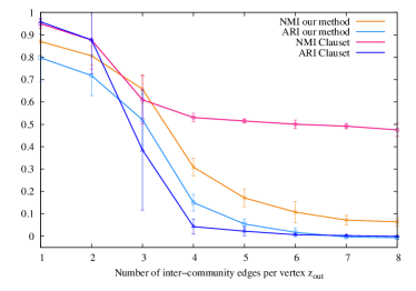
Figure 1: Average ARI and NMI for all communities over 500 generations, as compared to ground truth, for Clauset’s like graphs [24], as a function of inter-community edges $z_{out}$.

IV-C2 Comparison with global approaches

The Lancichinetti,Fortunato,Radicchi (LFR) random graphs generator [30] allows to produce better community graphs with regards to the properties of such graphs [14], than models similar to the one used by Clauset. In particular, the parameter $\mu\in[0,1]$ indicates how ”well-knit” the graph is, i.e. how much the community are clearly separated, therefore easily identifiable.

First, we run an experiment to set the best value to use for the parameter $\tau$, then we compare the method we propose to two state-of-the-art global methods: Louvain [17] and InfoMap [21].

We consider a graph with 1000 vertices for each value of $\mu$ from $0.1$ to $0.8$ increasing by $0.1$, generated by LFR, and test the algorithm we propose for different values of $\tau$.

Figure 2 shows the obtained the ARI and the NMI, mean and standard deviation averaged over 100 runs.

We can see that the method we propose performs well until $\mu=0.2$, decreasing for higher values of $\mu$, a sign of instability due to the fact that the communities become less and less identifiable.

The NMI stays higher than the ARI, meaning that for a given $\mu$, although the method we propose returns a different number of clusters than the ground truth, the partition of the vertices remains closer to the ground truth partition.

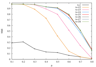
(a) NMI as a function of mixing parameter $\mu$

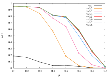
(b) ARI as a function of mixing parameter $\mu$

Figure 2: Evaluation of our method on LFR-benchmark generated graphs (1000 vertices), for different values of $\tau$.
                                                                                                                                    Curves for $\tau=\frac{1}{6}$ to $\frac{1}{8}$ are too close from each other and appear combined

Then, we compare the method we propose to Louvain and InfoMap using the value $\tau=0.2$ that yields the best results. The results, presented on Figure 3, show that the NMI stays over 0.9 until $\mu=0.5$. Louvain performs better here compared to InfoMap, which is not always the case [31], but both see their standard deviation increase, especially InfoMap for $\mu>0.5$. Although the quality of the results produced by the method we propose decreases, the advantage here is its stability (in addition to its distributed mode of operation, cf. Section III).

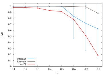
(a) NMI as a function of mixing parameter $\mu$

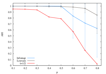
(b) ARI as a function of mixing parameter $\mu$

Figure 3: Evaluation of our method on LFR-benchmark generated graphs (1000 vertices), for different methods

Globally, as long as the community structure remains sufficiently defined ($\mu\leq 0.5$), our algorithm performs quite well as compared to global methods.

IV-D Real-world Graphs

Contrary to artificial graphs, real-world graphs are not generated after a given model but are the encoding of a real situation. They come with no ground truth, even if some of there properties are known, so the ground truth have to be human-labelled or generated by a community detection method.

IV-D1 Zachary’s Karate Club

Zachary’s karate club is a real situation [32] discussing over the conflicts leading to the separation of a karate club into two factions. The interactions between members were observed for 3 years from a sociological/ethnographic point of view. After the splitting of the initial club, the new partition was found to be strongly correlated with the interactions over the past preceding years (that was the purpose of Zachary’s paper). The two factions are seen as the 2 main communities which the graph can be divided into. It is a well-known small benchmark to study the behaviour of a community detection algorithm.

Figure 4 shows the partition made by our algorithm. The NMI and ARI for this case are 0.65 and 0.67 respectively. Three vertices are not put in the expected community compared to the partition stated by Zachary : #9, #14 and #20 (highlighted on the figure). These vertices are at the interface between the two communities and are all connected to vertex #34, one of the most influent in this community (highest degree). Therefore the classification does not seem absurd.

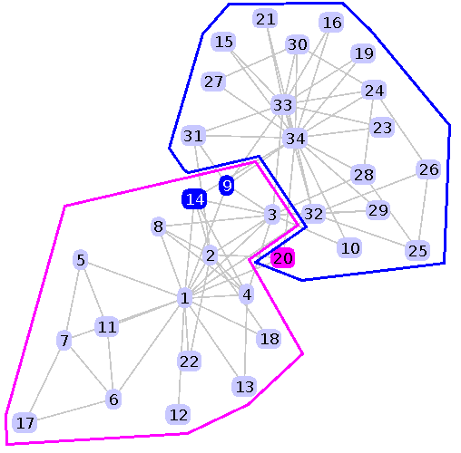
Figure 4: Community partition for Zachary’s karate club. The highlighted vertices are the only ones not compliant with the original partition.

IV-D2 Amazon

We also apply the method we propose on a co-purchasing network from Amazon.com, collected by Yang and Leskovec [33] and available online [34]. The graph has $n=334,863$ vertices and $m=925,872$ edges. It is undirected and has no isolated vertex nor self-loop. It has a clustering coefficient of approximately $0.40$, which is really low (neighbours are sparsely connected, there are few triangles). Each vertex represents a product sold on Amazon.com and each edge between two products means that they are frequently co-purchased.

The main advantage of this dataset is that it comes with a ground truth, i.e. it is possible and relevant to apply the method we propose and compare the result with the ground truth communities.

We removed from the results of our detection the vertices having no affected ground truth community, and we kept only one community at random for vertices belonging to several communities.

We achieve a NMI of 0.905, in other words our method is not only able to find communities in computer-generated graphs with controlled properties, but also in large graphs modeling -or taken from- real situations.

V Conclusion

We presented a decentralised method to detect communities on a graph, using lists based on the degrees of the vertices. The algorithm, divided in 3 steps, makes each vertex elaborate a list of defined vertices, then an agreement with the list of its neighbours. A process is run to put together vertices that have the highest agreement.

This method relies on simple calculations with few inputs, and is therefore well adapted to detect communities during a live event, where each participant carries a wireless mobile device (e.g. smartphone, smartwatch) that can do the computation and share information with other nearby devices.

We showed that this method performs well both on artificial and real graphs, although less than state-of-the-art algorithms. However, a main advantage is that it is designed to be run on a distributed architecture, more precisely over a network of connected “smart” devices e.g. smartphones. Furthermore, most of the method is deterministic, giving rather stable results, more easily predictable and more explainable.

We plan to do further experimentations with the proposed method on a larger number of graphs of various properties and models, to better understand the limits of the assignment based on agreement. Future works will also include experiments on dynamic graphs, as we think that this method is easily adaptable to the dynamic case.

Perspective also include an extension of the proposed method to the case of overlapping communities (cf. III-E3) and attributed graphs: adding other information available to constitute the lists, such as the profile of a participant carrying the device in the considered context, would greatly improve the quality of the community formation.

References

- [1] S. Wasserman and K. Faust, Social Network Analysis: Methods and Applications, 1st ed. Cambridge: Cambridge University Press, Nov. 1994.
- [2] A. Chaintreau, P. Hui, J. Crowcroft, C. Diot, R. Gass, and J. Scott, “Impact of Human Mobility on Opportunistic Forwarding Algorithms,” IEEE Transactions on Mobile Computing, vol. 6, no. 6, pp. 606–620, Jun. 2007.
- [3] N. Vastardis and K. Yang, “Mobile Social Networks: Architectures, Social Properties, and Key Research Challenges,” IEEE Communications Surveys Tutorials, vol. 15, no. 3, pp. 1355–1371, 2013.
- [4] K. Lee, P. Hui, and S. Chong, “Mobility Models in Opportunistic Networks,” in Mobile Ad Hoc Networking, S. Basagni, M. Conti, S. Giordano, and I. Stojmenovic, Eds. John Wiley & Sons, Inc., 2013, pp. 360–418.
- [5] P. Hui, E. Yoneki, S. Y. Chan, and J. Crowcroft, “Distributed Community Detection in Delay Tolerant Networks,” in Proc. of the 2007 ACM/IEEE International Workshop on Mobility in the Evolving Internet Architecture, ser. MobiArch ’07. New York, NY, USA: ACM, 2007, pp. 7:1–7:8.
- [6] P. Hui, J. Crowcroft, and E. Yoneki, “BUBBLE Rap: Social-Based Forwarding in Delay-Tolerant Networks,” IEEE Transactions on Mobile Computing, vol. 10, no. 11, pp. 1576–1589, Nov. 2011.
- [7] M. Laibowitz, J. Gips, R. Aylward, A. Pentland, and J. Paradiso, “A sensor network for social dynamics,” in Proc. of the 2006 Information Processing in Sensor Networks (ISPN), 2006, pp. 483–491.
- [8] J. A. Paradiso, J. Gips, M. Laibowitz, S. Sadi, D. Merrill, R. Aylward, P. Maes, and A. Pentland, “Identifying and Facilitating Social Interaction with a Wearable Wireless Sensor Network,” Personal Ubiquitous Computing, vol. 14, no. 2, pp. 137–152, 2010.
- [9] F. Radicchi, C. Castellano, F. Cecconi, V. Loreto, and D. Parisi, “Defining and identifying communities in networks,” Proc. of the National Academy of Sciences, vol. 101, no. 9, pp. 2658–2663, Mar. 2004.
- [10] S. Fortunato, “Community detection in graphs,” Physics Reports-Review Section of Physics Letters, pp. 75–174, Jun. 2009.
- [11] B. W. Kernighan and S. Lin, “An Efficient Heuristic Procedure for Partitioning Graphs,” Bell System Technical Journal, vol. 49, no. 2, pp. 291–307, 1970.
- [12] C. Bron and J. Kerbosch, “Algorithm 457: finding all cliques of an undirected graph,” Communications of the ACM, vol. 16, no. 9, pp. 575–577, Sep. 1973.
- [13] L. Freeman, “A Set of Measures of Centrality Based on Betweenness,” Sociometry, vol. 40, no. 1, pp. 35–41, Mar. 1977.
- [14] M. Girvan and M. E. J. Newman, “Community structure in social and biological networks,” Proc. of the National Academy of Sciences, vol. 99, no. 12, pp. 7821–7826, Jun. 2002.
- [15] M. E. J. Newman and M. Girvan, “Finding and evaluating community structure in networks,” Physical Review E, vol. 69, no. 2, p. 026113, 2004.
- [16] A. Clauset, M. E. J. Newman, and C. Moore, “Finding community structure in very large networks,” Physical Review E, vol. 70, no. 6, p. 066111, 2004.
- [17] V. D. Blondel, J.-L. Guillaume, R. Lambiotte, and E. Lefebvre, “Fast unfolding of communities in large networks,” Journal of Statistical Mechanics: Theory and Experiment, vol. 2008, no. 10, p. P10008, Oct. 2008.
- [18] R. Aldecoa and I. Marín, “Deciphering Network Community Structure by Surprise,” PLoS ONE, vol. 6, no. 9, p. e24195, Sep. 2011.
- [19] S. Fortunato and M. Barthélemy, “Resolution limit in community detection,” Proc. of the National Academy of Sciences, vol. 104, no. 1, pp. 36–41, 2007.
- [20] P. D. Hoff, A. E. Raftery, and M. S. Handcock, “Latent Space Approaches to Social Network Analysis,” Journal of the American Statistical Association, vol. 97, no. 460, pp. 1090–1098, 2002.
- [21] M. Rosvall and C. T. Bergstrom, “Maps of random walks on complex networks reveal community structure,” Proc. of the National Academy of Sciences, vol. 105, no. 4, pp. 1118–1123, Jan. 2008.
- [22] R. Cazabet and F. Amblard, “Simulate to Detect: A Multi-agent System for Community Detection,” in Proc. of the 2011 IEEE/WIC/ACM Web Intelligence and Intelligent Agent Technology (WI-IAT), vol. 2, 2011, pp. 402–408.
- [23] P. Hui, A. Chaintreau, J. Scott, R. Gass, J. Crowcroft, and C. Diot, “Pocket Switched Networks and Human Mobility in Conference Environments,” in Proc. of the 2005 ACM SIGCOMM Workshop on Delay-tolerant Networking, ser. WDTN ’05. New York, NY, USA: ACM, 2005, pp. 244–251.
- [24] A. Clauset, “Finding local community structure in networks,” Physical Review E, vol. 72, no. 2, p. 026132, Aug. 2005.
- [25] U. N. Raghavan, R. Albert, and S. Kumara, “Near linear time algorithm to detect community structures in large-scale networks,” Physical Review E, vol. 76, no. 3, p. 036106, Sep. 2007.
- [26] R. Kanawati, “Seed-centric approaches for community detection in complex networks,” in Social Computing and Social Media. Springer, 2014, pp. 197–208.
- [27] A.-L. Barabási and R. Albert, “Emergence of Scaling in Random Networks,” Science, vol. 286, no. 5439, pp. 509–512, Oct. 1999.
- [28] L. Hubert and P. Arabie, “Comparing partitions,” Journal of Classification, vol. 2, no. 1, pp. 193–218, Dec. 1985.
- [29] A. Strehl and J. Ghosh, “Cluster Ensembles — a Knowledge Reuse Framework for Combining Multiple Partitions,” Journal of Machine Learning Research, vol. 3, pp. 583–617, Mar. 2003.
- [30] A. Lancichinetti, S. Fortunato, and F. Radicchi, “Benchmark graphs for testing community detection algorithms,” Physical Review E, vol. 78, no. 4, p. 046110, Oct. 2008.
- [31] D. Hric, R. K. Darst, and S. Fortunato, “Community detection in networks: Structural communities versus ground truth,” Physical Review E, vol. 90, no. 6, p. 062805, Dec. 2014.
- [32] W. Zachary, “An information flow model for conflict and fission in small groups,” Journal of Anthropological Research, vol. 33, no. 4, pp. 452–473, 1977.
- [33] J. Yang and J. Leskovec, “Defining and evaluating network communities based on ground-truth,” Knowledge and Information Systems, vol. 42, no. 1, pp. 181–213, Oct. 2013.
- [34] J. Leskovec and A. Krevl, “SNAP Datasets: Stanford Large Network Dataset Collection,” Jun. 2014. [Online]. Available: http://snap.stanford.edu/data