Comparison between a quantum kinetic theory of spin transfer dynamics in Mn doped bulk semiconductors and its Markov limit for non-zero Mn magnetization

Abstract

We investigate the transfer between carrier and Mn spins due to the s-d-exchange interaction in a Mn doped bulk semiconductor within a microscopic quantum kinetic theory. We demonstrate that the spin transfer dynamics is qualitatively different for components of the carrier spin parallel and perpendicular to the Mn magnetization. From our quantum kinetic equations we have worked out the corresponding Markov limit which is equivalent to rate equations based on Fermi’s golden rule. The resulting equations resemble the widely used Landau-Lifshitz-Gilbert-equations, but also describe genuine spin transfer due to quantum corrections. Although it is known that the Markovian rate description works well for bulk systems when the initial Mn magnetization is zero, we find large qualitative deviations from the full quantum kinetic theory for finite initial Mn magnetizations. These deviations mainly reflect corrections of higher than leading order in the interaction which are not accounted for in golden rule-type rates.

Diluted magnetic semiconductors (DMS) have been studied intensively in the past decades, since they combine the versatility of semiconductors with the spin degree of freedom, which promises future applications in spintronicsAwschalom and Samarth (1999); Awschalom and Flatté (2007); Wolf et al. (2001); Žutić et al. (2004); MacDonald et al. (2005). The magnetic properties of DMS arise from the s/p-d exchange interactionDietl et al. (2000); Žutić et al. (2004); Wolff and Warnock (1984) between carriers and magnetic impurities, which typically consist of Mn ions acting as localized spin $\frac{5}{2}$ systems. Especially for short timescales and high Mn doping concentrations the exchange interaction can dominate the spin dynamics Morandi et al. (2009); Jiang et al. (2009). The description of the resulting spin transfer dynamics in DMS is usually based on rate equations, where the rates are computed using Fermi’s golden ruleKönig et al. (2000); Jiang et al. (2009). The standard derivation of the golden rule involves a Markov approximationMorandi et al. (2009); Cywiński and Sham (2007) and is perturbative with respect to the exchange coupling constant. In Ref. Semenov, 2003 a projection operator method was applied to derive spin relaxation rates for DMS quantum wells. There, also a Markovian assumption as well as a perturbative argument were used. Another approach to the description of the macroscopic magnetization dynamics is the use of the phenomenological Landau-Lifshitz-Gilbert equationsKapetanakis et al. (2012); Morandi (2011).

Recently, starting from a Kondo-like interaction Hamiltonian a density matrix approach based on correlation expansion was developedThurn and Axt (2012) in order to describe the spin dynamics in the ultrafast regime. Until now, this quantum kinetic theory (QKT) has only been applied to the case of an initially zero Mn spin. There, it has been found that in three dimensional systems, the time evolution of the carrier spin is exponentially decreasing, where the decay rate coincides with its value according to Fermi’s golden ruleThurn et al. (2013a). The latter was shown by performing the Markov limit (ML) of the QKT using only terms in second order of $J_{sd}$. In lower dimensional systems, excitation conditions can be found, where significant differences between the ML and the QKT become visible although the memory induced by the exchange interaction is orders of magnitude shorter than the timescale for the evolution of the carrier and Mn dynamics Thurn et al. (2013a). In particular, quantum kinetic effects are most pronounced when suitably tuned oppositely circular polarized two-color laser pulses are used for the excitationThurn et al. (2013b).

In this article, we study the spin dynamics of conduction band electrons in a bulk ZnMnSe semiconductor for the case of a non-zero initial Mn spin where electron spins can precess around the Mn magnetization. It turns out that the spin transfer dynamics that is superimposed to the precession is qualitatively different for electron spins aligned parallel or perpendicular to the Mn magnetization. Starting from our quantum kinetic equations we derive the corresponding Markov limit for finite Mn magnetization. The resulting equations can be interpreted as modified Landau-Lifshitz-Gilbert equations. Assuming Mn concentrations much larger than the itinerant electron density analytical solutions of these Markovian equations are presented. The resulting analytical expressions also exhibit a different dynamics for perpendicular and parallel spin transfer, which, however, quantitatively and qualitatively disagrees with the prediction of the full QKT. Here, the failure of the Markovian approach can be traced back to contributions of higher than leading order in the exchange coupling constant.

Outline of the paper: In a first step, we briefly summarize the QKT Thurn and Axt (2012) that was used as a basis for our numerical calculation and introduce the model used in this paper. Then, we derive the Markov limit of the QKT along the lines described in Ref. Thurn et al., 2013a for an initially zero Mn magnetization $\langle\mathbf{S}\rangle$, but allow for a finite value of $\langle\mathbf{S}\rangle$ and an arbitrary angle between the conduction band electron spin and the Mn spin. In a subsequent section we present numerical results of our QKT for the spin transfer dynamics of the parallel and perpendicular components and compare them with the ML. The analytical solution of the ML equations in combination with a rearrangement of the contributions to our QKT allows for a clear physical interpretation of the pertinent source terms. By selectively studying the impact of different source terms we are able to demonstrate the importance of contributions of higher than leading order in the coupling constant.

I Quantum kinetic equations

In Ref. Thurn and Axt, 2012, a quantum kinetic density matrix approach for the spin dynamics in Mn doped semiconductors was developed starting from the Hamiltonian:

$$H=H_{0}+H_{sd}+H_{pd}+H_{em},$$ (1)

where $H_{0}$ describes the single particle band energies, $H_{sd}$ accounts for the exchange interaction between the $s$-type conduction band electrons and the spins of the $d$-type electrons of the Mn dopands while $H_{pd}$ stands for the interaction of the latter with $p$-type holes. Finally, $H_{em}$ comprises the dipole coupling to an external laser field. The exchange interactions $H_{sd}+H_{pd}$ as well as the random spatial distribution of Mn atoms give rise to a hierarchy of higher order correlation functions. In order to obtain a finite set of dynamical variables a specially adapted correlation expansion has been worked out in Ref. Thurn and Axt, 2012.

Since the aim of the present paper is to investigate the spin transfer between conduction band electrons and Mn dopands, the model can be reduced to:

$$H=H_{0}+H_{sd}.$$ (2)

$H_{0}$ now accounts only for electrons in a single spin degenerate conduction band:

$$H_{0}=\sum_{l\mathbf{k}}E_{\mathbf{k}}c^{\dagger}_{l\mathbf{k}}c_{l\mathbf{k}},$$ (3)

where $c^{\dagger}_{l\mathbf{k}}$ ($c_{l\mathbf{k}}$) are the creation (annihilation) operators of conduction band electrons with k-vektor $\mathbf{k}$ and spin index $l=1,2$. For simplicity we shall assume parabolic bands $E_{\mathbf{k}}=\frac{\hbar^{2}k^{2}}{2m^{*}}$, with an effective mass $m^{*}$. The exchange interaction is given by Zener (1951); Kossut (1988):

$$H_{sd} =J_{sd}\sum_{Ii}{\hat{\mathbf{S}}}_{I}\cdot{\hat{\mathbf{s}}}_{i}^{e}\delta({\mathbf{r}}_{i}-{\mathbf{R}}_{I}),$$ (4)

where $J_{sd}$ is the exchange constant and ${\hat{\mathbf{S}}}_{I}$ (${\hat{\mathbf{s}}}_{i}^{e}$) are operators for the spin of the Mn atom (conduction band electron) in units of $\hbar$ at the position ${\mathbf{R}}_{I}$ (${\mathbf{r}}_{i}$). As in Ref. Thurn and Axt, 2012 we assume an on average spatially homogeneous distribution of Mn positions ${\mathbf{R}}_{I}$.

According to the analysis in Ref. Thurn and Axt, 2012 the relevant dynamical variables for this reduced model are:

$$C_{l_{1}\mathbf{k}_{1}}^{l_{2}} =\langle c^{\dagger}_{l_{1}\mathbf{k}_{1}}c_{l_{2}\mathbf{k}_{1}}\rangle,$$ (5a)

$$M_{n_{1}}^{n_{2}} =\langle\hat{P}^{I}_{n_{1}n_{2}}\rangle,$$ (5b)

$$K_{l_{1}n_{1}\mathbf{k}_{1}}^{l_{2}n_{2}\mathbf{k}_{2}} =\delta\langle c^{\dagger}_{l_{1}\mathbf{k}_{1}}c_{l_{2}\mathbf{k}_{2}}\hat{P}^{I}_{n_{1}n_{2}}e^{i(\mathbf{k}_{2}-\mathbf{k}_{1})\mathbf{R}_{I}}\rangle,$$ (5c)

$$\bar{C}_{l_{1}\mathbf{k}_{1}}^{l_{2}\mathbf{k}_{2}} =\delta\langle c^{\dagger}_{l_{1}\mathbf{k}_{1}}c_{l_{2}\mathbf{k}_{2}}e^{i(\mathbf{k}_{2}-\mathbf{k}_{1})\mathbf{R}_{I}}\rangle,$$ (5d)

where $\hat{P}^{I}_{n_{1}n_{2}}:=|I,n_{1}\rangle\langle I,n_{2}|$ describes the spin state of the I-th Mn ion ($n=-\frac{5}{2},\dots,\frac{5}{2}$). The expectation value represented by the brackets involves a quantum mechanical average as well as the disorder average over the randomly distributed Mn positions. $C_{l_{1}\mathbf{k}_{1}}^{l_{2}}$ and $M_{n_{1}}^{n_{2}}$ are the electron and Mn density matrices. $K_{l_{1}n_{1}\mathbf{k}_{1}}^{l_{2}n_{2}\mathbf{k}_{2}}$ and $\bar{C}_{l_{1}\mathbf{k}_{1}}^{l_{2}\mathbf{k}_{2}}$ are the correlated parts of the corresponding density matrices, i.e., in these quantities all parts that can be factorized into products of lower order correlations functions are subtracted from the expectation values. The explicit but lengthy definitions of $K_{l_{1}n_{1}\mathbf{k}_{1}}^{l_{2}n_{2}\mathbf{k}_{2}}$ and $\bar{C}_{l_{1}\mathbf{k}_{1}}^{l_{2}\mathbf{k}_{2}}$ can be found in Ref. Thurn and Axt, 2012.

It turns out that the resulting equations of motion can be simplified by introducing the following new correlation functions:

$$Q_{l_{1}n_{1}\mathbf{k}_{1}}^{l_{2}n_{2}\mathbf{k}_{2}} :=K_{l_{1}n_{1}\mathbf{k}_{1}}^{l_{2}n_{2}\mathbf{k}_{2}}+M_{n_{1}}^{n_{2}}\bar{C}_{l_{1}\mathbf{k}_{1}}^{l_{2}\mathbf{k}_{2}}.$$ (6)

Rewriting the equations of motion from Ref. Thurn and Axt, 2012 in terms of these functions we obtain:

$$-i\hbar \frac{\partial}{\partial t}M_{n_{1}}^{n_{2}}=J_{sd}\frac{1}{V}\sum_{\mathbf{k}}\sum_{nll^{\prime}}\mathbf{s}_{ll^{\prime}}\bigg{[}C_{l\mathbf{k}}^{l^{\prime}}\big{(}\mathbf{S}_{nn_{1}}M_{n}^{n_{2}}-\mathbf{S}_{n_{2}n}M_{n_{1}}^{n}\big{)}+\frac{1}{V}\sum_{\mathbf{k}^{\prime}}\big{(}\mathbf{S}_{nn_{1}}Q_{ln\mathbf{k}}^{l^{\prime}n_{2}\mathbf{k}^{\prime}}-\mathbf{S}_{n_{2}n}Q_{ln_{1}\mathbf{k}}^{l^{\prime}n\mathbf{k}^{\prime}}\big{)}\bigg{]},$$ (7a)

$$-i\hbar \frac{\partial}{\partial t}C_{l_{1}\mathbf{k}_{1}}^{l_{2}}=J_{sd}n_{Mn}\sum_{nn^{\prime}l}\mathbf{S}_{nn^{\prime}}\bigg{[}M_{n}^{n^{\prime}}\big{(}\mathbf{s}_{ll_{1}}C_{l\mathbf{k}_{1}}^{l_{2}}-\mathbf{s}_{l_{2}l}C_{l_{1}\mathbf{k}_{1}}^{l}\big{)}+\frac{1}{V}\sum_{\mathbf{k}}\big{(}\mathbf{s}_{ll_{1}}Q_{ln\mathbf{k}}^{l_{2}n^{\prime}\mathbf{k}_{1}}-\mathbf{s}_{l_{2}l}Q_{l_{1}n\mathbf{k}_{1}}^{ln^{\prime}\mathbf{k}}\big{)}\bigg{]},$$ (7b)

$$\bigg{(} -i\hbar\frac{\partial}{\partial t}+E_{\mathbf{k}_{2}}-E_{\mathbf{k}_{1}}\bigg{)}Q_{l_{1}n_{1}\mathbf{k}_{1}}^{l_{2}n_{2}\mathbf{k}_{2}}={b_{l_{1}n_{1}\mathbf{k}_{1}}^{l_{2}n_{2}\mathbf{k}_{2}}}^{I}+{b_{l_{1}n_{1}\mathbf{k}_{1}}^{l_{2}n_{2}\mathbf{k}_{2}}}^{II}+{b_{l_{1}n_{1}\mathbf{k}_{1}}^{l_{2}n_{2}\mathbf{k}_{2}}}^{III},\allowdisplaybreaks$$ (7c)

with source terms

$${b_{l_{1}n_{1}\mathbf{k}_{1}}^{l_{2}n_{2}\mathbf{k}_{2}}}^{I}=\underbrace{J_{sd}\sum_{nl}\bigg{\{}\mathbf{S}_{nn_{1}}\mathbf{s}_{ll_{1}}C_{l\mathbf{k}_{2}}^{l_{2}}M_{n}^{n_{2}}-\mathbf{S}_{n_{2}n}\mathbf{s}_{l_{2}l}C_{l_{1}\mathbf{k}_{1}}^{l}M_{n_{1}}^{n}\bigg{\}}}_{=:{b_{l_{1}n_{1}\mathbf{k}_{1}}^{l_{2}n_{2}\mathbf{k}_{2}}}^{I.1}}\underbrace{-J_{sd}\sum_{nll^{\prime}}\mathbf{s}_{ll^{\prime}}C_{l\mathbf{k}_{2}}^{l_{2}}C_{l_{1}\mathbf{k}_{1}}^{l^{\prime}}\big{(}\mathbf{S}_{nn_{1}}M_{n}^{n_{2}}-\mathbf{S}_{n_{2}n}M_{n_{1}}^{n}\big{)}}_{=:{b_{l_{1}n_{1}\mathbf{k}_{1}}^{l_{2}n_{2}\mathbf{k}_{2}}}^{I.2}},\allowdisplaybreaks$$ (7d)

$${b_{l_{1}n_{1}\mathbf{k}_{1}}^{l_{2}n_{2}\mathbf{k}_{2}}}^{II}=\underbrace{J_{sd}\sum_{nn^{\prime}l}\mathbf{S}_{nn^{\prime}}M_{n}^{n^{\prime}}n_{Mn}\big{(}\mathbf{s}_{ll_{1}}Q_{ln_{1}\mathbf{k}_{1}}^{l_{2}n_{2}\mathbf{k}_{2}}-\mathbf{s}_{l_{2}l}Q_{l_{1}n_{1}\mathbf{k}_{1}}^{ln_{2}\mathbf{k}_{2}}\big{)}}_{{b_{l_{1}n_{1}\mathbf{k}_{1}}^{l_{2}n_{2}\mathbf{k}_{2}}}^{II.1}}+\underbrace{J_{sd}\sum_{nll^{\prime}}\mathbf{s}_{ll^{\prime}}\frac{1}{V}\sum_{\mathbf{k}}C_{l\mathbf{k}}^{l^{\prime}}\big{(}\mathbf{S}_{nn_{1}}Q_{l_{1}n\mathbf{k}_{1}}^{l_{2}n_{2}\mathbf{k}_{2}}-\mathbf{S}_{n_{2}n}Q_{l_{1}n_{1}\mathbf{k}_{1}}^{l_{2}n\mathbf{k}_{2}}\big{)}}_{{b_{l_{1}n_{1}\mathbf{k}_{1}}^{l_{2}n_{2}\mathbf{k}_{2}}}^{II.2}},\allowdisplaybreaks$$ (7e)

$${b_{l_{1}n_{1}\mathbf{k}_{1}}^{l_{2}n_{2}\mathbf{k}_{2}}}^{III}=\underbrace{J_{sd}\sum_{nl}\bigg{\{}\frac{1}{V}\sum_{\mathbf{k}}\big{[}\mathbf{S}_{nn_{1}}\mathbf{s}_{ll_{1}}Q_{ln\mathbf{k}}^{l_{2}n_{2}\mathbf{k}_{2}}-\mathbf{S}_{n_{2}n}\mathbf{s}_{l_{2}l}Q_{l_{1}n_{1}\mathbf{k}_{1}}^{ln\mathbf{k}}\big{]}\bigg{\}}}_{{b_{l_{1}n_{1}\mathbf{k}_{1}}^{l_{2}n_{2}\mathbf{k}_{2}}}^{III.1}}$$

$$\qquad\qquad\underbrace{-J_{sd}\sum_{nll^{\prime}}\mathbf{s}_{ll^{\prime}}\bigg{\{}\frac{1}{V}\sum_{\mathbf{k}}C_{l_{1}\mathbf{k}_{1}}^{l^{\prime}}\big{[}\mathbf{S}_{nn_{1}}Q_{ln\mathbf{k}}^{l_{2}n_{2}\mathbf{k}_{2}}-\mathbf{S}_{n_{2}n}Q_{ln_{1}\mathbf{k}}^{l_{2}n\mathbf{k}_{2}}\big{]}+\frac{1}{V}\sum_{\mathbf{k}}C_{l\mathbf{k}_{2}}^{l_{2}}\big{[}\mathbf{S}_{nn_{1}}Q_{l_{1}n\mathbf{k}_{1}}^{l^{\prime}n_{2}\mathbf{k}}-\mathbf{S}_{n_{2}n}Q_{l_{1}n_{1}\mathbf{k}_{1}}^{l^{\prime}n\mathbf{k}}\big{]}\bigg{\}}}_{{b_{l_{1}n_{1}\mathbf{k}_{1}}^{l_{2}n_{2}\mathbf{k}_{2}}}^{III.2}},$$ (7f)

where $\mathbf{S}_{n_{1}n_{2}}$ and $\mathbf{s}^{e}_{l_{1}l_{2}}$ are the Mn and electron spin matrices, $V$ is the Volume of the DMS and $n_{Mn}=\frac{N_{Mn}}{V}$ is the density of the Mn ions. We have subdivided the sources on the r.h.s. of Eq. 7c for later reference. The physical meaning of these terms and their respective importance will be discussed later.

In order to study the dynamics of the spin transfer we consider initial conditions where the electrons are initially spin polarized and the Mn magnetization corresponds to a thermal distribution while the correlations $Q_{l_{1}n_{1}\mathbf{k}_{1}}^{l_{2}n_{2}\mathbf{k}_{2}}$ are assumed to be zero. This is a situation typical for a system, immediately after an ultrafast optical excitation has induced a finite electron spin polarization.

II Markov limit

It turns out to be instructive to derive the Markov limit of our QKT, first of all, because this greatly simplifies the theory as the higher order correlation functions are formally eliminated in favor of the variables of most interest, i.e., the electronic densities and spins. Furthermore, the Markov limit provides a relevant reference for our QKT. In particular for bulk systems it has been found previously Thurn et al. (2013a) that the memory of the exchange interaction is short and therefore it is tempting to think that the Markovian equations should yield valid results in our case.

In order to be able to work out the Markov limit starting from Eqs. (7), we follow the procedure that in Ref. Thurn et al., 2013a led to rates in accordance with Fermi’s golden rule and neglect in a first step the source terms of higher than leading order in the exchange coupling $J_{sd}$. Due to the initial condition $Q_{l_{1}n_{1}\mathbf{k}_{1}}^{l_{2}n_{2}\mathbf{k}_{2}}=0$ the correlations $Q_{l_{1}n_{1}\mathbf{k}_{1}}^{l_{2}n_{2}\mathbf{k}_{2}}$ are of first order in $J_{sd}$ and thus we see from Eqs. (7) that ${b_{l_{1}n_{1}\mathbf{k}_{1}}^{l_{2}n_{2}\mathbf{k}_{2}}}^{II}$ and ${b_{l_{1}n_{1}\mathbf{k}_{1}}^{l_{2}n_{2}\mathbf{k}_{2}}}^{III}$ are of second order in $J_{sd}$ and yield third order contributions to the electron spin dynamics. Thus, we keep in Eq. (7c) only the first order term ${b_{l_{1}n_{1}\mathbf{k}_{1}}^{l_{2}n_{2}\mathbf{k}_{2}}}^{I}$. This allows us to formally integrate the correlations:

$$Q_{l_{1}n_{1}\mathbf{k}_{1}}^{l_{2}n_{2}\mathbf{k}_{2}}(t) =\frac{i}{\hbar}\int\limits_{0}^{t}dt^{\prime}e^{i(\omega_{\mathbf{k}_{2}}-\omega_{\mathbf{k}_{1}})(t^{\prime}-t)}{b_{l_{1}n_{1}\mathbf{k}_{1}}^{l_{2}n_{2}\mathbf{k}_{2}}}^{I}(t^{\prime}),$$ (8)

with frequency $\omega_{\mathbf{k}}=\frac{E_{\mathbf{k}}}{\hbar}=\frac{\hbar k^{2}}{2m^{*}}$. Substituting Eq. (8) back into the equations for $C_{l_{1}\mathbf{k}_{1}}^{l_{2}}$ and $M_{n_{1}}^{n_{2}}$ we have to perform a $k$-summation which due to interference resulting from the $k$-dependent phases $e^{i(\omega_{\mathbf{k}_{2}}-\omega_{\mathbf{k}_{1}})(t^{\prime}-t)}$ leads to a finite memory. The Markov limit is established by assuming that the sources ${b_{l_{1}n_{1}\mathbf{k}_{1}}^{l_{2}n_{2}\mathbf{k}_{2}}}^{I}$ change on a much slower timescale than the memory and can therefore be drawn out of the integral. The memory has been found to decay on a fs-timescale while the spin dynamics evolves on a ps-timescale Thurn et al. (2013a). Therefore, the lower limit of the integral can be extended to $-\infty$ resulting in the following approximation for the correlations:

$$Q_{l_{1}n_{1}\mathbf{k}_{1}}^{l_{2}n_{2}\mathbf{k}_{2}}(t)\approx\frac{i}{\hbar}{b_{l_{1}n_{1}\mathbf{k}_{1}}^{l_{2}n_{2}\mathbf{k}_{2}}}^{I}(t)\int\limits_{-\infty}^{0}dt^{\prime\prime}e^{i(\omega_{\mathbf{k}_{2}}-\omega_{\mathbf{k}_{1}})t^{\prime\prime}}$$

$$=\frac{i}{\hbar}{b_{l_{1}n_{1}\mathbf{k}_{1}}^{l_{2}n_{2}\mathbf{k}_{2}}}^{I}(t)\left(\pi\delta(\omega_{\mathbf{k}_{2}}-\omega_{\mathbf{k}_{1}})-\mathcal{P}\frac{i}{\omega_{\mathbf{k}_{2}}-\omega_{\mathbf{k}_{1}}}\right),$$ (9)

where $\mathcal{P}$ denotes the Cauchy principal value.

Starting from Eq. (7b) for the electron density $C_{l_{1}\mathbf{k}_{1}}^{l_{2}}$ we can set up an equation of motion for the average electron spin $\langle\mathbf{s}_{\mathbf{k}_{1}}\rangle=\sum_{l_{1}l_{2}}\mathbf{s}^{e}_{l_{1}l_{2}}C_{l_{1}\mathbf{k}_{1}}^{l_{2}}$ in the state with k-vector $\mathbf{k}_{1}$. Feeding back the correlations $Q_{l_{1}n_{1}\mathbf{k}_{1}}^{l_{2}n_{2}\mathbf{k}_{2}}$ from Eq. (9) into these equations we finally obtain:

$$\frac{\partial}{\partial t}\langle\mathbf{s}_{\mathbf{k}_{1}}\rangle =\frac{J_{sd}n_{Mn}}{\hbar}(\langle\mathbf{S}\rangle\times\langle\mathbf{s}_{\mathbf{k}_{1}}\rangle)+\frac{J_{sd}^{2}n_{Mn}}{\hbar^{2}V}\sum_{\mathbf{k}}\Bigg{\{}\frac{1}{2}\mathcal{P}\frac{n_{\mathbf{k}}-1}{\omega_{\mathbf{k}_{1}}-\omega_{\mathbf{k}}}\big{(}\langle\mathbf{S}\rangle\times\langle\mathbf{s}_{\mathbf{k}_{1}}\rangle\big{)}$$

$$+\pi\delta(\omega_{\mathbf{k}_{1}}-\omega_{\mathbf{k}})\bigg{[}\langle\mathbf{S}\rangle\frac{4\langle\mathbf{s}_{\mathbf{k}_{1}}\rangle^{2}-n_{\mathbf{k}_{1}}^{2}+2n_{\mathbf{k}_{1}}}{4}+\big{(}\langle\mathbf{s}_{\mathbf{k}}\rangle\times\big{(}\langle\mathbf{s}_{\mathbf{k}_{1}}\rangle\times\langle\mathbf{S}\rangle\big{)}\big{)}+\frac{\langle\mathbf{S}\times(\mathbf{S}\times\langle\mathbf{s}_{\mathbf{k}}\rangle)\rangle+\langle(\langle\mathbf{s}_{\mathbf{k}}\rangle\times\mathbf{S})\times\mathbf{S}\rangle}{2}\bigg{]}\Bigg{\}}.$$ (10)

Applying the same procedure to the electron occupations $n_{\mathbf{k}_{1}}=\sum_{l}C_{l\mathbf{k}_{1}}^{l}$ at a given k-vector $\mathbf{k}_{1}$ we find that on this level of theory $n_{\mathbf{k}_{1}}$ is time independent. It should be noted, that in the full QKT this is not the case. Instead it was shown in Refs. Thurn and Axt, 2012; Thurn et al., 2013a, b that redistributions in $k$-space take place which are responsible for a number of features of the magnetization dynamics that are not expected in the Markovian theory.

The different terms in equation (10) can easily be interpreted. The first term describes the precession of the electron spin in an effective magnetic field due to the Mn magnetization $\langle\mathbf{S}\rangle$, which is also the result of a mean-field calculationThurn and Axt (2012). The second term represents a renormalization of the precession frequency that depends on the density of states and therefore on the dimensionality of the system as well as the k-vektor, which can possibly lead to dephasing of the electron spin.
The magnitude of the renormalization for a bulk semiconductor can be estimated in the continuum limit by approximating the Brillouin zone (BZ) as a sphere with radius $k_{BZ}$ and assuming a parabolic band structure as follows:

$$\Delta\omega_{M} =\omega_{M}^{0}\frac{J_{sd}}{\hbar(2\pi)^{2}}\frac{2m^{*}}{\hbar}\underbrace{\int\limits_{0}^{k_{BZ}}dk\frac{k^{2}}{k^{2}-k_{1}^{2}}(1-n_{\mathbf{k}})}_{\approx k_{BZ}},$$ (11)

where $\omega_{M}^{0}=\frac{J_{sd}n_{Mn}}{\hbar}|\langle\mathbf{S}\rangle|$ is the mean-field precession frequency. The order of magnitude of the integral on the r.h.s. of Eq. (11) can be determined by noting that the optically excited carriers occupy only very few states near the center of the BZ and therefore for the most part of the BZ $n_{\mathbf{k}}\approx 0$ holds which also implies $\frac{k_{1}}{k}\ll 1$ for the occupied states. Approximating $n_{\mathbf{k}}\approx 0$ and $\frac{k_{1}}{k}\approx 0$ the integral yields the value $k_{BZ}$. For the parameters used in our study (see below) the renormalization is estimated in this way to be of the order of $\approx 1\%$ of the mean-field precession frequency.
The third term in Eq. (10), which is proportional to the Mn spin, describes a transfer of spin from the Mn to the electron system. The prefactor $\frac{4\langle\mathbf{s}_{\mathbf{k}_{1}}\rangle^{2}-n_{\mathbf{k}_{1}}^{2}+2n_{\mathbf{k}_{1}}}{4}$ is zero for $n_{\mathbf{k}_{1}}\in\{0,2\}$. For $n_{\mathbf{k}_{1}}=0$ no transfer can occur because there are no electrons that can exchange their spins with the Mn atoms; for $n_{\mathbf{k}_{1}}=2$ the transfer vanishes due to Pauli blocking.

The term proportional to $\langle\mathbf{s}_{\mathbf{k}}\rangle\times\big{(}\langle\mathbf{s}_{\mathbf{k}_{1}}\rangle\times\langle\mathbf{S}\rangle\big{)}$ has the form of the relaxation term of a Landau-Lifshitz-Gilbert (LLG) equation and describes the tendency of a spin in a given effective magnetic field to align along the direction of the field. Unlike in the LLG equation, here, the prefactor is determined by the parameters of the microscopic model and is not a phenomenological fitting parameter.

The last term in Eq. (10) resembles a relaxation term that would be expected in the LLG equation for the Mn magnetization $\langle\mathbf{S}\rangle$. Here, it arises in the equation for the electron spin reflecting the conservation of total spin which is a feature also of the full QKT Thurn and Axt (2012). However, there is a crucial difference between the last term in Eq. (10) and the LLG relaxation term for the Mn magnetization: while the cross-products in the LLG equation involve classical vectors, we are dealing here with vector operators. Here, the expectation value has to be taken after constructing the cross product in a symmetrized form. The physical consequences of this difference become most obvious by rewriting the last term in Eq. (10) as follows:

$$\frac{\langle\mathbf{S}\times(\mathbf{S}\times\langle\mathbf{s}_{\mathbf{k}}\rangle)\rangle+\langle(\langle\mathbf{s}_{\mathbf{k}}\rangle\times\mathbf{S})\times\mathbf{S}\rangle}{2}=$$

$$-\big{(}\langle S^{2}\rangle-\langle{S^{\|}}^{2}\rangle\big{)}\langle\mathbf{s}_{\mathbf{k}}^{\|}\rangle-\frac{1}{2}\big{(}\langle S^{2}\rangle+\langle{S^{\|}}^{2}\rangle\big{)}\langle\mathbf{s}_{\mathbf{k}}^{\perp}\rangle,$$ (12)

where $\langle\mathbf{s}_{\mathbf{k}}^{\|}\rangle$ and $\langle\mathbf{s}_{\mathbf{k}}^{\perp}\rangle$ describe the electron spin of the states with k-vector $\mathbf{k}$ in the direction parallel and perpendicular to the Mn spin vector $\langle\mathbf{S}\rangle$ and $S^{\|}=\mathbf{S}\cdot\frac{\langle\mathbf{S}\rangle}{|\langle\mathbf{S}\rangle|}$.

It is seen from Eq. (12) that even when the electron spin is aligned parallel to the Mn spin, a spin transfer can occur, and it was already noted in Ref. Thurn et al., 2013a that the corresponding parallel spin transfer rate coincides with the result of Fermi’s golden rule. In contrast, the corresponding term in the standard LLG equation would be zero. This transfer is enabled because the factor $\langle S^{2}\rangle-\langle{S^{\|}}^{2}\rangle$ is non-zero as quantum mechanically the maximal value of $\langle{S^{\|}}^{2}\rangle$ is $\hbar^{2}S^{2}$, while $\langle S^{2}\rangle=\hbar^{2}S(S+1)$ which reflects the uncertainty between the respective spin components. For classical vectors, as considered in the standard LLG equation, this factor would always be zero. Furthermore, in general the contribution in Eq. (12) is different for the parallel and perpendicular components of the electron spin. It is noteworthy that if the Mn spin had been represented by a pseudo-spin $\frac{1}{2}$, this feature would be lost as then independent of the Mn spin configuration we find $\langle S^{2}\rangle=\frac{3}{4}$ and $\langle{S^{\|}}^{2}\rangle=\frac{1}{4}$ resulting in the same prefactors for $\langle\mathbf{s}_{\mathbf{k}_{1}}^{\|}\rangle$ and $\langle\mathbf{s}_{\mathbf{k}_{1}}^{\perp}\rangle$ in Eq. (12).

In order to use Eq. (10) in practical calculations we have to know the values of the average Mn spin $\langle\mathbf{S}\rangle$ and according to Eq. (12) the second moment $\langle{S^{\|}}^{2}\rangle$ which appear on the r.h.s. of Eq. (10). The average Mn spin can be calculated from the knowledge of the electron spin and the initial total spin by using the total spin conservationThurn and Axt (2012). Setting up an equation of motion for the second moment is cumbersome and not necessary for the cases that we shall discuss in this paper where it is assumed that the number of Mn ions by far exceeds the number of photo induced electrons ($N_{Mn}\gg N_{e}$). In this case, the change of the average Mn spin as well as its second moment can be neglected and thus the second moment essentially coincides with its initial thermal value. Furthermore, for nearly constant Mn magnetization, the equations of motion for electron states with different energies $\hbar\omega_{\mathbf{k}}$ are decoupled in the Markov limit due to the delta-distribution in Eq. (10) and the fact that $n_{\mathbf{k}}$ remains constant which allows using the initial occupation for the evaluation of the frequency renormalization.

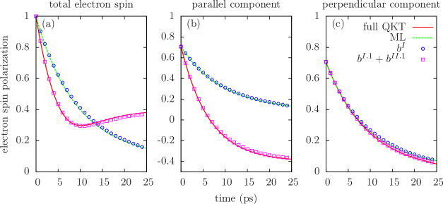
Figure 1: (Color online) Time evolution of the total electron spin polarization (a) and its components parallel (b) and perpendicular (c) to the Mn spin assuming the electrons to be initially spin polarized along a direction at an angle of $45^{\circ}$ relative to the Mn magnetization. The solid red line describes the spin dynamics according to the full quantum kinetic theory, the dashed green line shows its Markov limit (analytic solutions, cf. appendix A). Blue circles and purple squares correspond to approximate quantum kinetic calculations where only a subset of source terms for the correlations (as indicated in the key of the figure) has been accounted for.

The decoupling of the equations of motion in the Markov limit enables us to find analytical solutions for Eq. (10). To this end we split the electron spin into its components parallel and perpendicular to the Mn spin according to:

$$\langle\mathbf{s}_{\mathbf{k}_{1}}\rangle =s^{\|}_{\mathbf{k}_{1}}\frac{\langle\mathbf{S}\rangle}{S}+s^{\perp}_{\mathbf{k}_{1}}\bigg{(}\sin(\omega_{M}t)\frac{\langle\mathbf{S}\rangle\times\langle\mathbf{s}_{\mathbf{k}_{1}}(0)\rangle}{|\langle\mathbf{S}\rangle\times\langle\mathbf{s}_{\mathbf{k}_{1}}(0)\rangle|}$$

$$+\cos(\omega_{M}t)\frac{(\langle\mathbf{S}\rangle\times\langle\mathbf{s}_{\mathbf{k}_{1}}(0)\rangle)\times\langle\mathbf{S}\rangle}{|(\langle\mathbf{S}\rangle\times\langle\mathbf{s}_{\mathbf{k}_{1}}(0)\rangle)\times\langle\mathbf{S}\rangle|}\bigg{)},$$ (13)

where $\omega_{M}$ accounts for the precession of the perpendicular component that results from Eq. (10). With this decomposition, Eq. (10) can be rewritten as:

$$\frac{\partial}{\partial t}s^{\|}_{\mathbf{k}_{1}} =\gamma_{\mathbf{k}_{1}}S(\mathbf{s}^{\|}_{\mathbf{k}_{1}})^{2}+\gamma_{\mathbf{k}_{1}}S\frac{n_{\mathbf{k}_{1}}(2-n_{\mathbf{k}_{1}})}{4}$$

$$-\gamma_{\mathbf{k}_{1}}\big{(}\langle S^{2}\rangle-\langle{S^{\|}}^{2}\rangle\big{)}s^{\|}_{\mathbf{k}_{1}},$$ (14a)

$$\frac{\partial}{\partial t}s_{\mathbf{k}_{1}}^{\perp} =\gamma_{\mathbf{k}_{1}}s^{\|}_{\mathbf{k}_{1}}s^{\perp}_{\mathbf{k}_{1}}S-\frac{1}{2}\gamma_{\mathbf{k}_{1}}\big{(}\langle S^{2}\rangle+\langle{S^{\|}}^{2}\rangle\big{)}s^{\perp}_{\mathbf{k}_{1}},$$ (14b)

with

$$\gamma_{\mathbf{k}_{1}} =\frac{J_{sd}^{2}n_{Mn}}{\hbar^{2}V}\pi\sum_{\mathbf{k}}\delta(\omega_{\mathbf{k}_{1}}-\omega_{\mathbf{k}}),$$ (15a)

$$\omega_{M} =\frac{J_{sd}n_{Mn}}{\hbar}S\bigg{(}1+\frac{1}{2}\frac{J_{sd}}{\hbar V}\sum_{\mathbf{k}}\mathcal{P}\frac{n_{\mathbf{k}}-1}{\omega_{\mathbf{k}_{1}}-\omega_{\mathbf{k}}}\bigg{)},$$ (15b)

and $S=|\langle\mathbf{S}\rangle|$. Eq. (14) is a Riccati differential equation with constant coefficients which can be solved analytically. Its solutions can then be fed back into Eq. (14b) for the perpendicular electron spin. The explicit solutions are listed in appendix A.

It is noteworthy that by a rescaling of the time axis according to $\tau:=\gamma_{\mathbf{k}_{1}}t$ all material parameters can be eliminated from Eqs. (14) for the moduli $s^{\|}_{\mathbf{k}_{1}}$ and $s^{\perp}_{\mathbf{k}_{1}}$. Therefore, with this choice of time units and given initial conditions we obtain the same universal solution for all material parameters. Reinserting the solutions for $s^{\|}_{\mathbf{k}_{1}}$ and $s^{\perp}_{\mathbf{k}_{1}}$ into Eq. (13) and choosing again $1/\gamma_{\mathbf{k}_{1}}$ as the unit of time, we conclude that for given initial conditions the time trace of the electron spin $\langle\mathbf{s}_{\mathbf{k}_{1}}\rangle$ is affected by the material parameters only via the ratio $\omega_{M}/\gamma_{\mathbf{k}_{1}}$.

III Numerical results

The quantum kinetic equations of motion (7) have been solved numerically and compared with their Markov limit (10) for different initial conditions in a three dimensional bulk DMS. The initial electron distribution over the single particle energies $E_{\mathbf{k}}$ is taken to be Gaussian with its center at $E_{k=0}$ and a standard deviation of $\sigma=3\textrm{ meV}$ while the initial magnitude of the Mn spin is set to $\frac{1}{2}\hbar$ (i.e., $20\%$ of its maximal value). The material parameters used were the same as in Ref. Thurn et al., 2013a for Zn_0.93Mn_0.07Se with $J_{sd}=12\textrm{ meVnm}^{3}$ and $m_{e}=0.21m_{0}$.

First, we shall discuss results where at the beginning of the simulation the electron spins are assumed to be totally polarized in a direction with an angle of $45^{\circ}$ with respect to the Mn magnetization vector. Displayed in Fig. 1 is the corresponding time evolution of the electron spin; part (a) shows the total electron spin, while in parts (b) and (c) the components parallel and perpendicular to the Mn magnetization are plotted, respectively. The full quantum kinetic results are plotted as solid red lines whereas curves derived from the analytical solutions of the Markov limit equations are depicted as dashed green lines.

As seen from Fig. 1 (a), the dynamics predicted by the full theory is qualitatively different from the Markovian result. On a short time scale (for our parameters $t<5$ ps), the electron spin decays much faster for the full solution than in the Markov limit. Subsequently, the quantum kinetic curve exhibits a non-monotonic time dependence and the electron spin eventually approaches a finite value. In contrast, in the Markov limit, we find a monotonic, almost exponential decay for all times. From the explicit analytical expression (cf. appendix A) it is seen that the long time limit of the electron spin in the Markov limit is zero.

The origin of the non-monotonic behavior can be understood by splitting the total electron spin into its components parallel [Fig. 1 (b)] and perpendicular [Fig. 1 (c)] to the Mn spin. Both spin components decrease almost exponentially in the ML as well as in the full QKT. The time evolution of the perpendicular spin component essentially yields the same results for the full quantum kinetic calculation and the Markov limit. In the full QKT, however, the parallel spin component changes its sign and converges to a finite negative value, whereas both spin components in the ML and the perpendicular spin component of the QKT drop to zero. When the parallel spin component in the full QKT crosses the zero line, its modulus has a minimum which leads to a minimum in the total spin.

The obvious discrepancy between the different levels of theory with regard to the dynamics of the parallel spin component does not arise due to the assumption of a short memory in the ML. This can be seen from calculations, where only the source terms ${b_{l_{1}n_{1}\mathbf{k}_{1}}^{l_{2}n_{2}\mathbf{k}_{2}}}^{I}$, i.e., the terms used to derive the ML in the first place, have been taken into account but the finite memory expressed by the retardations in Eq. 8 are still kept [blue circles in Fig. 1]. The resulting curves almost coincide with the Markovian calculation. The main difference between the full QKT and the ML is due to the source term ${b_{l_{1}n_{1}\mathbf{k}_{1}}^{l_{2}n_{2}\mathbf{k}_{2}}}^{II.1}$, which is demonstrated by simulations that incorporate only ${b_{l_{1}n_{1}\mathbf{k}_{1}}^{l_{2}n_{2}\mathbf{k}_{2}}}^{I.1}$ and ${b_{l_{1}n_{1}\mathbf{k}_{1}}^{l_{2}n_{2}\mathbf{k}_{2}}}^{II.1}$ [purple squares in Fig. 1]. The results of these calculations agree very well with the predictions of the full theory, suggesting that all other source terms are of minor importance, at least for the parameters used here. It should be noted, that especially the term ${b_{l_{1}n_{1}\mathbf{k}_{1}}^{l_{2}n_{2}\mathbf{k}_{2}}}^{II.1}$, like ${b_{l_{1}n_{1}\mathbf{k}_{1}}^{l_{2}n_{2}\mathbf{k}_{2}}}^{II.2}$ and ${b_{l_{1}n_{1}\mathbf{k}_{1}}^{l_{2}n_{2}\mathbf{k}_{2}}}^{III}$, gives contributions to the reduced electron density matrices in the order of $\mathcal{O}(J_{sd}^{3})$ while the leading order contributions of the correlations are of $\mathcal{O}(J_{sd}^{2})$. Thus, our results imply that a proper description of the coupled electron and Mn spin dynamics requires a treatment beyond perturbation theory.

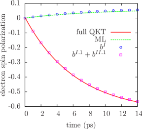
Figure 2: (Color online) Dynamics of the electron spin polarization for initially unpolarized electron spins. Line styles and symbols have the same meaning as in Fig. 1.

The effect of these higher order contributions on the dynamics is particularly dramatic in the case of initially unpolarized electron spins. Corresponding results are displayed in Fig. 2. Here, even the sign of the spin polarization is opposite for the QKT and ML calculations. Furthermore, also the predictions concerning the magnitude of the spin polarization deviate significantly.

IV Interpretation of the source terms

By the numerical analysis in the last section, we were able to trace back the difference between the full quantum kinetic theory and its Markov limit to a few selected source terms for the correlations in Eqs. (7). In this section, we shall give a physical interpretation to the individual source terms which will enable us to understand what determines their relative importance.

First of all, ${b_{l_{1}n_{1}\mathbf{k}_{1}}^{l_{2}n_{2}\mathbf{k}_{2}}}^{I.1}$ is the most important source term, because it starts the correlation dynamics, i.e., without these sources the correlations would stay zero for all times. In the Markov limit, ${b_{l_{1}n_{1}\mathbf{k}_{1}}^{l_{2}n_{2}\mathbf{k}_{2}}}^{I.1}$ yields a Landau-Lifshitz-Gilbert-like damping term described in Eq. (12) and a spin transfer term proportional to the Mn spin $\langle\mathbf{S}\rangle$. ${b_{l_{1}n_{1}\mathbf{k}_{1}}^{l_{2}n_{2}\mathbf{k}_{2}}}^{I.2}$ provides corrections for Pauli blocking to the transfer term and yields another LLG-like damping term, where the electron spin appears twice in the double cross product (cf. Eq. (10)). As seen above, the quantum kinetic ${b_{l_{1}n_{1}\mathbf{k}_{1}}^{l_{2}n_{2}\mathbf{k}_{2}}}^{I}$ contributions act similarly to their Markov limit counterparts. The dominant role of these terms is further emphasized by the fact that they are the leading terms in a perturbative treatment with respect to the exchange coupling constant $J_{sd}$.

In order to understand the meaning of the ${b_{l_{1}n_{1}\mathbf{k}_{1}}^{l_{2}n_{2}\mathbf{k}_{2}}}^{II}$ terms, it is instructive to reformulate the equations of motion of the QKT by introducing new correlation functions according to:

$$Q^{\alpha\mathbf{k}_{2}}_{\beta\mathbf{k}_{1}}:=\sum_{\stackrel{{\scriptstyle l_{1}l_{2}}}{{n_{1}n_{2}}}}S^{\beta}_{n_{1}n_{2}}s^{\alpha}_{l_{1}l_{2}}Q_{l_{1}n_{1}\mathbf{k}_{1}}^{l_{2}n_{2}\mathbf{k}_{2}},$$ (16)

which are summed over the electron band and Mn state indices. Here, we use the conventions $\alpha=0\dots 3$ with $s^{0}_{l_{1}l_{2}}=\delta_{l_{1}l_{2}}$ and $\beta=1\dots 3.$ From Eq. (7c), we obtain the following equations of motion for the summed correlations:

$$\frac{\partial}{\partial t}Q^{0\mathbf{k}_{2}}_{\beta\mathbf{k}_{1}}= -i(\omega_{\mathbf{k}_{2}}-\omega_{\mathbf{k}_{1}})Q^{0\mathbf{k}_{2}}_{\beta\mathbf{k}_{1}}+{b^{0\mathbf{k}_{2}}_{\beta\mathbf{k}_{1}}}^{\textrm{Res}}$$ (17a)

$$\frac{\partial}{\partial t}Q^{{\alpha}\mathbf{k}_{2}}_{\beta\mathbf{k}_{1}}= -i(\omega_{\mathbf{k}_{2}}-\omega_{\mathbf{k}_{1}})Q^{{\alpha}\mathbf{k}_{2}}_{\beta\mathbf{k}_{1}}+{b^{{\alpha}\mathbf{k}_{2}}_{\beta\mathbf{k}_{1}}}^{\textrm{Res}}$$

$$+\sum_{\kappa\lambda}\epsilon_{\alpha\kappa\lambda}\omega_{M}^{\kappa}Q^{\lambda\mathbf{k}_{2}}_{\beta\mathbf{k}_{1}}+\sum_{\kappa\lambda}\epsilon_{\beta\kappa\lambda}\omega_{E}^{\kappa}Q^{\alpha\mathbf{k}_{2}}_{\lambda\mathbf{k}_{1}},$$ (17b)

where

$$\omega^{\alpha}_{M}= \frac{J_{sd}}{\hbar}n_{Mn}\langle S^{\alpha}\rangle,$$ (18a)

$$\omega^{\alpha}_{E}= \frac{J_{sd}}{\hbar}\frac{1}{V}\sum_{\mathbf{k}}\langle s_{\mathbf{k}}^{\alpha}\rangle,$$ (18b)

$${b^{\alpha\mathbf{k}_{2}}_{\beta\mathbf{k}_{1}}}^{\textrm{Res}}= \sum_{\stackrel{{\scriptstyle l_{1}l_{2}}}{{n_{1}n_{2}}}}S^{\beta}_{n_{1}n_{2}}s^{\alpha}_{l_{1}l_{2}}\big{[}{b_{l_{1}n_{1}\mathbf{k}_{1}}^{l_{2}n_{2}\mathbf{k}_{2}}}^{I}+{b_{l_{1}n_{1}\mathbf{k}_{1}}^{l_{2}n_{2}\mathbf{k}_{2}}}^{III}\big{]}$$ (18c)

and $\epsilon_{\alpha\beta\gamma}$ is the Levi-Civita symbol. We note in passing that the residual sources ${b^{\alpha\mathbf{k}_{2}}_{\beta\mathbf{k}_{1}}}^{\textrm{Res}}$ contain a term resulting from ${b_{l_{1}n_{1}\mathbf{k}_{1}}^{l_{2}n_{2}\mathbf{k}_{2}}}^{III.1}$ which cannot be expressed by the summed correlations. Thus, Eqs. (17) are numerically advantageous only if ${b_{l_{1}n_{1}\mathbf{k}_{1}}^{l_{2}n_{2}\mathbf{k}_{2}}}^{III.1}$ is disregarded. The point here is that the two terms in Eq. (17b) originating from ${b_{l_{1}n_{1}\mathbf{k}_{1}}^{l_{2}n_{2}\mathbf{k}_{2}}}^{II.1}$ and ${b_{l_{1}n_{1}\mathbf{k}_{1}}^{l_{2}n_{2}\mathbf{k}_{2}}}^{II.2}$ both involve the Levi-Civita symbol and can therefore be interpreted as describing precessions. This can be made more explicit, e.g., by introducing a vector with components $\alpha$ according to

$$(\mathbf{Q}^{\phantom{\alpha}\mathbf{k}_{2}}_{\beta\mathbf{k}_{1}})_{\alpha}=Q^{\alpha\mathbf{k}_{2}}_{\beta\mathbf{k}_{1}}.$$ (19)

Then, the first of these terms, which stems from ${b_{l_{1}n_{1}\mathbf{k}_{1}}^{l_{2}n_{2}\mathbf{k}_{2}}}^{II.1}$, can be written as a cross product:

$$\bm{\omega}_{M}\times\mathbf{Q}^{\phantom{\alpha}\mathbf{k}_{2}}_{\beta\mathbf{k}_{1}}$$ (20)

indicating a precession of the vector $\mathbf{Q}^{\phantom{\alpha}\mathbf{k}_{2}}_{\beta\mathbf{k}_{1}}$ around the direction $\bm{\omega}_{M}$ of the Mn magnetization with the same frequency as the mean field precession of the electron spin. Likewise, the term originating from ${b_{l_{1}n_{1}\mathbf{k}_{1}}^{l_{2}n_{2}\mathbf{k}_{2}}}^{II.2}$ has a similar structure. It can also be written as a cross product

$$\bm{\omega}_{E}\times\mathbf{Q}^{\alpha\mathbf{k}_{2}}_{{\phantom{\beta}}\mathbf{k}_{1}},$$ (21)

where now the index $\beta$ is associated with the components of a vector $\mathbf{Q}^{\alpha\mathbf{k}_{2}}_{{\phantom{\beta}}\mathbf{k}_{1}}$ formed from the correlations according to

$$(\mathbf{Q}^{\alpha\mathbf{k}_{2}}_{\phantom{\beta}\mathbf{k}_{1}})_{\beta}=Q^{\alpha\mathbf{k}_{2}}_{\beta\mathbf{k}_{1}},$$ (22)

i.e., now we are dealing with a precession around the direction $\bm{\omega}_{E}$ of the electron spin. Thus, not only the average spins of the electrons and Mn atoms exhibit a precession dynamics, but also their correlations, which is represented in the equations of motion by the ${b_{l_{1}n_{1}\mathbf{k}_{1}}^{l_{2}n_{2}\mathbf{k}_{2}}}^{II}$ terms.

Finally, the physical meaning of the ${b_{l_{1}n_{1}\mathbf{k}_{1}}^{l_{2}n_{2}\mathbf{k}_{2}}}^{III}$ source terms becomes clear by noting that their structure is analogous to the structure of the ${b_{l_{1}n_{1}\mathbf{k}_{1}}^{l_{2}n_{2}\mathbf{k}_{2}}}^{I}$ terms, where the products of electron and Mn density matrices are replaced by the corresponding unfactorized correlation functions. Thus, the ${b_{l_{1}n_{1}\mathbf{k}_{1}}^{l_{2}n_{2}\mathbf{k}_{2}}}^{III}$ sources provide the correlated parts of the ${b_{l_{1}n_{1}\mathbf{k}_{1}}^{l_{2}n_{2}\mathbf{k}_{2}}}^{I}$ sources which represented a Landau-Lifshitz-Gilbert-like dynamics including Pauli blocking.

Now that all source terms have been physically interpreted, let us come back to the question of their relative importance in the case considered numerically in subsection III. As already noted, the sources ${b_{l_{1}n_{1}\mathbf{k}_{1}}^{l_{2}n_{2}\mathbf{k}_{2}}}^{I}$ always play a pivotal role, since no correlations would build up without these terms. The importance of the remaining terms depends on the physical situation. Looking at the definition Eq. (7d-f) of the sources, it is seen that the terms ${b_{l_{1}n_{1}\mathbf{k}_{1}}^{l_{2}n_{2}\mathbf{k}_{2}}}^{X.2}$, with $X\in\{I,II,III\}$, comprise similar factors as the corresponding contributions ${b_{l_{1}n_{1}\mathbf{k}_{1}}^{l_{2}n_{2}\mathbf{k}_{2}}}^{X.1}$, except that the former contain an additional factor proportional to the electron density matrix $C_{l_{1}\mathbf{k}_{1}}^{l_{2}}$. From this observation we can conclude that the ${b_{l_{1}n_{1}\mathbf{k}_{1}}^{l_{2}n_{2}\mathbf{k}_{2}}}^{X.2}$ sources should be less important than the ${b_{l_{1}n_{1}\mathbf{k}_{1}}^{l_{2}n_{2}\mathbf{k}_{2}}}^{X.1}$ terms, if the electron density is moderate, as it is the case here. A criterion for being in the low density limit is particularly easy to formulate for the ${b_{l_{1}n_{1}\mathbf{k}_{1}}^{l_{2}n_{2}\mathbf{k}_{2}}}^{II}$ terms, since Eq. (7e) implies that ${b_{l_{1}n_{1}\mathbf{k}_{1}}^{l_{2}n_{2}\mathbf{k}_{2}}}^{II.2}$ is negligible compared with ${b_{l_{1}n_{1}\mathbf{k}_{1}}^{l_{2}n_{2}\mathbf{k}_{2}}}^{II.1}$ if $N_{Mn}\gg N_{e}$ which is fulfilled in our simulations. However, it is more challenging to give a condition for the negligibility of the ${b_{l_{1}n_{1}\mathbf{k}_{1}}^{l_{2}n_{2}\mathbf{k}_{2}}}^{I.2}$ term, as it strongly depends on the electron distribution in k-space.

Finally, since the ${b_{l_{1}n_{1}\mathbf{k}_{1}}^{l_{2}n_{2}\mathbf{k}_{2}}}^{III}$ sources have the same structure as the ${b_{l_{1}n_{1}\mathbf{k}_{1}}^{l_{2}n_{2}\mathbf{k}_{2}}}^{I}$ term, except that the correlations $Q_{l_{1}n_{1}\mathbf{k}_{1}}^{l_{2}n_{2}\mathbf{k}_{2}}$ take the place of the product $C_{l_{1}\mathbf{k}_{1}}^{l_{2}}M_{n_{1}}^{n_{2}}$, they will be of minor importance if the relation $\frac{Q_{l_{1}n_{1}\mathbf{k}_{1}}^{l_{2}n_{2}\mathbf{k}_{2}}}{C_{l_{1}\mathbf{k}_{1}}^{l_{2}}M_{n_{1}}^{n_{2}}}\ll 1$ is satisfied. The latter relation is expected to hold, when the conditions for the applicability of the correlation expansion are fulfilled. The numerical results shown in Fig. 1 indicate that the ${b_{l_{1}n_{1}\mathbf{k}_{1}}^{l_{2}n_{2}\mathbf{k}_{2}}}^{III}$ terms provide insignificant quantitative corrections which confirms the consistency of the correlation expansion approach.

The fact that a source contains correlations is, however, not sufficient for concluding that it can be neglected compared with the ${b_{l_{1}n_{1}\mathbf{k}_{1}}^{l_{2}n_{2}\mathbf{k}_{2}}}^{I}$ terms, which do not involve correlations. In particular, the ${b_{l_{1}n_{1}\mathbf{k}_{1}}^{l_{2}n_{2}\mathbf{k}_{2}}}^{II.1}$ term was shown to qualitatively modify the spin dynamics (cf. Figs. 1 and 2). In view of our interpretation of the ${b_{l_{1}n_{1}\mathbf{k}_{1}}^{l_{2}n_{2}\mathbf{k}_{2}}}^{II.1}$ term, this implies physically that accounting for the precession of the correlations around the Mn magnetization is essential for a correct description of the spin dynamics. This also explains why previous studies in Refs. Thurn et al., 2013a and Thurn et al., 2013b reported a negligible contribution from the ${b_{l_{1}n_{1}\mathbf{k}_{1}}^{l_{2}n_{2}\mathbf{k}_{2}}}^{II.1}$ term, since there a situation was considered, where the average Mn spin was initially set to zero which suppresses the precession.

The features of the spin dynamics predicted in this article manifest themselves in the time evolution of the spin polarization which is a quantity accessible experimentally, e.g., by time- and polarization-resolved photoluminescence or Faraday-/Kerr-rotation measurementsHübner and Oestreich (2008). Favorable for the observation of such effects should be experiments measuring the time dependence of the spin polarization as well as the its equilibrium value where the angle between the Mn magnetization and the initial electron spin polarization induced by a circularly polarized laser beam is varied. For our purposes, bulk materials are preferable compared with, e.g. quantum wells, since for heterostructures, the anisotropy with respect to growth axis as well as structure inversion asymmetry can play a roleBychkov and Rashba (1984) which would make it hard to separate the angular dependence predicted by our theory from anisotropy effects. Furthermore, II-VI DMS should be better suited for the proposed experiment than III-V DMS, since they have the advantage of isoelectrical doping. In III-V materials, the Bir-Aronov-Pikus interactionBir et al. (1975) between electron and hole spins can dominate the spin dynamicsJiang et al. (2009), while for II-VI DMS with sufficiently high Mn doping the s-d-exchange interaction is typically the most important spin relaxation mechanismWu et al. (2010).

V Summary

In this article, we have analyzed the spin dynamics of conduction band electrons in Mn doped bulk DMS induced by the s-d-exchange interaction. In contrast to our previous studies Thurn et al. (2013a, b), we now assume a non-zero Mn magnetization. This naturally leads to a distinction between the electron spin dynamics of the components parallel and perpendicular to the Mn spin which introduces an anisotropy in the spin relaxation. Starting from a microscopic quantum kinetic theory based on correlation expansion we have derived the Markov limit yielding equations similar to the widely used phenomenological Landau-Lifshitz-Gilbert equations. Our derivation yields microscopic expressions for the parameters in the Landau-Lifshitz-Gilbert equations and allows us to identify some quantum corrections. The resulting rate equations were solved analytically.

Numerical simulations within the quantum kinetic theory revealed that, while the dynamics of the perpendicular electron spin component can be well described by the Markovian theory, the parallel component exhibits qualitative deviations between the full quantum kinetic and the corresponding Markovian results. The differences between both levels of theory manifest themselves in a non-monotonic temporal behavior of the total spin in the quantum kinetic theory as opposed to an almost exponential monotonic decay predicted by the Markovian theory. Moreover, for certain excitation conditions, even the sign of the spin polarization differs between these levels of theory.

A detailed analysis allowed us to assign a physical interpretation to all source terms for the correlations and to understand their relative importance found in our numerical studies. With the help of this analysis and our numerical results, the deviations between the full quantum kinetic theory and its Markov limit were traced back to the neglect of a precession dynamics of the correlations in the Markov theory. This precession is missing in the Markov limit not because of the assumption of a short memory but due to the perturbative treatment that is implicit in this approach.

Appendix A Analytical solutions of the Markov equations

Eq. (14a) is a Riccati differential equation

$$\frac{\partial}{\partial t}{s^{\|}_{\mathbf{k}_{1}}}=f{s^{\|}_{\mathbf{k}_{1}}}^{2}-g{s^{\|}_{\mathbf{k}_{1}}}+h,$$ (23)

with $f=\gamma_{\mathbf{k}_{1}}S$, $g=\gamma_{\mathbf{k}_{1}}\big{(}\langle S^{2}\rangle-\langle{S^{\|}}^{2}\rangle\big{)}$ and $h=\gamma_{\mathbf{k}_{1}}S\frac{n_{\mathbf{k}_{1}}(2-n_{\mathbf{k}_{1}})}{4}$. For $f=0$, which is the case if $S=0$, the solution of Eq. (23) is simply:

$${s^{\|}_{\mathbf{k}_{1}}}(t)=\big{(}{s^{\|}_{\mathbf{k}_{1}}}(0)-\frac{h}{g}\big{)}e^{-gt}+\frac{h}{g}.$$ (24)

For $f\neq 0$, the Riccati equation can be rewritten in terms of a linear differential equation with eigenvalues:

$$\lambda_{1/2}=-\underbrace{\frac{g}{2}}_{=:\mu}\pm\underbrace{\sqrt{\frac{g^{2}}{4}-fh}}_{=:\nu}.$$ (25)

The solution of Eq. (23) is then given by:

$${s^{\|}_{\mathbf{k}_{1}}}(t) =\frac{\mu}{f}-\frac{\nu}{f}\textrm{tanh}\left(\frac{\varphi}{2}+\nu t\right)$$ (26a)

where $\varphi$ is determined by the initial value of ${s^{\|}_{\mathbf{k}_{1}}}$.

Eq. (14b) for the perpendicular spin component assumes the form:

$$\frac{\partial}{\partial t}{s^{\perp}_{\mathbf{k}_{1}}} =\big{(}-\xi+f{s^{\|}_{\mathbf{k}_{1}}}\big{)}{s^{\perp}_{\mathbf{k}_{1}}},$$ (27)

where $\xi=\frac{1}{2}\gamma_{\mathbf{k}_{1}}\left(\langle S^{2}\rangle+\langle{S^{\|}}^{2}\rangle\right)$. Eq. (27) is solved by

$${s^{\perp}_{\mathbf{k}_{1}}}(t)={s^{\perp}_{\mathbf{k}_{1}}}(0)e^{-\xi t}\underbrace{e^{f\int\limits_{0}^{t}{s^{\|}_{\mathbf{k}_{1}}}(t^{\prime})dt^{\prime}}}_{=:I}.$$ (28)

For $f=0$, $I=1$ and the perpendicular spin component decreases exponentially. Inserting the solution for the parallel spin compontent from Eq. (26) for non-zero $f$ yields:

$$I =e^{\mu t}\frac{\textrm{cosh}\left(\frac{\varphi}{2}\right)}{\textrm{cosh}\left(\frac{\varphi}{2}+\nu t\right)}$$ (29a)