Improving protein threading accuracy via combining local and global potential using TreeCRF model

Abstract

(Extended Abstract)

1 Motivation

Protein structure prediction remains to be an open problem in bioinformatics [1]. There are two main categories of methods for protein structure prediction: Free Modeling (FM) and Template Based Modeling (TBM). Protein threading, belonging to the category of template based modeling, identifies the most likely fold with the target by making a sequence-structure alignment between target protein and template protein. Though protein threading has been shown to more be successful for protein structure prediction, it performs poorly for remote homology detection.

Protein residue-residue contacts play critical role in maintaining the proteins’ native structures [5]. Contacts potential has been used to help improve both FM and TBM. For FM, the contacts information can help reduce the degrees of freedom in the conformational search space [16][12][14]. And for TBM, it can help select the templates sharing similar contact map with the target protein [11].

Protein threading with contacts potential is NP-hard [8]. Several approximation algorithms have been proposed to tackle this problem. PROSPECT proposed divide-and-conquer algorithm to find suboptimal threading alignment [18]. RAPTOR formulates the threading problem as an Integer Linear Programming (ILP) and then ILP formulation is relaxed to a linear programming (LP) problem, which is solved by the canonical branch-and-bound method [17]. MRFalign formulates the threading problem as a quadratic programming problem and then solve it using Alternate Direction Alternating Direction Method of Multipliers (ADMM) technique [10].

In this paper , we will present our TreeThreader program based on Tree Conditional Random Field (TreeCRF) model. Not only TreeCRF can capture global contact potential, but also the inference in TreeCRF is efficient. In TreeCRF, the contact pairs of the template are selected to construct a nested graph. The special nested structure allows efficient inference to find the optimum threading alignment. From the view of graphical model, TreeCRF makes a compromise between model capacity and model complexity. As shown in Figure 1, the inference in ChainCRF is efficient [7], but it can’ capture global dependence. In contrast, CRF with general graph structure can capture global dependence, but the inference is very hard. The inference in TreeCRF is efficient and it can capture global dependence.

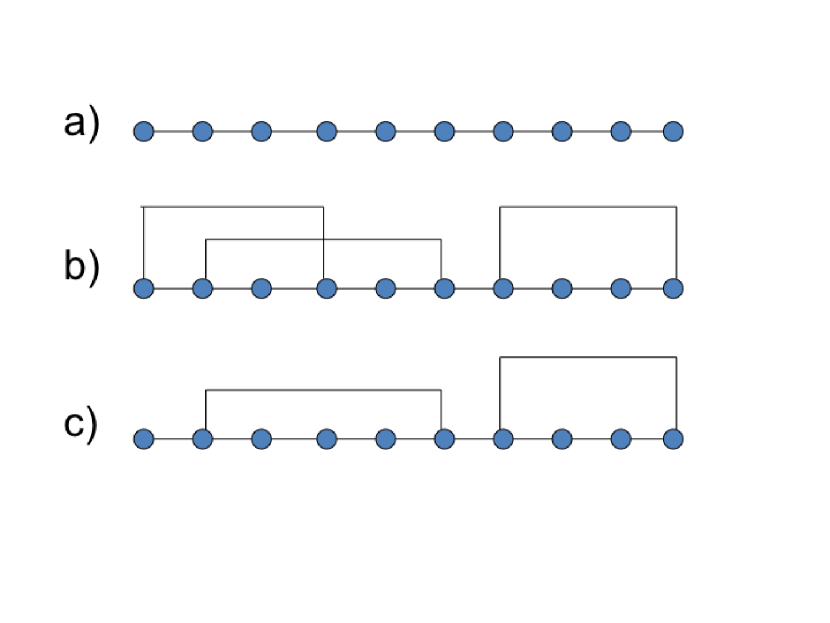
Figure 1: Graphical models with different structures. a) Chain graph: Inference is easy, but it can’t capture global dependence. b) General graph: It can capture global dependence, but inference is hard. c) Nested Graph: Inference is easy and it can capture global dependence.

2 Methods

Given the template protein and the target protein, the framework of our threading method is as follows.

1. Calculate the contact map of the template.

2. Select the most informative contact pairs of the template using dynamic programming.
   

3. Prepare the features used in TreeCRF model.
   

4. Align the target with the template using TreeCRF model.
   

We organize this section as follows. In section 2.1, we will give the dynamic programming algorithm for selecting the most informative contact pairs of the template. Then in section 2.2, we will describe our treeCRF model and the details of the inference algorithm. In section 2.3, we will describe the alignment features used in TreeCRF.

2.1 Select the most informative contact pairs

Given a contact map $G=(V,E)$, we select the most informative contact pairs by solving the following optimization problem.

$$\max_{\begin{subarray}{c}\quad G^{\prime}=(V,E^{\prime})\\ E^{\prime}\subseteq E\\ G^{\prime}\text{ is nested}\end{subarray}}\sum_{(i,j)\in E^{\prime}}C(i,j)$$ (1)

Here, $C(i,j)$ means the contact potential measuring the importance of the contact pair $(i,j)$. Two kinds of contact potential are used in our method: 1) Mutual information (MI) between the sequence profiles of the two residues. 2) Liang-potential [9].

We solve the optimization problem 1 using the following dynamic programming algorithm.

$$M(i,j)=\max\begin{cases}M(i+1,j-1)+C(i,j)\\ M(i,j-1)\\ M(i-1,j)\\ \max_{i<k<j}M(i,k)+M(k+1,j)\end{cases}\textbullet$$ (2)

• Here, $M(i,j)$ denotes the optimum from residue the $i$ to the residue $j$. The optimal nested graph can be constructed by the standard traceback procedure of the dynamic programming algorithm.

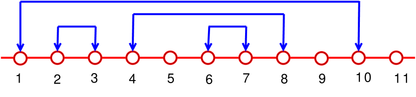
Figure 2: An example of nested graph

Each nested graph can be represented by a serial of nodes with different types ($L$, $R$, $P$ and $B$). Type of the node indicates the direction of the subgraph (left, right, pair and bifurcation). For example, the nested graph in figure 2 can be represented as {$R(1,11)$, $P(1,10)$, $R(2,9)$, $B(2,8)$, $P(2,3)$, $P(4,8)$, $L(5,7)$, $P(6,7)$}.

2.2 TreeCRF model

Let $T$ denote a template protein and $S$ a target protein. Each protein is associated with some protein features, such as sequence profile and secondary structure. Let $A=\{a_{1},a_{2},\cdots,a_{L}\}$ denote an alignment between $T$ and $S$ where $L$ is the alignment length and $a_{i}$ is one of the three possible states $M$ (Match), $I_{s}$ (Insertion), $I_{t}$ (Delete). In TreeCRF, the probability of an alignment $A$ is calculated as follows.

$$P(A|T,S,\theta)=\frac{1}{Z(T,S)}\exp\{\sum_{i=1}^{L}f(a_{i-1},a_{i},T,S)+\sum_{(i,j)\in E^{\prime}}g(a_{i},a_{j},T,S)\}$$ (3)

• , where $f$ and $g$ denote local alignment potentials and global alignment potential respectively. We will give the details of these alignment potential in Section 2.3. In Eq. 3, $Z_{(}S,T)$ denotes the partition function calculated as

$$Z(S,T)=\sum_{\{a_{1},\cdots,a_{L}\}}\frac{1}{Z(T,S)}\exp\{\sum_{i=1}^{L}f(a_{i-1},a_{i},T,S)+\sum_{(i,j)\in E^{\prime}}g(a_{i},a_{j},T,S)\}$$ (4)

•

In ChainCRF or Hidden Markov Model (HMM) [3], Forward algorithm and Backward algorithm are used to calculate the partial alignment probability $P(a_{1},a_{2},\cdots,a_{k}|T,S,\theta)$ and $P(a_{k},a_{k+1},\cdots,a_{L}|T,S,\theta)$ respectively. Viterbi algorithm is used to calculated the optimal alignment by maximizing the alignment probability.

$$\max_{a_{1},a_{2},\cdots,a_{L}}P(a_{1},a_{2},\cdots,a_{L}|S,T,\theta)$$ (5)

• All the above three algorithm are standard dynamic programming algorithms with time complexity $O(m^{2}n^{2})$, where $m$ and $n$ are the length of the template protein and the target protein respectively.

In contrast, we developed Outside algorithm and Inside algorithm to calculate the partial alignment probability and Tree-Viterbi algorithm to calculate the optimal alignment.

Let $O(i,j)$ and $I(i,j)$ denote the partial alignment probability $P(a_{1},a_{2},\dots,a_{i-1},a_{i},a_{j},a_{j+1},\cdots,a_{L}|T,S,\theta)$ and $P(a_{i},a_{i+1},a_{i+2},\cdots,a_{j-2},a_{j-1},a_{j}|T,S,\theta)$ respectively. $O(i,j)$ and $I(i,j)$ are calculated recursively as follows.

$$O(i,j)=\sum_{a_{i-1},a_{j+1}}[\exp(f(a_{i-1},a_{i},T,S)+f(a_{j},a_{j+1},T,S)+g(a_{i},a_{j},T,S))O(i-1,j+1)]$$ (6)

•

$$I(i,j)=\sum_{a_{i+1},a_{j-1}}[\exp(f(a_{i},a_{i+1},T,S)+f(a_{j-1},a_{j},T,S)+g(a_{i},a_{j},T,S))I(i+1,j-1)]$$ (7)

•

Figure 3 shows the process of the Inside algorithm. The Inside algorithm calculates the partial alignment from the inside to the outside following the tree structure.

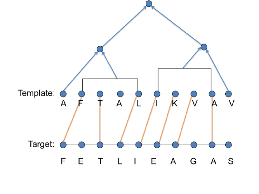
Figure 3: The process of calculating partial alignment probability using Inside algorithm.

ChainCRF	TreeCRF	CRF with general structure
Forward algorithm ($O(mn)$)	Inside algorithm ($O(Kmn)$)	NP-hard
Backward algorithm ($O(mn)$)	Outside algorithm ($O(Kmn)$)	NP-hard
Viterbi algorithm ($O(mn)$)	Tree-Viterbi algorithm ($O(Kmn)$)	NP-hard

Table 1: The comparison between the complexity of ChainCRF, TreeCRF and CRF with general structure

The time complexity of Outside algorithm, Inside algorithm and Tree-Viterbi algorithm is $O(Kmn)$, where $K$ is the number of the selected contact pairs of the template. As shown in Table 1, TreeCRF makes a compromise between model capacity and model complexity.

2.3 Alignment features

The features used to estimate the alignment probability of two residues is as follows.

1. Sequence profile similarity: the profile similarity between two positions is calculated as [15]

   $$S_{aa}(q_{i},p_{j})=\log(\sum_{a=1}^{20}\frac{q_{i}(a)p_{j}(a)}{f(a)})$$ (8)

   • Here, $q_{i}(a)$ and $p_{j}(a)$ denote the frequency of amino acid $a$ at the $i$th position of the template and the $i$th position of the target. And $f(a)$ means the background frequency of amino acid $a$.

2. Secondary structure score: we generate 8-class secondary structure types for the template using DSSP [6] and predict the 3-class secondary structure types for the target using PSIPRED [13]. The secondary structure score is calculated as

   $$SS(\delta;\rho,c)=\log\frac{P(\delta;\rho,c)}{P(\delta)P(\rho,c)}$$ (9)

   Here, $\delta$ the secondary structure type of the template and $(\rho,c)$ means the secondary structure of the target predicted as $\rho$ with confidence $c$.

3. Solvent accessibility (SA) score: Real value SA of the query is predicted by Real-SPINE [2] and SA of template are calculated by DSSP. The SA score is calculated as: $1-2|sa(i)-sa(j)|$ where $sa(i)$ is the residue solvent accessibility of target sequence predicted by Real-Spine and $sa(j)$ is the residue solvent accessibility of the template calculated by DSSP.

4. Dihedral torsion angles: The real value torsion angle of the query is predicted by Real-SPINE and that of template is calculated by DSSP. The difference between predicted angles $(\psi(i)$ and $\phi(i))$ of the query and actual angles $(\psi(j)$ and $\phi(j))$ of the template is characterized

   $$\bigtriangleup=\sqrt{\frac{1}{2}[(\psi(i)-\psi(j))^{2}+(\phi(i)-\phi(j))^{2}]}$$ (10)

5. Environment fitness score: This score measures how well one sequence residue aligns to a specific template environment.

2.4 Results

We constructed PDB25 dataset using PDB-SELECT [4]. Any two proteins in PDB25 share $<25\%$ sequence identity. Then we randomly select 300 protein pairs as training data and another 300 pairs as testing data. There is no redundancy between the training and testing data . The reference structure alignments for the training and testing data are built using TMalign [19].

We compare our TreeCRF threading method, named TreeThreader with the widely used software HHpred [15]. As shown in 2, TreeThreader achieves better performance than HHpred.

	TM-align	HHpred-mac	Tree-Viterbi	Tree-mac
GDT	51.1	33.1	33.9	35.8

Table 2: Reference-dependent alignment accuracy of TreeCRF and HHpred on test dataset of 300 pairs

3 Conclusion

We developed a novel protein threading tool named TreeThreader. Firstly, both local potential and global potential are used in TreeThreader. Secondly, the TheeThreader is very efficient and practical. Results show that TreeThreader achieves better performance than the widely used protein alignment tool HHpred.

References

- [1] Ken A Dill and Justin L MacCallum. The protein-folding problem, 50 years on. Science, 338(6110):1042–1046, 2012.
- [2] Ofer Dor and Yaoqi Zhou. Real-spine: An integrated system of neural networks for real-value prediction of protein structural properties. PROTEINS: Structure, Function, and Bioinformatics, 68(1):76–81, 2007.
- [3] Sean R Eddy. Hidden markov models. Current opinion in structural biology, 6(3):361–365, 1996.
- [4] Sven Griep and Uwe Hobohm. Pdbselect 1992–2009 and pdbfilter-select. Nucleic acids research, page gkp786, 2009.
- [5] M Michael Gromiha and S Selvaraj. Inter-residue interactions in protein folding and stability. Progress in biophysics and molecular biology, 86(2):235–277, 2004.
- [6] Robbie P Joosten, Tim AH Te Beek, Elmar Krieger, Maarten L Hekkelman, Rob WW Hooft, Reinhard Schneider, Chris Sander, and Gert Vriend. A series of pdb related databases for everyday needs. Nucleic acids research, 39(suppl 1):D411–D419, 2011.
- [7] John Lafferty, Andrew McCallum, and Fernando CN Pereira. Conditional random fields: Probabilistic models for segmenting and labeling sequence data. 2001.
- [8] Richard H Lathrop. The protein threading problem with sequence amino acid interaction preferences is np-complete. Protein engineering, 7(9):1059–1068, 1994.
- [9] Xiang Li, Changyu Hu, and Jie Liang. Simplicial edge representation of protein structures and alpha contact potential with confidence measure. Proteins: Structure, Function, and Bioinformatics, 53(4):792–805, 2003.
- [10] Jianzhu Ma, Sheng Wang, Zhiyong Wang, and Jinbo Xu. MRFalign: protein homology detection through alignment of markov random fields. PLoS computational biology, 10(3):e1003500, 2014.
- [11] Jianzhu Ma, Sheng Wang, Zhiyong Wang, and Jinbo Xu. Protein contact prediction by integrating joint evolutionary coupling analysis and supervised learning. In Research in Computational Molecular Biology, pages 218–221. Springer, 2015.
- [12] Debora S Marks, Thomas A Hopf, and Chris Sander. Protein structure prediction from sequence variation. Nature biotechnology, 30(11):1072–1080, 2012.
- [13] Liam J McGuffin, Kevin Bryson, and David T Jones. The psipred protein structure prediction server. Bioinformatics, 16(4):404–405, 2000.
- [14] Mirco Michel, Sikander Hayat, Marcin J Skwark, Chris Sander, Debora S Marks, and Arne Elofsson. Pconsfold: improved contact predictions improve protein models. Bioinformatics, 30(17):i482–i488, 2014.
- [15] Johannes Söding. Protein homology detection by hmm–hmm comparison. Bioinformatics, 21(7):951–960, 2005.
- [16] Sitao Wu, Andras Szilagyi, and Yang Zhang. Improving protein structure prediction using multiple sequence-based contact predictions. Structure, 19(8):1182–1191, 2011.
- [17] Jinbo Xu, Ming Li, Dongsup Kim, and Ying Xu. Raptor: optimal protein threading by linear programming. Journal of bioinformatics and computational biology, 1(01):95–117, 2003.
- [18] Ying Xu and Dong Xu. Protein threading using prospect: design and evaluation. Proteins: Structure, Function, and Bioinformatics, 40(3):343–354, 2000.
- [19] Yang Zhang and Jeffrey Skolnick. Tm-align: a protein structure alignment algorithm based on the tm-score. Nucleic acids research, 33(7):2302–2309, 2005.